Scalar-field quintessence by cosmic shear:
CFHT data analysis and forecasts for DUNE

Abstract

A light scalar field, minimally or not-minimally coupled to the metric field, is a well-defined candidate for the dark energy, overcoming the coincidence problem intrinsic to the cosmological constant and avoiding the difficulties of parameterizations. We present a general description of the weak gravitational lensing valid for every metric theory of gravity, including vector and tensor perturbations for a non-flat spatial metric. Based on this description, we investigate two minimally-coupled scalar field quintessence models using VIRMOS-Descart and CFHTLS cosmic shear data, and forecast the constraints for the proposed space-borne wide-field imager DUNE.

1 Introduction

There is an overwhelming evidence that the description of the observed universe cannot rely only on the assumption of the Copernican principle, on the general relativity, and on the Standard Model of particle physics, eventually extended to include a dark matter candidate [1]. We shall define dark energy as anything which represents the failure of some of these assumptions: i) It could be a signature of the dynamical effect of inhomogeneities, not properly averaged when accounting for the background dynamics [2]. ii) Gravitational interactions (on cosmological scales) could be not described by the Hilbert-Einstein action, requiring e.g. the inclusion of higher-order terms as in scalar-tensor theories of gravity [3] or a formulation in more than four dimensions, as in braneworld scenarios or superstring theories [4]. iii) Dark energy is an effective “matter” field, often dubbed quintessence [5], not clustering on the observed scales and possibly coupled to the matter fields [6], provided the weak equivalence principle is preserved. A combination of these options is the last possibility, like in extended quintessence scenarios [7]. One can therefore define classes of models, characterized by definite observational and experimental signatures [8].

The weak gravitational lensing by large scale structures, or cosmic shear, is a geometrical observable which depends on both background evolution and structures formation [9]. Therefore it is a promising tool to investigate dark energy , allowing one to explore in unbiased way the low-redshift universe where dark energy mostly acts [10, 11]. Cosmic shear has been exploited to investigate ordinary quintessence scenarios, considering a parametrization of the quintessence equation of state [10, 11, 12]. We move towards “physics”-inspired models, for the first time using real data along this strategy [13]. This requires a general formulation of weak-lensing, which we achieve just supposing that gravitation is described by a metric theory [14].

2 Geometry of null congruences: cosmic shear

Every galaxy defines a light bundle, or congruence of null geodesics $x^{\mu}(\lambda)=\bar{x}^{\mu}(\lambda)+\xi^{\mu}(\lambda)$ deviating from a fiducial, arbitrary geodesic $\bar{x}^{\mu}$ by a displacement $\xi^{\mu}$, converging at the observer position $O$ (where $\xi^{\mu}=0$), and whose tangent vectors $k^{\mu}\equiv dx^{\mu}/d\lambda$ are solution of $k_{\mu}k^{\mu}=0$ and $k^{\nu}\nabla_{\nu}k^{\mu}=0$ (we take the affine parameter $\lambda$ vanishing in $O$ and increasing toward the past). The shape of the light bundle is described by a deformation tensor $\mathcal{D}^{a}_{\;b}$, whose evolution along the fiducial geodesic (defined by $\bar{k}^{\mu}$) is deduced from the geodesic deviation equation for $\xi^{\mu}$. On the plane $\{n_{1}^{\mu},n_{2}^{\mu}\}$ orthogonal to the line-of-sight ($n^{a}_{\mu}n_{b}^{\mu}=\delta^{a}_{\;b},n^{a}_{\mu}\bar{k}^{\mu}=0$), and setting $\xi_{a}(\lambda)=n^{a}_{\mu}\xi^{\mu}(\lambda)\equiv\mathcal{D}^{b}_{\;a}(\lambda)\dot{\xi}_{b}(0)$, it turns out

$$\ddot{\mathcal{D}}^{a}_{\;b}=\mathcal{R}^{a}_{\;c}\mathcal{D}^{c}_{\;b}$$ (1)

with initial conditions $\mathcal{D}^{a}_{\;b}(0)=0,\dot{\mathcal{D}}^{a}_{\;b}(0)=\delta^{a}_{\;b}$, the dot referring to a derivation with respect to $\lambda$. Here $\mathcal{R}^{a}_{\;b}\equiv R^{\alpha}_{\;\mu\nu\beta}\bar{k}^{\mu}\bar{k}^{\nu}n_{a}^{\alpha}n_{b}^{\beta}=-\frac{1}{2}R_{\mu\nu}\bar{k}^{\mu}\bar{k}^{\nu}\delta^{a}_{\;b}+C^{\alpha}_{\;\;\mu\nu\beta}\bar{k}^{\mu}\bar{k}^{\nu}n_{\alpha}^{a}n_{b}^{\beta}$ is the optical tidal matrix written in terms of the Riemann tensor $R^{\alpha}_{\;\mu\nu\beta}$ or in terms of the Ricci and Weyl tensors, respectively $R_{\mu\nu}$ and $C^{\alpha}_{\;\mu\nu\beta}$. This latter expression highlights the sources of the isotropic and anisotropic deformation of the original image.

In a perturbed universe with metric $g_{\mu\nu}=a^{2}(\eta)(\bar{g}^{\mathrm{RW}}_{\mu\nu}+h_{\mu\nu})$, Equation (1) is solved order-by-order in $h_{\mu\nu}$. Here we consider scalar, vector, and tensor perturbations of the Robertson-Walker metric allowing for curvature,

$$\qquad g_{\mu\nu}\rmd x^{\mu}\rmd x^{\nu}=a^{2}(\eta)\{-(1-2\phi)\rmd\eta^{2}+2B_{i}\rmd\eta\rmd x^{i}+[(1+2\psi)\gamma_{ij}+2E_{ij}]\rmd x^{i}\rmd x^{j}\},$$ (2)

with $\nabla^{i}B_{i}=\nabla^{i}E_{ij}=E^{i}_{i}=0$. The spatial metric $\gamma_{ij}\rmd x^{i}\rmd x^{j}=\rmd\chi^{2}+S_{K}^{2}(\chi)\rmd\Omega^{2}$ is written in terms of the angular diameter distance $S_{K}(\chi)=\sin(\sqrt{K}\chi)/\sqrt{K}$, $K=\{-1,0,1\}$, of the comoving radial distance $\chi$, and of the infinitesimal solid angle $\rmd\Omega^{2}$. Exploiting the conformal invariance of null geodesics, for $\bar{g}_{\mu\nu}=a^{-2}(\eta)g_{\mu\nu}$ the optical tidal matrix reads

$$\qquad\mathcal{R}^{a(0)}_{\;b}=-K\delta^{a}_{\;b}\;,\quad\mathcal{R}^{a(1)}_{\;b}=D^{a}D_{b}(\phi+\psi+B_{\hat{\chi}}+E_{{\hat{\chi}}{\hat{\chi}}})+K(E^{a}_{\;b}-E_{{\hat{\chi}}{\hat{\chi}}}\delta^{a}_{\;b}),$$ (3)

$D_{a}$ being the covariant derivative with respect to the spatial metric $\gamma_{ij}$ and ${\hat{\chi}}$ denoting the component along the line-of-sight. Accordingly, Equation (1) leads to

$$\ddot{\mathcal{D}}^{(0)}=-K\mathcal{D}^{(0)}\;,\quad\ddot{\mathcal{D}}^{(1)}=-K\mathcal{D}^{(1)}+\mathcal{R}^{(1)}\mathcal{D}^{(0)}.$$ (4)

The solution $\mathcal{D}=\mathcal{D}^{(0)}+\mathcal{D}^{(1)}$ is finally rescaled by the (angular) distance of the source galaxy, $d_{\mathrm{A}}(\lambda)$, to get the amplification matrix $\mathcal{A}_{ab}=\mathcal{D}_{ab}(\lambda)/d_{\mathrm{A}}(\lambda)$; its diagonal and off-diagonal terms, which account for the isotropic and anisotropic deformation of the original image, are the observed quantities. Eventually, one has to integrate over the distribution of sources $n(\chi)$ along the line-of-sight (notice that $\rmd\lambda=a^{2}\rmd\chi$). Usually a fitting function of the form $n(z)\propto(z/z_{\mathrm{s}})^{\alpha}\exp[-(z/z_{\mathrm{s}})^{\beta}]$ is taken to reproduce the observed distribution of sources as a function of redshift $z$. Neglecting vector and tensor perturbations, from $\mathcal{R}^{a(1)}_{\;b}\equiv D^{a}D_{b}\Phi$ the convergence field $\kappa=(1-\Tr\mathcal{A})$ reads

$$\kappa(\boldsymbol{\theta})=\int_{0}^{z_{H}}\rmd z\,n(z)\kappa(\boldsymbol{\theta},z)=\int_{0}^{\chi_{H}}\rmd\chi\,n(\chi)\int_{0}^{\chi}\rmd\chi^{\prime}\,\frac{S_{K}(\chi)S_{K}(\chi^{\prime}-\chi)}{S_{K}(\chi^{\prime})}\Delta_{2}\Phi[S_{K}(\chi^{\prime})\boldsymbol{\theta},\chi^{\prime}]\\$$ (5)

where the deflecting potential $\Phi$ is calculated solving the field (e.g. Einstein) equations.

In the flat sky approximation, the convergence and shear power spectra are

$$P_{\kappa}(\ell)=P_{\gamma}(\ell)=\frac{1}{4}\int\rmd\chi\,g^{2}(\chi)\left[k^{4}P_{\Phi}(k,\chi)\right]_{k=\ell/S_{K}(\chi)}$$ (6)

where $g(\chi)=\int_{\chi}^{\chi_{\mathrm{H}}}\rmd\chi^{\prime}\,n(\chi^{\prime})S_{K}(\chi^{\prime}-\chi)/S_{K}(\chi^{\prime})$ and $P_{\Phi}$ is the three-dimensional power spectrum of the deflecting potential. Two-point correlation functions in the real space, like top-hat shear or aperture mass variances, are filtered integrals of this quantity [9].

3 Quintessence by cosmic shear: Parameterizations vs “physical” models

The use of parameterizations for the quintessence equation of state generally assumes a Friedmann-Robertson-Walker universe, thus excluding a priori other options for the dark energy sector. Moreover, every parametrization is affected by the choice of a dataset-dependent pivot redshift [10], by the consistency with a model for the speed of sound determining the formation of structure, and by the large number of parameters required to suitably account for a “realistic” dynamics over a wide range of redshift [15]. Dealing with “physics”-inspired models one would overcome these problems, aiming to investigate if a class of theory is compatible with observations at low and high redshift.

We explore two ordinary quintessence scenarios, realized by a self-interacting scalar degree of freedom $Q$ with Ratra-Peebles (RP) and supergravity (SUGRA) potentials

$$V_{\mathrm{RP}}(Q)=M^{4+\alpha}/Q^{\alpha};\quad V_{\mathrm{SUGRA}}(Q)=M^{4+\alpha}\exp(Q^{2}/2M_{\mathrm{Pl}}^{2})/Q^{\alpha}$$ (7)

which guarantee the (partial) solution of the coincidence problem [7]. The mass scale $M$ is uniquely determined once $\alpha$ and the density parameter $\Omega_{\mathrm{Q}}$ are fixed.

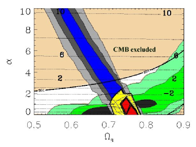
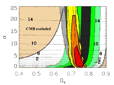
Figure 1: Likelihood analysis of the quintessence parameter space for RP (left) and SUGRA (right) models, marginalizing over $(n_{s},z_{s})$, using CFHT cosmic-shear data (blue contours, at 68, 95, and 99%), the “goldset” of SnIa (green), and both jointly (red). The shaded region is excluded since it corresponds to a location of the first peak of CMB $C_{\ell}^{\mathrm{TT}}$ not compatible with WMAP-3yr data (considering the very conservative range $201\lesssim\ell_{1\mathrm{st}}\lesssim 240$). Dotted lines refer to $\log_{10}M/$GeV; see Equation (7).

Background and perturbations evolution in linear regime are computed solving the Einstein and Klein-Gordon equations by means of a Boltzmann code described in [16]. Dealing with general relativity, on sub-horizon scales one can safely use the Poisson equation to relate the deflecting potential $P_{\Phi}=4P_{\phi}$ to the power spectrum of matter perturbations. In order to account for the non-linear matter power spectrum, we use two linear-to-non-linear mappings [17] (see [14] a generalization in scalar-tensor theories). Although calibrated on $\Lambda$CDM $N$-body simulations, they provide a quite safe recipe also for QCDM models, provided the linear regime is properly taken into account using the correct linear growth factor and the spectra normalized to high-redshift (by CMB). Indeed, the $Q$-field mostly acts on the background dynamics affecting the onset of the non-linear regime, while the successive evolution on small scales (affecting the structure of single galaxies/halos, bias, etc.) is essentially dictated by astrophysical processes.

4 Joint cosmic-shear–SnIa data analysis

We combined VIRMOS-Descart, CFHTLS-deep, and CFHTLS-wide/22 deg² top-hat shear variance data (see [13] for references) to investigate the sensitivity to the description of the non-linear regime [17]. The results look different when using the Peacock & Dodds (1996) or the Smith et al(2003) prescriptions, which are based on different modeling of the non-linear clustering. Notice that both mappings do not include the effects of baryons, not negligible on the scales of interest to cosmic shear [18]. Interestingly, the quintessence parameter space $(\Omega_{\mathrm{Q}},\alpha)$ seems not to be sensitive to non-linear gravitational clustering, probing that quintessence primarily acts on geometry.

Combining the cosmic-shear data with the “goldset” of supernovae Ia (SnIa) [20], figure 1, one can safely constraint RP models ($\alpha<1,\Omega_{\mathrm{Q}}=0.75^{+0.03}_{-0.04}$ at 95%) because of the strong degeneracy between the two observables. More care is needed for SUGRA models, where the superposition of likelihood contours is severely dependent on reliability of their location, ultimately dependent on systematics. Eventually, one can extract the value of the mass scale $M$, whose contours follow the estimate $\log_{10}(M/\mbox{GeV})\simeq(19\alpha-47+\log\Omega_{\mathrm{Q}})/(\alpha+4)$ which holds as long as $Q\sim M_{\mathrm{Pl}}$. Actually, notice that redshift and shear calibration of datasets are a crucial point [19].

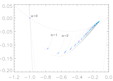
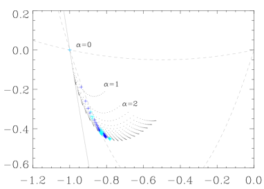
Figure 2: Likelihood analysis of the quintessence parameter space $(\Omega_{\mathrm{Q}},\alpha)$ transposed in the $(w,w^{\prime})$ parameter space (at $z=0$), for RP (left) and SUGRA (right) models, using only the combined cosmic shear data sets. Dark and light crosses refer to points lying respectively within the 68 and 95% confidence levels of the original likelihood, while dots correspond to remaining points of the $(\Omega_{\mathrm{Q}},\alpha)$ grid. Solid and dashed lines correspond to the $c^{2}_{\mathrm{s}}<1$ constraint for the $Q$-field and the class of “freezing” quintessence model, respectively. The cosmological constant is recovered for $\alpha=0$.

Exploiting the one-to-one relation between $(\Omega_{\mathrm{Q}},\alpha)$ and the values of the quintessence equation of state and its time derivatives (valid for $\alpha\neq 0$) at whatever redshift, we translate the likelihood contours of the joint analysis in a $(w,w^{\prime})$ parameter space ($w^{\prime}\equiv\rmd w/\rmd\ln a$), evaluated at $z=0$; see figure 2. This is useful to compare the models at hand with other classes of models [21], and with the dynamical constraints $w^{\prime}>-3(1-w^{2})$ (solid line), corresponding to a $Q$-field’s speed of sound $c^{2}_{\mathrm{s}}<1$, and $3w(1+w)<w^{\prime}<0.2w(1+w)$ (dashed line), characterizing the so-called “freezing” models. For every set of points characterized by the same $\alpha$ (linearly varying by $\Delta\alpha=1$), points span the $\Omega_{\mathrm{Q}}$ range $[0.4,0.9]$ from top to bottom (linear steps $\Delta\Omega_{\mathrm{Q}}=0.025$).

5 Wide surveys: forecasts

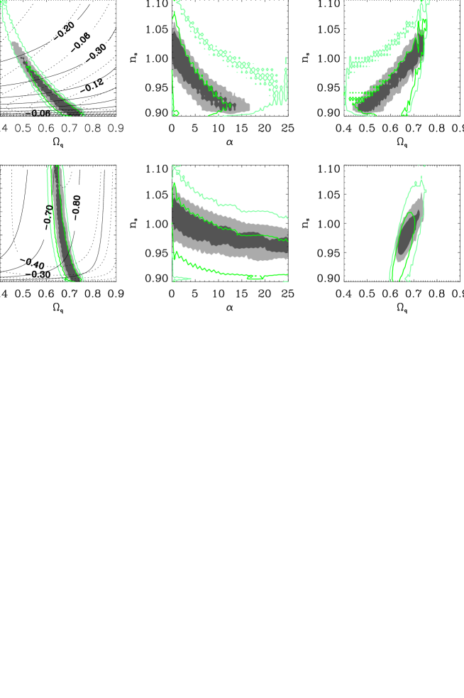
Figure 3: Likelihood analysis of the top-hat shear variance based on a synthetic realization of the full 170 deg² CFHTLS-wide survey (filled contours; 68 and 95% c.l.) and considering only scales $\gtrsim 20$ arcmin (empty contours), for RP (upper) and SUGRA (lower). Solid (dotted) lines in the $(\Omega_{q},\alpha)$ plane represent the value of $w$ ($w^{\prime}$) at $z=0$.

Focusing on wide surveys (figure 3), one can investigate angular scales where the contamination of the non-linear regime is reduced (a residual being always present because of the integration along the line-of-sight; see Equation (5)). Using a synthetic realization of the CFHTLS-wide full survey, we performed a likelihood analysis using only angular scales $\gtrsim 20$ arcmin. Since it corresponds to cutting off larger wavemodes $k$, the contours concerning all the cosmological parameters we considered broaden. However, the contours of the quintessence parameter space are less affected by this cut. In particular, SUGRA models seem to be very slightly dependent on $\alpha$ but highly sensitive on $\Omega_{Q}$. Finally, remark that the results depend on $n(z)$, which we suppose to be the same of that measured for the 22 deg² dataset.

This analysis points towards the gain achievable by a very-wide survey, for which the quality image requirements very likely need space-based observations. We thus forecast the improvement on the RP and SUGRA models considering a DUNE-like mission [22], a shallow survey covering $20\,000$ deg². The results depicted in figure 4 illustrate the gain with respect to the full CFHTLS-wide survey. It has to be stressed, however, that this estimation is based on an approximate distribution of sources, assumes a perfect correction of the point spread function, and finally is marginalized over a small number of cosmological parameters.

6 Concluding remarks

Using a general formulation of weak-lensing valid for every metric theory of gravity, we dispose of tools to study several classes of the dark energy sector at both low and high redshift, avoiding the use of parameterizations which difficult a safe combination of data sets and can hardly match any well-defined theory. We investigate two classes of ordinary quintessence models by means of real cosmic shear data, and combining with supernovae data, putting forward the interest of using CMB data to normalize the spectra and thus define the onset of the non-linear regime of structures formation. The contamination of non-linear gravitational clustering can be reduced when disposing of wide surveys, which reasonably require space-based missions to achieve a high-precision characterization of the dark-energy sector.

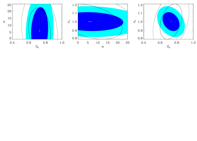
Figure 4: Fisher analysis forecast for a CFHTLS-wide 170 deg² survey (wide/blue ellipses) and a DUNE-like $20\,000$ deg² survey (small/red ellipses; contours at 1 and $2\sigma$) for the $(\Omega_{\mathrm{Q}},\alpha,n_{\mathrm{s}})$ parameter space, marginalizing over $(\tau_{\mathrm{reion}},z_{\mathrm{s}})$. Filled (empty) contours refer to SUGRA (RP) models (for RP, only CFHTLS-wide contours are shown), both centered at the same fiducial model.

References

References

- [1] Peebles P J E and Ratra B 2003, Rev. Mod. Phys. 75 559
- [2] Ellis G F R and Buchert T 2005, Phys. Lett. A 347 38; Kolb E W, Matarrese S and Riotto A 2005, accepted for publication in New Journal of Physics (Preprint: astro-ph/0506534)
- [3] Damour T and Esposito-Farèse G 1992, Class. Quantum Grav.9 2093
- [4] Brax P and van de Bruck C 2003, Class. Quantum Grav.20 R201; Lidsey J E, Wands D and Copeland E J 2000, Phys. Rept. 337 343
- [5] For a review, see Copeland E J, Sami M and Tsujikawa S 2006 (Preprint: hep-th/0603057)
- [6] Amendola L 2000, Phys. Rev. D 62 043511
- [7] Uzan J P 1999, Phys. Rev. D 59 123510; Chiba T 1999, Phys. Rev. D, 60 083508
- [8] Uzan J-P 2006 (Preprint: astro-ph/0605313)
- [9] Mellier Y 1999, ARA&A 37 127; Bartelmann M and Schneider P 2001, Phys. Rept. 340 291
- [10] Hu W and Jain B 2004, Phys. Rev. D 70 043009
- [11] Benabed K and van Waerbeke L 2004, Phys. Rev. D 70 123515
- [12] Jarvis M et al2006, Ap. J. 664 71; Semboloni E et al2006, A&A 452 51; Hoekstra H et al2006, Ap.J. 647 116
- [13] Schimd C, Tereno I, Uzan J-P, Mellier Y et al2006, A&A in press (Preprint: astro-ph/0603158)
- [14] Schimd C, Uzan J-P and Riazuelo A 2005, Phys. Rev. D 71 083512
- [15] Corasaniti P S and Copeland E J 2003, Phys. Rev. D 67 063521
- [16] Riazuelo A and Uzan J-P 2002, Phys. Rev. D 66 023525
- [17] Peacock J A and Dodds S J 1996, MNRAS 280 L19; Smith R E et al2003, MNRAS 341 1311
- [18] White M 2005, Astropart. Phys. 24 334; Zhan H and Knox L 2004, Ap.J. 616 L75
- [19] van Waerbeke L et al2006 (Preprint: astro-ph/0603696)
- [20] Tonry et al2003, Ap.J. 594 1.
- [21] Barger V et al2006, Phys. Lett. B 635 61; Scherrer R J 2006, Phys. Rev. D 73 043502
- [22] Réfrégier A et al2006, Proceedings of SPIE vol 6265 (Preprint: astro-ph/0610062)