The Stellar Populations of M33’s Outer Regions III: Star Formation History

Abstract

We present a detailed analysis of the star formation history (SFH) of three fields in M33 located $\sim 4-6$ visual scale lengths from its nucleus. These fields were imaged with the Advanced Camera for Surveys on the Hubble Space Telescope and reach $\sim 2.5$ magnitudes below the red clump of core helium burning stars. The observed color-magnitude diagrams are modeled as linear combinations of individual synthetic populations with different ages and metallicities. To gain a better understanding of the systematic errors we have conducted the analysis with two different sets of stellar evolutionary tracks which we designate as Padova (Girardi et al. 2000) and Teramo (Pietrinferni et al. 2004). The precise details of the results depend on which tracks are used but we can make several conclusions that are fairly robust despite the differences. Both sets of tracks predict the mean age to increase and the mean metallicity to decrease with radius. Allowing age and metallicity to be free parameters and assuming star formation began $\sim 14$ Gyr ago, we find that the mean age of all stars and stellar remnants increases from $\sim 6$ Gyr to $\sim 8$ Gyr and the mean global metallicity decreases from $\sim-0.7$ to $\sim-0.9$. The fraction of stars formed by 4.5 Gyr ago increases from $\sim 65\%$ to $\sim 80\%$. The mean star formation rate $80-800$ Myr ago decreases from $\sim 30\%$ of the lifetime average to just $\sim 5\%$. The random errors on these estimates are $\sim 10\%$, 1.0 Gyr, and 0.1 dex. By comparing the results of the two sets of stellar tracks for the real data and for test populations with known SFH we have estimated the systematic errors to be $15\%$, 1.0 Gyr, and 0.2 dex. These do not include uncertainties in the bolometric corrections or variations in $\alpha$-element abundance which deserve future study.

1. Introduction

The stellar populations of a galaxy are a fossil record of its formation and evolution and the various physical processes involved. Since the work of Eggen et al. (1962), the ages, kinematics, and chemical compositions of stellar populations in the Galaxy have proved crucial to our understanding of its evolution (see Freeman & Bland-Hawthorne 2002 for a recent review). By the same token, such vital statistics are reshaping our view of nearby galaxies especially those in the Local Group (LG; e.g., Sarajedini et al. 2000; Harbeck et al. 2001; Ferguson et al. 2002; Brown et al. 2003; Lanfranchi & Matteucci 2004; Cole et al. 2005).

A critical tool in this advancement is the stellar color-magnitude diagram (CMD). By comparing the observed distribution of stars in a CMD with the predictions of stellar evolutionary theory one can estimate their ages and metallicities. For star clusters, such a comparison is straightforward relative to the more complex task of disentangling the ages and metallicities of stars in the general field. Nevertheless, the study of field populations has progressed tremendously due in part to advances in CMD analysis techniques and, in particular, the technique of synthetic CMD fitting. Central to this technique is the use of theoretical stellar evolutionary tracks with which one can generate a model CMD for any arbitrary star formation history (SFH). The model CMD can then be compared to the observed CMD to see how closely they match and, thus, how closely the model SFH matches the true SFH.

Various forms of this technique have been applied to galaxies throughout the LG revealing a variety of SFHs (e.g., Tosi et al. 1991; Bertelli et al. 1992; Aparicio et al. 1997; Dohm-Palmer et al. 1997; Tolstoy et al. 1998; Gallart et al. 1999; Hernandez et al. 2000; Olsen 1999; Miller et al. 2001; Wyder 2003; Skillman et al. 2003; Harris & Zaritsky 2004; Holtzman et al. 1999; Martínez-Delgado et al. 1999; Dolphin 2002). Surprisingly, though, it has yet to be applied in the refereed literature to M33, the third most massive galaxy in the LG. M33 is a late-type spiral galaxy making it the only other known spiral in the LG besides the Galaxy and M31. As such, it is a valuable laboratory for studying disk galaxy evolution.

The first modern analysis of M33’s field stars was carried out by Mould & Kristian (1986; MK86). They used VI photometry of a field $\sim 20\arcmin$ southeast along M33’s minor axis corresponding to a deprojected radius of $R_{dp}\sim 10$ kpc. Because this field was located outside the optical radius of M33’s disk, it was assumed that they would be sampling the halo population. By comparing the observed red giant branch (RGB) to empirical RGBs of Galactic globular clusters (GGCs), they estimated the RGB stars in their field to have a mean metallicity of $\rm[Fe/H]=-2.2\pm 0.8$. They concluded that the halo field population of M33 contains stars as metal-poor as the most metal-poor GGCs.

Since MK86, most stellar metallicity estimates in M33 have utilized RGB stars in a similar manner. Stephens & Frogel (2002) resolved the RGB of M33’s nucleus in the near-infrared and measured a metallicity of $-0.26$. Kim et al. (2002) measured the metallicity at several different locations throughout the inner disk and found it to decrease linearly with galactocentric radius from $-0.6$ to $-0.9$. Brooks et al. (2004) and Davidge (2003) measured metallicities of $-1.3$ and $-1.0$, respectively, in the far outer regions of M33 possibly sampling the halo. In Tiede et al. (2004; Paper I) we used ground-based photometry reaching the horizontal branch (HB) to study the metallicity and spatial distribution of stars in a field coincident with that studied by MK86. With more accurate photometry we concluded that the RGB metallicity was actually $\sim-1.0$. In addition, the metallicity gradient was consistent with that found by Kim et al. implying that this region was dominated by disk rather than halo stars.

Comparitively little is known about the ages of M33’s stellar populations. The ages are important because not only do they tell us about the temporal and spatial progression of star formation but they also could affect the metallicity estimates summarized above. Implicit in those estimates is the assumption that the RGB stars have the same mean age as the GGCs (i.e. $\sim 12$ Gyr). This assumption is necessary because of the age-metallicity degeneracy of the RGB which is the property that increasing the age has a similar effect on the RGB color as increasing the metallicity. The true metallicities could be higher than the above estimates by a few tenths of a dex depending on the true age (Salaris & Girardi 2005). Sarajedini et al. (2000) presented CMDs for 10 of M33’s halo globular clusters and the background disk populations. Surprisingly, 8 of the 10 clusters showed red HB morphologies, indicating that they are possibly significantly younger than 12 Gyr. The disk CMDs revealed mixed populations in a wide range of evolutionary states suggesting star formation in the disk has occurred over a long timespan. Therefore, it is certainly possible that M33’s halo and disk red giants do not have the same age as the GGCs.

In addition to stellar ages and metallicities, the large scale spatial distribution of M33’s field stars can also provide clues to the system’s structure and evolution. Rowe et al. (2005) mapped the distribution of different types of stars from young, unevolved main sequence (MS) stars to older asymptotic giant branch (AGB) and RGB stars. They found the youngest stars to be concentrated in spiral features while the oldest stars were more evenly distributed throughout the disk demonstrating the migration of stars from their birth sites. Rowe et al. also used narrow-band photometry to map the AGB populations and found the carbon star density profile to extend out to a deprojected radius of $R_{dp}\sim 50\arcmin-60\arcmin$ where it appeared to flatten. The M-star profile was qualitatively similar with an unambiguous flattening at $R_{dp}\sim 45\arcmin$ which they attributed to foreground stars although we note that the density continued to decline out to $R_{dp}\sim 90\arcmin$ perhaps indicating a more extended component. Finally, they concluded that the ratio of C-stars to M-stars, which is a rough tracer of metallicity (but see Cioni et al. 2005 for a discussion of age effects), flattens out at $R_{dp}\sim 12\arcmin$. They point out that such a flattening is consistent with viscous disk formation models which predict gas in the outer disk to be well mixed due to radial gas flows.

Observations taken with the Advanced Camera for Surveys (ACS) on the Hubble Space Telescope (HST) were presented in Barker et al. (2006; Paper II). These data covered three colinear fields located at projected radii of $\sim 20-30\arcmin$ southeast of M33’s nucleus, the innermost of which overlapped with the field studied in Paper I. The field names were designated A1, A2, and A3 in order of increasing galactocentric distance. The CMDs contained stars with ages from $\sim 100$ Myr to several Gyr or more. The metallicity gradient was consistent with that of the inner disk and the stellar surface density dropped off exponentially leading to the conclusion that the disk extends out to $R_{dp}\sim 52\arcmin$ or 13 kpc at a distance of 867 kpc. In addition, the radial scale length increased with age in a manner similar to the vertical scale height of several nearby late-type spirals. For details of the observations, photometric reduction, and artificial star tests we refer the reader to Paper II. In the present study we use the same data presented in Paper II to make quantitative estimates of the SFHs using the synthetic CMD method mentioned above.

This paper is organized as follows. In §2 we describe our implementation of the synthetic-CMD fitting method. The results of applying this method to the ACS data are presented in §3. We discuss the results and their implications in §4 and §5. Lastly, in the Appendix we test the accuracy of the method and its robustness against errors in the input parameters.

In this paper, age means lookback time (i.e., time from the present) and the global metallicity is [M/H] $\equiv log[Z/Z_{\sun}]$ where $Z_{\sun}=0.019$.

2. Method

We construct the model CMD from a linear combination of basis populations each of which represents the predicted photometric distribution of stars within a certain range of ages and metallicities. Each basis population forms a synthetic CMD which we create in a Monte Carlo fashion using version 4.1 of the IAC-STAR program (Aparicio & Gallart 2004). We use 5 metallicity bins 0.3 dex wide over the interval $-1.7\leq\rm[M/H]\leq-0.2$ and 9 age bins of width 0.25 dex in the range log(age/yr) = 7.90 - 10.15 (79.4 Myr - 14.1 Gyr). This choice of age and metallicity binning is similar to what has been used in other studies with photometry of comparable depth (Wyder 2001, 2003; Dolphin et al. 2003). It is a compromise between precision, accuracy, and computational efficiency. Smaller bins could increase accuracy at the cost of losing precision, increasing noise in the solution, and increasing computational time (Olsen 1999; Dolphin 2002). The age bins are spaced logarithmically because the inherent precision decreases with age. This occurs for two reasons. First, the photometric errors and incompleteness rate increase with magnitude and the main sequence turnoff (MSTO) gets fainter with age. More importantly, the spacing between the isochrones decreases with age.

The input parameters required to make the sythetic CMDs are the distance, extinction, initial mass function (IMF), binary fraction (f), and minimum mass ratio for binaries (q). In principle, it is possible to solve for all these parameters simultaneously. However, given the sample sizes and photometric depth of the present study, we elected to hold some of the parameters fixed while varying others.

We adopt the default IMF in IAC-STAR which is a broken power law with exponent $x=-1.35$ for $0.1\leq M/M_{\sun}\leq 0.5$, $x=-2.2$ for $0.5\leq M/M_{\sun}\leq 1.0$, and $x=-2.7$ for $1.0\leq M/M_{\sun}\leq 120$. This form of the IMF is virtually identical to that derived by Kroupa et al. (1993) with the only difference being their low-mass slope is $-1.3$. The slope of the low mass end only affects the normalization of the SFH because these stars lie below our detection limit. Since we are observing a small range of masses at any given age we cannot usefully constrain the slope at higher masses. Gallart et al. (1999) summarize recent observational evidence for f = 0.4 and q = 0.6 so we adopt those values in the present study.

Rather than hold the distance and extinction constant we solve for them simultaneously with the SFH. This amounts to shifting the model CMDs in different directions and accounts for zero-point errors in the theoretical isochrones and bolometric corrections. We vary the distance over the range $(m-M)_{0}=24.50-24.80$ in steps of 0.10 mag. This range encompasses most of M33’s distance measurements in the literature (Galleti et al. 2004). The extinction is varied over the range $A_{V}=0.10-0.25$ in steps of 0.05 mag. This range includes the Schlegel, Finkbeiner, & Davis (1998) value of $A_{V}=0.15$ and also allows for some extinction internal to M33. For the extinction law we adopt $A_{I}=1.31\ E(V-I)$ and $E(V-I)=0.06$ as in Paper I (Cardelli et al. 1989; von Hippel & Sarajedini 1998).

We would like to vary the physical ingredients going into the theoretical isochrones since they probably represent the largest possible sources of error. Such ingredients include the mixing length, helium enrichment, nuclear reaction rates, and opacities. However, it is not yet computationally feasible to do this and significant degeneracies exist between the ingredients that could hinder such attempts. The closest we can get to performing such an experiment is to fit the CMDs using different sets of isochrones with different physical ingredients and to compare the results. To that end we made separate fits using the Padova (Girardi et al. 2000) and Teramo (Pietrinferni et al. 2004) isochrones transformed to the observational plane with the Castelli & Kurucz (2003) $UBVRIJHKL$ bolometric correction library.

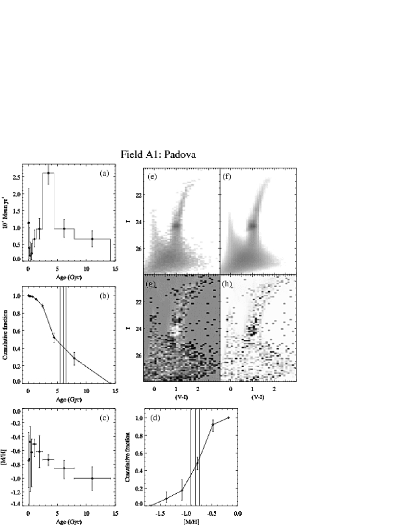
Figure 1.— SFH results for A1 using the Padova tracks (see text for details).

Figure 2.— Same as Fig. 1 but for A2.

Figure 3.— Same as Fig. 1 but for A3.

Ideally, we would work entirely in the native ACS/WFC filter system. IAC-STAR has an HST bolometric correction library from Origlia & Leitherer (2000) but it does not include $F606W$ and, strictly speaking, it applies only to WFPC2. As discussed in Sirianni et al. (2005) the WFPC2 and ACS filter transmission curves are not identical. Thus, we are forced to work in the $UBVRI$ system using the synthetic transformation of Sirianni et al. (2005). In our experience thus far, we have found good agreement between HST and ground-based data in the $UBVRI$ system for several Galactic globular clusters with [Fe/H] $\lesssim-1.5$. Mackey, Payne & Gilmore (2006) found no significant systematic errors after transforming to the ground-based system ACS/WFC photometry of two clusters in the Large Magellanic Cloud with metallicities similar to the majority of our M33 stars ([Fe/H] $\sim-1.0$) although it should be noted they used $F555W$ rather than $F606W$.

At higher metallicities the situation could be different. Our investigations have found tentative evidence for a constant offset of $\sim-0.05$ mag in $V$ when comparing 47 Tuc ([Fe/H] $\approx-0.7$) ACS photometry to independent ground-based data. On the RGB, this offset translates into an uncertainty of $\sim 0.1$ dex and $\sim 1.5$ Gyr at a metallicity of $-1.0$. This offset is equal to the uncertainty of the photometric zero-point of the Sirianni et al. synthetic transformation. Considering our coarse binning scheme in age, metallicity, and in the CMD plane (as defined below) and given that a large fraction of our M33 stars have metallicities less than 47 Tuc we believe that any such offset is likely to have a small effect on our results especially when compared to the effect of uncertainties in the theoretical stellar evolutionary tracks themselves. We confirm this assertion in the Appendix where we fit a test population after manually inserting a V mag offset.

We employed StarFISH (Harris & Zaritsky 2001) to simulate the effects of observational errors in the synthetic CMDs and to search for the best-fit model CMD. The artificial star tests described in Paper I allow us to accurately quantify the photometric errors and completeness rate as functions of both magnitude and color. Each model star is associated with a nearby artificial star. If the artificial star was recovered its magnitude shifts are assigned to the model star otherwise the model star is discarded. Each synthetic CMD contains $\approx 1\times 10^{6}$ stars before the simulation of observational errors.

The coefficients in the linear combination of synthetic CMDs are proportional to the star formation rates (SFRs) at their respective ages and metallicities. StarFISH uses a downhill simplex algorithm to solve for the coefficients by minimizing a fitting statistic. We refer the reader to Harris & Zaritsky (2001) for more details of the algorithm. The model and data CMDs are divided into square bins 0.1 mag on a side and the number of model and data stars in each bin go into calculating the fitting statistic. This statistic is the negative log-likelihood ratio for a Poisson distribution given by $\Upsilon=2\sum_{i}m_{i}-n_{i}+n_{i}{\rm ln}(n_{i}/m_{i})$ where $m_{i}$ and $n_{i}$ are the number of model and data stars in CMD bin $i$, respectively. The properties of this parameter have been discussed in various studies (e.g., Mighell 1999; Hauschild & Jentschel 2001; Dolphin 2002). For large $m_{i}$ it is well approximated by the commonly used $\chi^{2}$.

Included in the linear combination of synthetic CMDs is a bad-point CMD which we fit to cosmic rays, hot pixels, foreground stars, and other objects in the observed CMD that cannot be reproduced by IAC-STAR (see also Dolphin 2002). This has the form of a uniform distribution that contributes $\sim 0.05$ “stars” to each CMD bin resulting in $\sim 120$ over the entire CMD. It also has the benefit of preventing $\Upsilon$ from diverging when $m_{i}=0$ and $n_{i}>0$.

Following Gallart et al. (1999) and Wyder (2001), the global best-fit model is the weighted average of all acceptable individual solutions, each of which corresponds to a particular combination of distance and reddening. A solution is acceptable if it lies within $1\sigma$ of the best-fit. For each individual solution StarFISH calculates the errors on the SFRs by moving through the parameter space in many different directions until the fitting statistic changes by $1\sigma$. Thus, the errors represent uncorrelated and correlated errors between the amplitudes. The errors of the individual best-fit solution are added in quadrature with the spread of all acceptable solutions. In this way the errors of the global best-fit reflect correlations between age, metallicity, distance, and reddening.

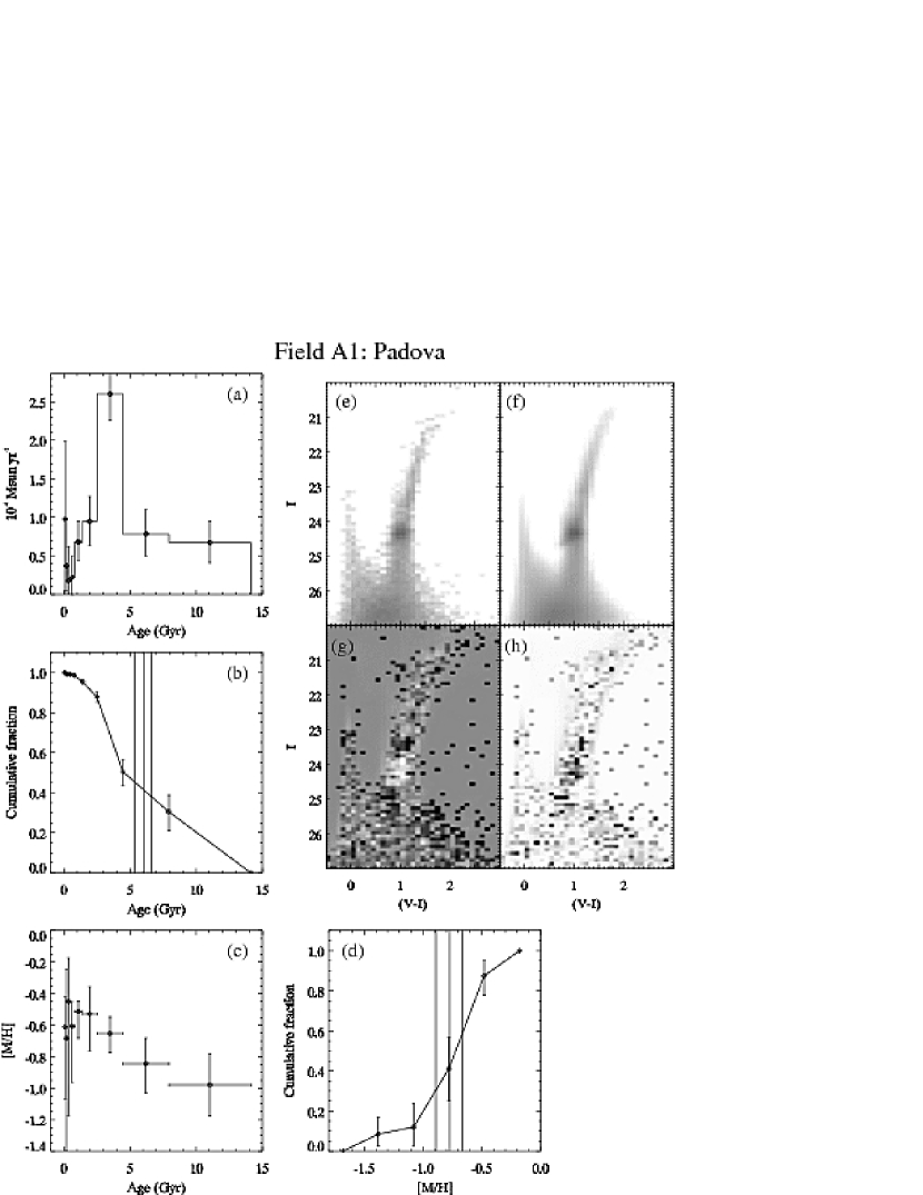
Figure 4.— SFH results for A1 using the Padova tracks and after excluding the region $I>27$ (see text for details).

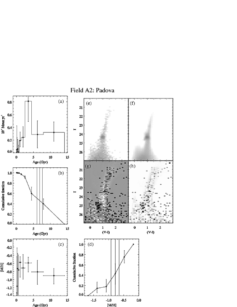
Figure 5.— Same as Fig. 4 but for A2.

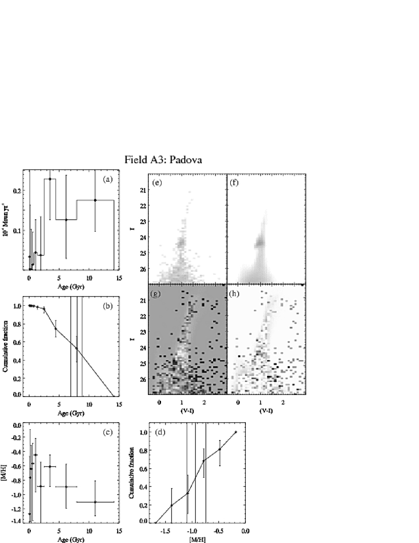
Figure 6.— Same as Fig. 4 but for A3.

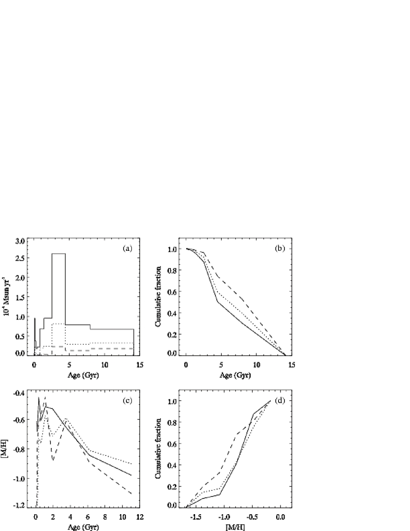
Figure 7.— Comparison of SFH results for A1 (solid), A2 (dotted), and A3 (dashed).

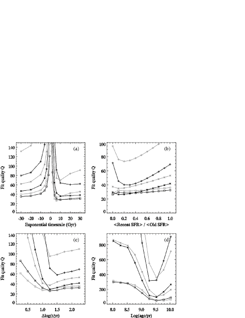
Figure 8.— Exploring parameter space by hand. Each graph shows how the fit quality varies with (a) exponential timescale, (b) ratio of mean recent SFR to old SFR, (c) star formation duration, and (d) age bin. The point symbols are diamonds, asterisks, and squares for fields A1, A2, and A3, respectively. Gray lines show the result of decreasing the metallicity (see text for details).

The quality of the fit is measured by the parameter, $Q$, which is the difference between $\Upsilon$ and its expectation value in units of its standard deviation. The expectation value depends on the model but is approximately equal to the number of CMD bins contributing to the fit minus the number of free parameters which include any nonzero SFH amplitudes (typically $\approx 25$) plus distance and extinction. The $Q$ parameter measures the likeliness of the data being randomly drawn from the model (Dolphin 2002). Only for comparison purposes we also calculate $\chi^{2}$ of the best-fit defined by $\chi^{2}=\sum_{i}(n_{i}-m_{i})^{2}/m_{i}$. The reduced $\chi^{2}_{\nu}=\chi^{2}/\nu$ where $\nu$ is the number of significant CMD bins minus the number of free parameters. Studies applying the synthetic CMD fitting method to real stellar populations typically find values for $Q$ and $\chi^{2}_{\nu}$ in the range $\sim 1-5$ (Dolphin 2002; Harris & Zaritsky 2004; Gallart et al. 1999; Skillman et al. 2003; Dolphin et al. 2003; Wyder 2001, 2003).

In the Appendix we demonstrate the effectiveness of the method on several test populations. In particular, we examine how errors in the various input parameters affect the accuracy of the recovered SFH and how they contribute to systematic errors in the results. Such tests are critical to understanding the strengths and limitations of the method and how to interpret the results.

3. Results

3.1. Padova tracks

Figures $\ref{fig:A1_padova_bad}-\ref{fig:A3_padova_bad}$ present the results using the Padova tracks. In each figure, panel (a) shows the SFH and $1\sigma$ errors as explained before. In panel (b) we show the age cumulative distribution function (age-CDF). Panel (c) displays the age-metallicity relation (AMR) where each point is the mean metallicity of all stars formed in the corresponding age bin. The horizontal errors denote the age bin width. Panel (d) is the metallicity cumulative distribution function (Z-CDF) of all stars ever formed. The vertical lines in panels (b) and (d) correspond to the mean age and metallicity of all stars and stellar remnants and the $1\sigma$ confidence intervals. Also shown are the data CMD (e), model CMD (f), residuals (g), and significance (h). The data and model CMDs are Hess diagrams (2-D histograms) on a logarithmic scale. The residuals are on a scale where $-3\sigma$ is black and $+3\sigma$ is white and positive residuals mean the model is too high.

Upon inspection of the solutions, we see that the model CMDs underpredict the number of stars fainter than $I=27$. This indicates an approximately constant number of contaminants at $I>27$ due to non-stellar sources like unresolved background galaxies and spurious noise artifacts. This contamination is much less than the number of real stars in A1 but becomes more significant in A2 and A3. The Teramo CMDs showed the same discrepancy making it unlikely that the stellar tracks are the cause. As a test we repeated the entire photometric reduction procedure and artificial star tests for A3 using more stringent detection requirements. This allowed us to repeat the SFH analysis for A3 which we found to yield better agreement between the model and data CMDs but the model still slightly underpredicted the number of stars at the faint end. The resulting SFH was nearly identical to that produced after excluding $I>27$ in the original dataset (see below) because there is little information there anyway to constrain the solution. Since this region is also beyond the $50\%$ completeness level, we will exclude it for the remainder of the analysis.

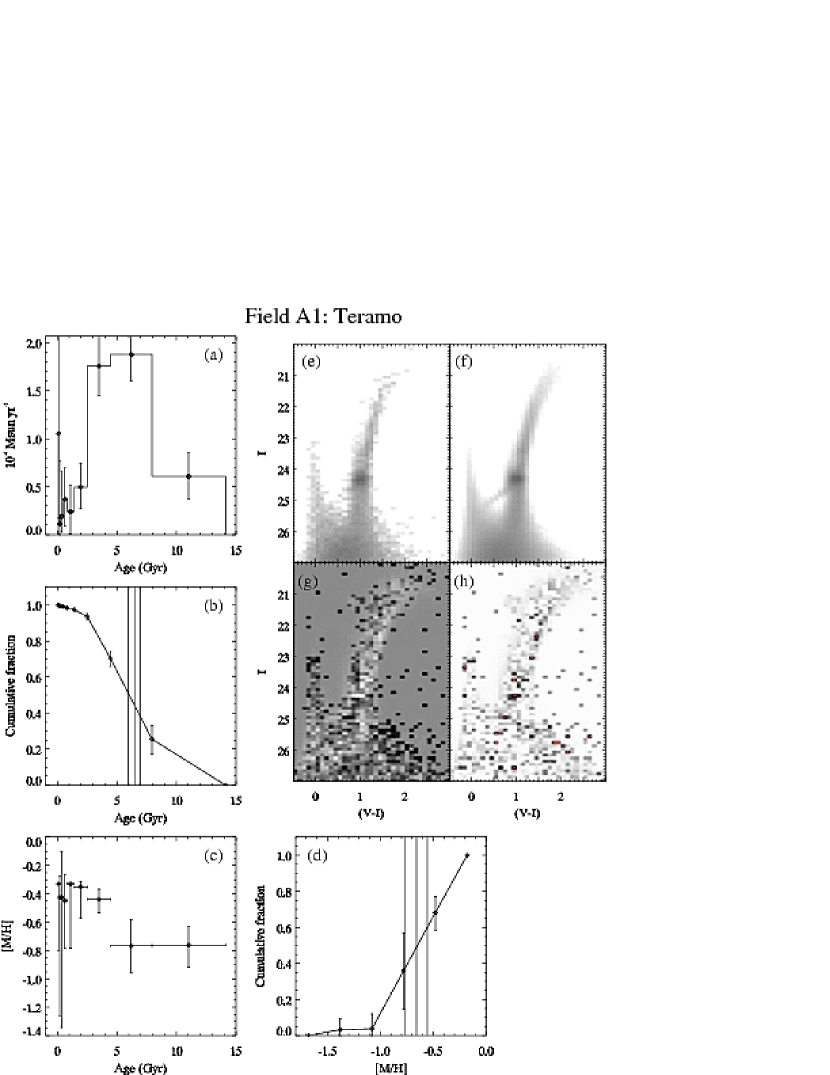
Figure 9.— SFH results for A1 using the Teramo tracks (see text for details).

Figure 10.— Same as Fig. 9 but for A2.

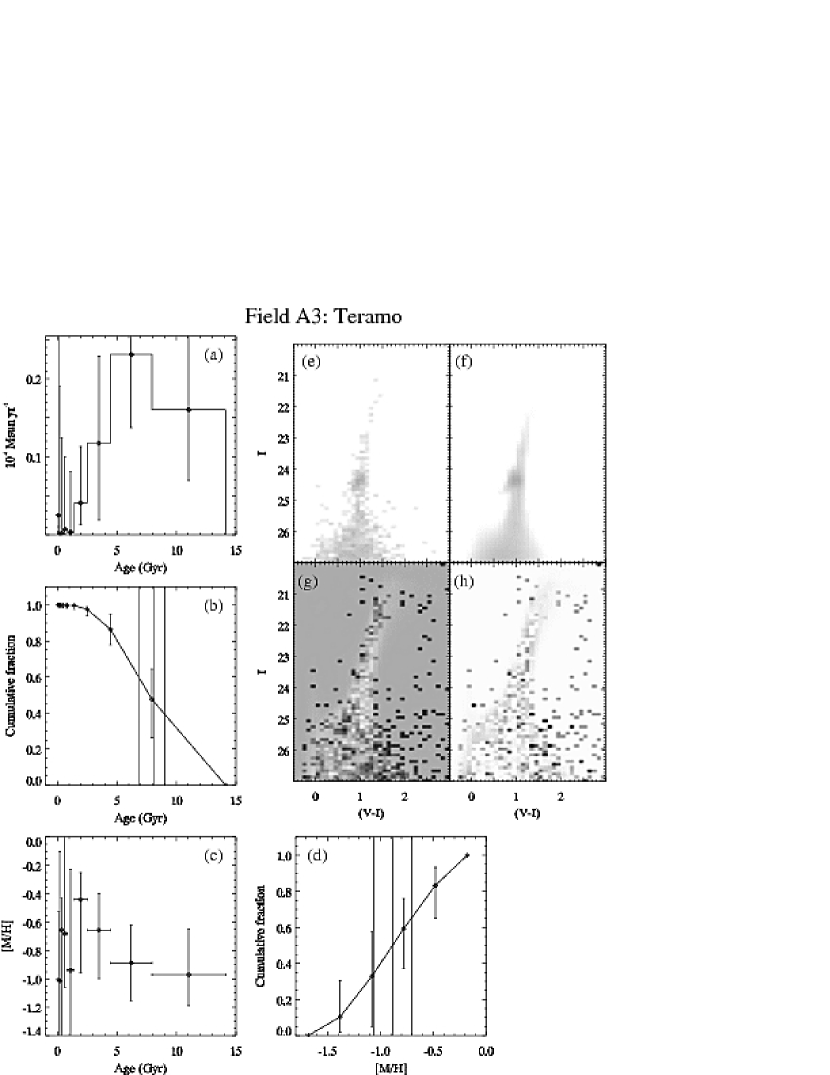
Figure 11.— Same as Fig. 9 but for A3.

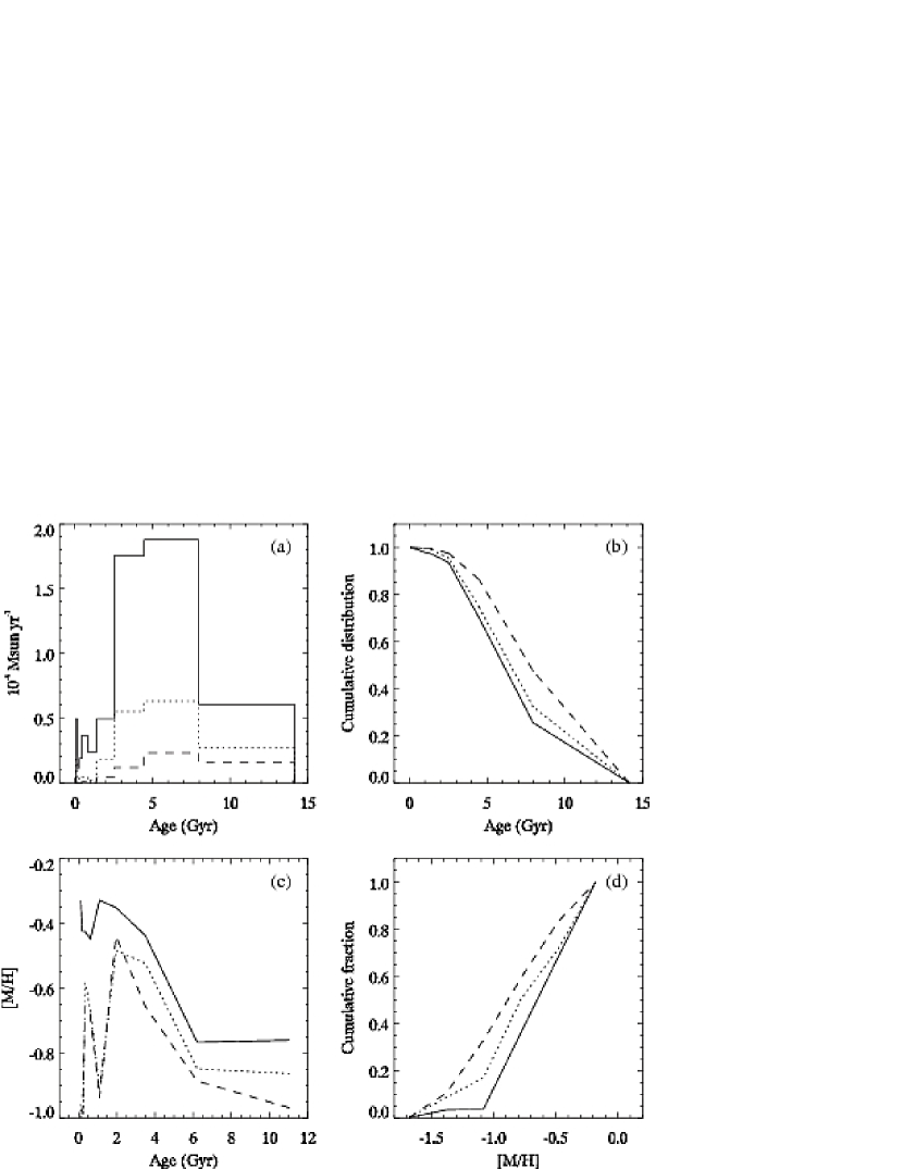
Figure 12.— Same as Fig. 7 but for the Teramo tracks.

Figure 13.— Same as Fig. 8 but for the Teramo tracks.

The new solutions are displayed in Figures  $\ref{fig:A1_padova}-\ref{fig:A3_padova}$. The largest discrepancies occur in the red clump (RC) and HB where the model overpredicts the number of stars. Disagreements in the RC and HB are common (e.g., Dolphin et al. 2003; Wyder 2001, 2003) due to uncertainties in the stellar evolutionary tracks. In A1 and A2, the model also underpredicts the number of stars just above the RC possibly indicating a problem with the AGB bump. In A3 these discrepancies are not as significant which could reflect a less complex SFH relative to A1 and A2.

Table 1 gives the fit quality and mean distance and extinction for each field together with their $1\sigma$ uncertainties. Table 2 lists the mean age, metallicity, and V-band mass-to-light ratio ($M/L_{V}$) with their $1\sigma$ uncertainties. Tables 3 $-$ 6 provide the SFH, age-CDF, AMR, and Z-CDF of the solutions.

To facilitate comparison between the three fields we show their results together in Figure 7. In each graph, A1 is the solid line, A2 the dotted line, and A3 the dashed line. The error bars have been omitted for clarity but they are the same as in Figs. $\ref{fig:A1_padova}-\ref{fig:A3_padova}$. The SFHs are qualitatively similar which is not surprising since the CMDs are similar, too. Field A1 shows an enhancement in the SFR during the period 2.5 $-$ 4.5 Gyr ago by a factor of $\sim 3-4$ over the mean SFR at older ages. Because of the large age bins employed, this does not necessarily mean the true SFH peaked at these exact ages (see Appendix). This is followed by a decline in the SFR toward younger ages until 250 Myr ago at which time the SFR increases. This might suggest a burst of star formation (SF) in the last 250 Myr but the youngest few age bins are dominated by small number statistics so the SFRs are not well constrained (see Appendix). More importantly, the SFR in the youngest few age bins could be overestimated if there are stars present in the data with ages $\lesssim 80$ Myr, the youngest age covered in the synthetic CMDs. For example, if the true SFR over the past $\sim 140$ Myr has been constant then the SFR in the youngest bin could be overestimated by a factor of $\sim 2$ to account for the stars formed over the last 80 Myr. Because of the correlations between age bins some of this overestimation may leak into nearby bins. Hence, the SFRs in the youngest $1-3$ bins should be viewed as upper limits.

A2 shows a similar behavior but the mean SFR at ages $<5$ Gyr is smaller relative to older ages. The enhancement at $\sim 3$ Gyr in A1 and A2 is almost nonexistent in A3. Indeed, the SFH of A3 is consistent with a constant SFR at ages $>2.5$ Gyr. The age-CDFs demonstrate more clearly that the fraction of stars formed prior to 4.5 Gyr ago increases from $\sim 50\%$ in A1 to $\sim 75\%$ in A3. The mean age of all stars ever formed increases from $6.09^{+0.59}_{-0.67}$ to $7.99^{+0.86}_{-0.98}$ Gyr. The mean metallicity decreases from $-0.77^{+0.11}_{-0.12}$ to $-0.93^{+0.19}_{-0.16}$.

In all three fields, the mean metallicity of forming stars increases in the oldest three age bins and then fluctuates wildly at younger ages. The fluctuations are smallest in A1 and largest in A3 suggesting they are the result of small number statistics at ages $\lesssim 2$ Gyr which contribute only $\lesssim 5\%$ to all stars in A2 and A3 (see Appendix). It is more instructive to average the metallicity at these young ages. When we do this we find that the mean metallicity for ages $\leq 2.5$ Gyr is $-0.53$, $-0.67$, and $-0.69$ with a standard error in the mean of $\approx 0.07$ dex. Hence, we can say with $95\%$ confidence that the mean metallicity of A1 at young ages is higher than that in A2 and A3 but A2 is consistent with A3.

As a consistency check on the solutions we can explore the parameter space by hand using the synthetic CMDs with $(m-M)_{0}=24.60$ and $A_{V}=0.20$. Panel (a) of Figure 8 shows what happens to the fit quality, $Q$, when we adopt an exponentially decreasing or increasing SFH and vary the timescale, $\tau$. Positive (negative) timescales correspond to a decreasing (increasing) SFR since formation time. The diamonds, asterisks, and squares represent A1, A2, and A3, respectively. For each field we have set $\tau=1,2,4,6,10,20$, and 30 and we normalize the model CMD to have the same total number of stars as the data CMD in the fitted region. The black lines correspond to synthetic CMDs with metallicities $\rm[M/H]=-0.8$ to $-0.5$ while the gray lines show the effect of using the next lowest metallicity bin, $\rm[M/H]=-1.3$ to $-1.0$.

The lowest $Q$ values in panel (a) are much larger than the global best-fit SFHs suggesting that the true SFH (averaged over our age bins) has not exactly followed an exponential throughout M33’s lifetime. Nevertheless, the preferred timescale decreases from $\sim 20$ Gyr in A1 to $\sim 6$ Gyr in A3. The difference in fit quality between exponentially increasing and decreasing SFHs with the same timescale is mainly sensitive to the mean SFR over the past $\sim 1$ Gyr. Ages $\lesssim 1$ Gyr contribute mostly to the CMD at colors $(V-I)\lesssim 0.5$ while the opposite is true for older ages. Exponentially increasing SFHs have many more stars at these blue colors than are observed in the data CMDs. The fact that exponentially decreasing SFHs are preferred indicates that the average SFR in the past $\sim 1$ Gyr has been lower than at older ages.

We explore this fact further in panel (b) which shows the ratio between the average recent SFR (ages $<794$ Myr) to the average SFR at older ages. The SFR in both regimes has been set constant and the ratio was varied in increments of 0.1. In A1 there is an unambiguous minimum at $0.2-0.3$, in A2 the minimum is less significant but occurs at $0.1-0.2$, and in A3 there is little constraint although the minimum occurs at 0.0. This supports the idea that, at least in A1 and A2, the mean SFR over the past $\sim 1$ Gyr has been lower than at older ages. The precise value of the ratio could depend on the shape of the true IMF relative to that of the model. For example, a model IMF with a single slope that is steeper (shallower) than in the data will cause an overestimate (underestimate) of the recent SFR because more young, high-mass stars will be needed to match the observations (Dolphin 1997).

Panel (c) explores the duration of star formation for a constant SFR starting at $\rm log(t/yr)=10.15$ (14.1 Gyr). The duration is successively increased in steps of 0.25 dex. We see that the optimal duration is 1.5 dex in A1 and 1.25 dex in A2 and A3. This further supports the case for a longer era of star formation in A1 than in A3.

In a similar manner we can also see what particular age range is preferred by comparing each individual synthetic CMD to the data CMD. We plot the results of this exercise in panel (d). This plot demonstrates that the synthetic CMD centered on log(age/yr) = 9.525 (age range $\approx 2.5-4.5$ Gyr) generally provides the closest match to the observed CMDs with a modest dependence on metallicity due to the age-metallicity degeneracy. Interpolating smoothly between the points by eye, it appears that the preferred age increases from A1 to A3 providing yet another confirmation that the mean age increases throughout the fields. Since the lowest $Q$ values are still very high we can conclude that SF has occurred over timescales longer than those covered in each of the synthetic CMDs alone. Overall, Fig. 8 makes it easier to understand the global best-fit solutions for A1 and A2 which show an enhancement in the SFR at $2.5-4.5$ Gyr with approximately constant SFR at other ages and a drop in the average SFR over the past 1 Gyr.

3.2. Teramo tracks

Figures $\ref{fig:A1_teramo}-\ref{fig:A3_teramo}$ display the global solutions obtained with the Teramo tracks. There are several striking differences between the Teramo and Padova solutions. First, the enhancement at intermediate ages occurs over two contiguous age bins from $\sim 2.5-8$ Gyr rather than just one bin. In A1, the strength of the enhancement is about $70\%$ smaller since it lasts for a longer timespan and the total number of stars must be conserved. In addition, a larger fraction of stars formed by 5 Gyr ago – $\sim 70\%$ as opposed to $\sim 50\%$ for the Padova tracks.

Another difference between the Teramo and Padova solutions is that the RC area in the Teramo model CMD provides a better fit to the data. Interestingly, though, the model has an extended blue HB which is not as obvious to see in the data. The Teramo models have a noticably more extended HB at old ages than the Padova models (Gallart et al. 2005). Although the extended HB does not appear to significantly constribute to the residuals, the large width of the oldest age bin may have forced the model to include very old stars ($\gtrsim 12$ Gyr) that might not be in the data. We re-ran the fitting routine but changed the oldest age bin to have a width of 0.15 dex so the oldest stars included in the model were 11.2 Gyr old. As expected, the HB morphology of the resulting fits was redder and similar to the Padova results in the previous section but the fit qualities were no better and the SFH was not significantly changed.

One notable difference between the Teramo model CMDs and data CMDs is that the models contain an excess of stars on the RGB. This is a known issue with the Teramo models which predict RGB lifetimes that are too long. This results in an RGB luminosity function with too many stars when compared to other sets of models and GGCs (Gallart et al. 2005). Since this discrepancy does not affect the color of the RGB it probably has little impact on our results.

We note that the best-fit distance modulus is $\sim 0.1$ mag greater for the Teramo tracks than for the Padova tracks yet the best-fit extinction values are similar. This underscores the fact that distances and extinctions obtained with this technique are subject to systematic errors in the stellar evolutionary tracks. These errors can depend on filter, age, and metallicity among other factors (Wyder 2003).

The Teramo solutions are overplotted on each other in Figure 12. Despite the differences from the Padova solutions, they exhibit similar trends between the three fields. The strength of the enhancement at intermediate ages decreases relative to the SFR at older ages. Consequently, the mean age of the fields increases from $6.50^{+0.46}_{-0.51}$ Gyr in A1 to $8.09^{+0.97}_{-1.24}$ Gyr in A3. The mean metallicity decreases from $-0.66^{+0.11}_{-0.11}$ to $-0.89^{+0.18}_{-0.18}$. The apparent lack of evolution in the AMR between the two oldest bins does not necessarily weaken the validity of the model nor does it necessarily mean there was no change in the true AMR. As shown in the Appendix, variations between adjacent bins must be considered with caution.

Figure 13 shows again that the Teramo tracks predict similar trends between the fields as the Padova tracks although some specific details are different. The preferred exponential timescale decreases from 10 Gyr in A1 to $4-6$ Gyr in A3. The ratio of recent SFR to past SFR is $0.1-0.2$ in A1 and consistent with zero in A2 and A3. The duration of star formation decreases from $1-1.3$ dex in A1 to $0.7-1.0$ dex in A3. Finally, the preferred age increases from log(age/yr) $=9.5$ in A1 to log(age/yr) $=9.8$ in A3.

4. Discussion

There have been few studies of the resolved stellar populations in the outer regions of late-type spiral galaxies. Davidge (2003) imaged the outskirts of M33 and NGC 2403 with the Gemini Multi-Object Spectrograph (GMOS) on Gemini North covering deprojected radii of $14-17$ kpc and $7-19$ kpc, respectively. He found evidence for bright RGB and AGB stars well mixed throughout the observed fields and interpreted them as evidence for in-situ SF at intermediate ages. Bland-Hawthorn et al. (2005) used the GMOS on Gemini South to observe the outskirts of another late-type spiral, NGC 300. Using star counts in the $r^{\prime}-$band, they found the exponential disk to extend out to $R_{dp}=14.4$ kpc or 10 optical scale lengths. Seth et al. (2005) studied the vertical distribution of resolved stars in six low-mass spiral galaxies and found the stellar component to extend up to 15 scale heights. Our results complement these other studies well and together they suggest that the stellar disk populations of late-type spirals commonly extend out to large distances. However, just because the stellar surface density or light distribution extends to these large distances does not necessarily mean the stars belong to a kinematic disk population (i.e., rotationally supported with ordered motion).

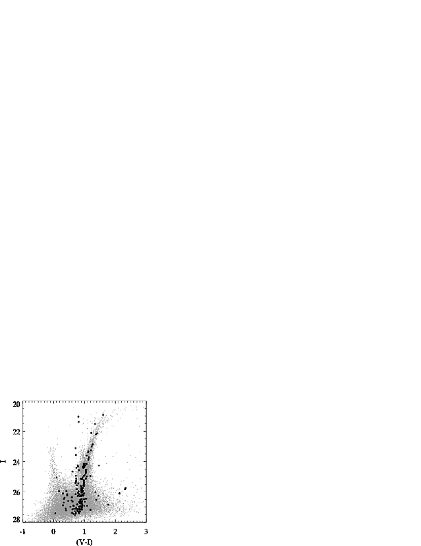
Figure 14.— CMD of field A1 (gray points) with CMD of Terzan 7 overplotted (black points).

An empirical check on our results is displayed in Figure 14. This figure shows the CMD of field A1 as gray points with the CMD of globular cluster Terzan 7 as black points. The Ter 7 data come from Sarajedini & Layden (1997) and we have plotted only stars within the central $80\arcsec$ of the cluster center. Most of the black points bluer than $(V-I)\sim 0.8$ are Galactic field stars. Ter 7 belongs to the Sagittarius dwarf galaxy and is estimated to have a metallicity [Fe/H] $=-0.82\pm 0.15$ and to be $\sim 6$ Gyr younger than 47 Tuc (Sarajedini & Layden 1997). The RC and RGB of Ter 7 closely match those of M33 confirming our general result that M33’s outskirts are $6-8$ Gyr old with metallicities of $\sim-0.7$ to $-0.9$.

Ciardullo et al. (2004) conducted a photometric and spectroscopic survey of planetary nebulae (PNe) throughout M33. They estimated the disk mass surface density under the epicyclic and isothermal disk approximations by combining the vertical velocity dispersions of the PNe with published optical surface photometry and gas mass surface densities. To account for extinction they adopted the simple exponential model of Regan & Vogel (1994) with a central $A_{V}$ of 0.9. Ciardullo et al. found that $M/L_{V}$ of the stellar component increases from $\sim 0.3$ to $\sim 1.5$ over the face of the disk. We show their results as squares in Figure 15 after transforming to a Galaxy-M33 distance of 867 kpc (Paper I; Galleti et al. 2004). The $M/L_{V}$ values for fields A1 $-$ A3 derived from our SFH analysis are shown as circles (Padova) and triangles (Teramo).

This provides a nice consistency check on our SFH results because $M/L_{V}$ depends heavily on age and to a lesser extent on metallicity. For instance, the Padova synthetic CMDs covering metallicities from $-0.8$ to $-0.5$ have an $M/L_{V}$ that increases with age from 0.16 to 3.57. The relative proportions of different ages in the SFHs affect both the normalization of $M/L_{V}$ and its change with radius. The agreement between the two sets of data thus provides independent support that our SFH results contain a reasonable mix of ages and metallicities.

More fundamentally, the agreement supports the IMF we used in calculating the SFHs. Recall that the low-mass exponent ($M\leq 0.5\ M_{\sun}$) was $-1.35$. If we steepen it to $-2.00$ then $M/L_{V}$ increases by $\sim 20\%$ without affecting the SFHs. A flatter low-mass slope of $-0.70$ would decrease $M/L_{V}$ by $\sim 10\%$. Changing the IMF slope at higher masses could affect the SFHs and resulting $M/L_{V}$ in a non-trivial way. However, it is unlikely that we just happened to pick a particular form of the IMF which yields a similar $M/L_{V}-R_{dp}$ relation as the PNe kinematics. Therefore, it seems that the IMF in M33’s outskirts is similar to the Galaxy’s or is at least shallower than a Salpeter form at the lowest masses.

Taken at face value, Fig. 15 also suggests that the mean age of M33’s entire stellar disk increases with radius. All else being equal, the correlation between age and $M/L$ is one-to-one for simple stellar populations but late-type galaxies like M33 are characterized by SF at a wide variety of ages. In systems where SF has occurred in the last $\sim 1$ Gyr, the light from the most massive, youngest stars can completely overwhelm the light from older stellar generations thus weakening or even reversing the correlation between $M/L$ and mean age. This is because while the youngest stars contribute the majority of the light they have only a small effect on the age averaged over a Hubble time. Therefore, it may be premature to extrapolate the positive age gradient in M33’s outer disk to its inner disk. In future work, we will examine the SFH of M33’s inner disk to shed further light on this issue.

An increasing mean age in M33’s disk is apparently at odds with the inside-out scenario of galaxy formation. There is a wide body of theoretical and observational evidence to support the inside-out scenario. It is a standard prediction of hierarchical disk galaxy formation models with cold dark matter (e.g., Fall & Efstathiou 1980; Mo et al. 1998). The sizes of disk galaxies are observed to decrease with redshift in rough accordance with model predictions (Ferguson et al. 2004). Furthermore, galactic disks in the local Universe generally become bluer with increasing radius which is usually interpreted as a decreasing mean age (e.g., de Jong 1996; Bell & de Jong 2000).

Does the inside-out build-up of dark matter halos necessarily result in stellar disks whose mean ages at the present epoch decrease with radius? The question is difficult to answer because it requires incorporating the highly uncertain physics of gas cooling, star formation, feedback, and the effects of an ionizing background into the results of hierarchical cosmological simulations (Silk 2003). Most theoretical predictions for the run of mean age with radius come from simplified analytic or semi-analytic treatments of the baryonic physics (e.g., Mollá & Díaz 2005; Naab & Ostriker 2006). These studies do predict the mean stellar age to decrease with radius under the inside-out hierarchical framework. However, the treatments of the processes may break down in the outskirts of disks or the various assumptions and neglected processes in these predictions could change the results. Perhaps the initial build-up of the disk proceeds quickly so that after a few Gyr there is a negative age gradient but subsequent processes like gas infall, outflow, and viscous radial flows reverse this gradient. Alternatively, star formation could begin in an inside-out fashion but it could be truncated outside-in producing a positive age gradient because the inner regions would be forming stars for a longer period of time.

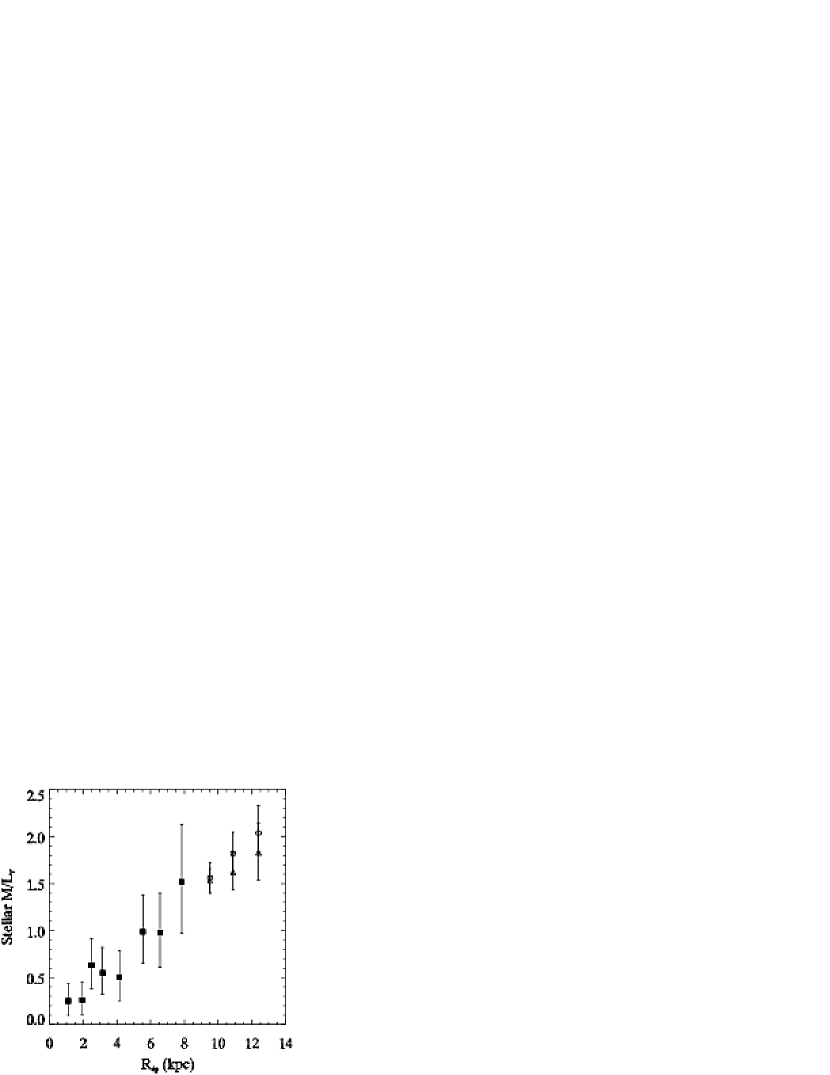
Figure 15.— V-band stellar mass-to-light ratio in M33. Squares represent the data based on PNe kinematics (Ciardullo et al. 2004). Circles and triangles correspond to the SFH results for fields A1 $-$ A3 using the Padova and Teramo models, respectively.

On the observational side, the nature, ubiquity, and interpretation of negative disk color gradients is not entirely clear. MacArthur et al. (2004) examined optical and near-IR color gradients for a large sample of galaxies and derived luminosity-weighted mean age and metallicity profiles from stellar population synthesis models. They found evidence for a radial dependence of age gradients in the sense that the inner regions showed generally steeper gradients than the outer regions. In addition, some galaxies displayed inflection points in their age gradients. Taylor et al. (2005) found a morphological dependence of color gradients such that early-type systems tended to get bluer with radius whereas late-type spiral, irregular, peculiar, and merging galaxies tended to get redder with increasing radius. They attributed this to mergers, accretions, and interactions triggering radial inflows of gas and centrally concentrated starbursts. They also found that galaxies with faint absolute B-band magnitudes were somewhat more likely to get redder with radius than their brighter counterparts. On the other hand, Jansen et al. (2000) found no color gradient dependence on morphological type but an even stronger trend with B-band magnitude. They concluded that star formation tends to occur in the outer regions of luminous galaxies but in the inner regions of fainter systems.

How does M33 compare with the results of the aformentioned studies? Because of its large angular extent in the sky and low surface brightness, M33’s color gradients are not well known. Guidoni et al. (1981) carried out $UBVRI$ photoelectric measurements of the central $13\arcmin$ and found the disk colors to change little with radius except for $(U-B)$ which is heavily influenced by dust. The 2MASS Large Galaxy Atlas (Jarrett et al. 2003) reports $(J-K_{S})$ as increasing from $\approx 0.8$ to 1.0 over the inner $9\arcmin$. Regan & Vogel (1994), on the other hand, found $(J-K)$ to decrease from $\approx 1.0$ to 0.8 over the same region. The cause of the discrepancy is not clear but it could arise from uncertainties in the sky subtraction. In any case, our SFH results predict instegrated colors of $(V-I)\approx 1.0$, $(B-I)\approx 1.7$, and $(J-K)\approx 0.8$ in M33’s outer disk. These values are in reasonable agreement with the published measurements but it would be worthwhile to update and extend the radial coverage of M33’s surface photometry. Such data could provide independent constraints on SFH analyses similar to our own.

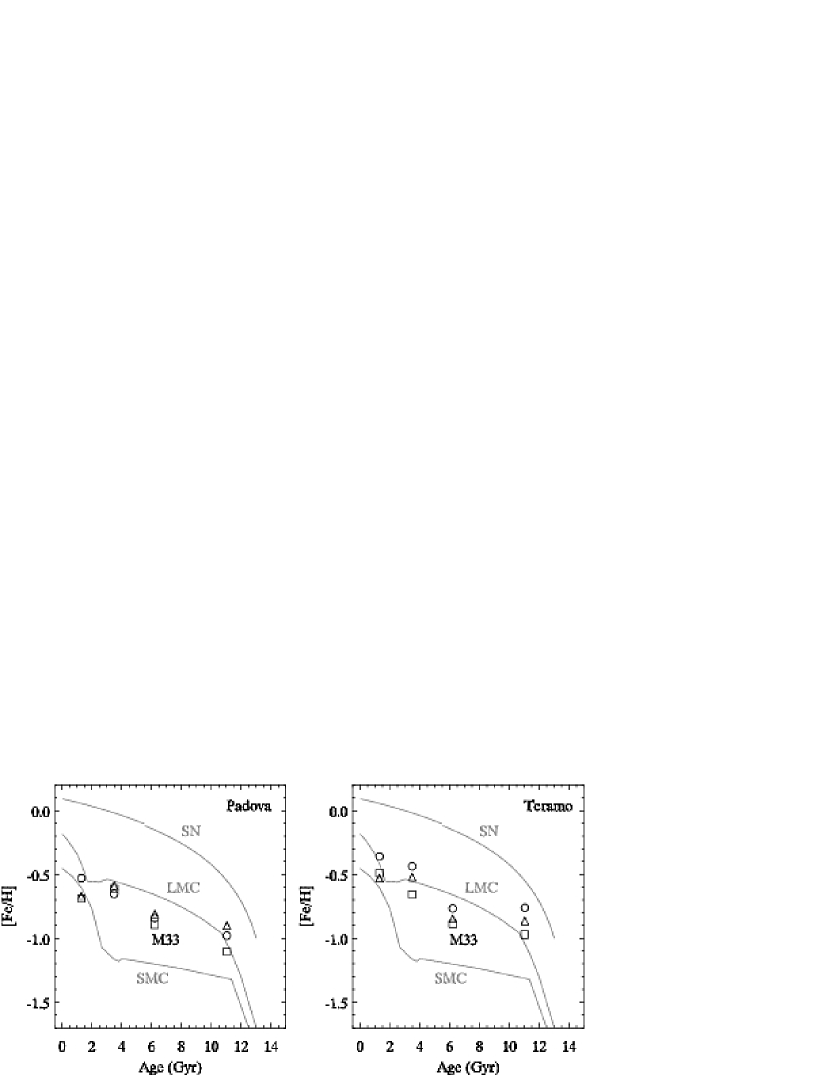
Figure 16.— AMR of M33 compared to the SN, LMC, and SMC shown as gray lines. Fields A1, A2, and A3 correspond to circles, triangles, and squares, respectively. The left panel shows the Padova results while the right panel shows the Teramo results (see text for details).

It is interesting to compare our results for M33’s AMR to that of other well-studied systems. In Figure 16, the gray solid lines show the AMRs of the Small and Large Magellanic Clouds (SMC and LMC, or MCs), and the Solar neighborhood (SN). For the MCs we have used the bursting models of Pagel & Tautvaišienė (1998) which include inflow and non-selective galactic winds. These authors tuned the parameters of their models to match the observed abundances of MC clusters and supergiants. The abrupt change in the enrichment rate at $\sim 3$ Gyr is due to a burst in star formation possibly caused by an interaction between the clouds. The SN model is taken from Twarog (1980) who used the abundances of a large sample of nearby F dwarfs as constraints. This model incorporated an initial metallicity of $-1.0$ and a constant SFR and inflow rate over the disk lifetime.

The existence and nature of an AMR in the SN is a matter of some debate. Edvardsson et al. (1993) and Feltzing et al. (2001) found the AMR to have a large intrinsic scatter ($\sim 0.2$ dex) with the oldest stars being both metal-poor and metal-rich. Subsequent studies have since challenged their results citing sample selection effects or biases in the age determinations as the cause (Garnett & Kobulnicky 2000; Rocha-Pinto et al. 2000; Kotoneva et al. 2002; Pont & Eyer 2004; Rocha-Pinto et al. 2006). In any case, we are concerned with the mean overall level of enrichment rather than the scatter and in this sense the Twarog AMR agrees well with most other studies (Rocha-Pinto et al. 2000).

The points in Fig. 16 show the AMRs we derived for field A1 (circles), A2 (triangles), and A3 (squares). The Padova results are shown in the left panel while the Teramo results are shown in the right panel. Because the AMR at the youngest ages is dominated by small number statistics, we have averaged the 6 youngest age bins which cover ages $\lesssim 2.5$ Gyr.

This figure demonstrates that the level of enrichment in M33’s outer disk has been intermediate between the SMC and LMC but perhaps somewhat closer to the latter. Indeed, if the SMC and LMC had continued to evolve quiescently rather than experience bursts at $\sim 3-4$ Gyr then their present-day metallicities would have been close to $-0.9$ and $-0.5$, respectively. In that case M33’s outer disk would have resembled the LMC even more.

Finally, our results imply a present-day global metallicity of $\sim-0.5$ in M33’s outer disk which is in good agreement with the results of Urbaneja et al. (2005). These authors conducted a detailed spectral analysis of $\sim 10$ B-type supergiant stars throughout M33 based on non-LTE model atmospheres including the effects of stellar winds. They found [M/H] in their stellar sample to decrease from about 0.0 near M33’s nucleus to about $-0.5$ at $R_{dp}=33\arcmin$ just interior to field A1.

5. Conclusions

We have conducted a detailed analysis of the SFH of M33’s outer regions by modelling the observed CMDs as linear combinations of individual synthetic populations with different ages and metallicities. To gain a better understanding of the systematic errors we have conducted the analysis with two different sets of stellar tracks, Padova and Teramo. The precise details of the results depend on which tracks are used but we can make several conclusions that are fairly robust despite the differences.

Both sets of tracks predict the mean age to increase and the mean metallicity to decrease with radius. When star formation is restricted to age intervals 0.25 dex wide and global metallicity intervals 0.3 dex wide, then ranges centered on ages $3-8$ Gyr and metallicities $-1.0$ to $-0.7$ are preferred with A1 matching more closely the younger, metal-rich ends of these ranges and A3 matching more closely the older, metal-poor ends. If star formation began at the same time in each field then its timescale has decreased with radius.

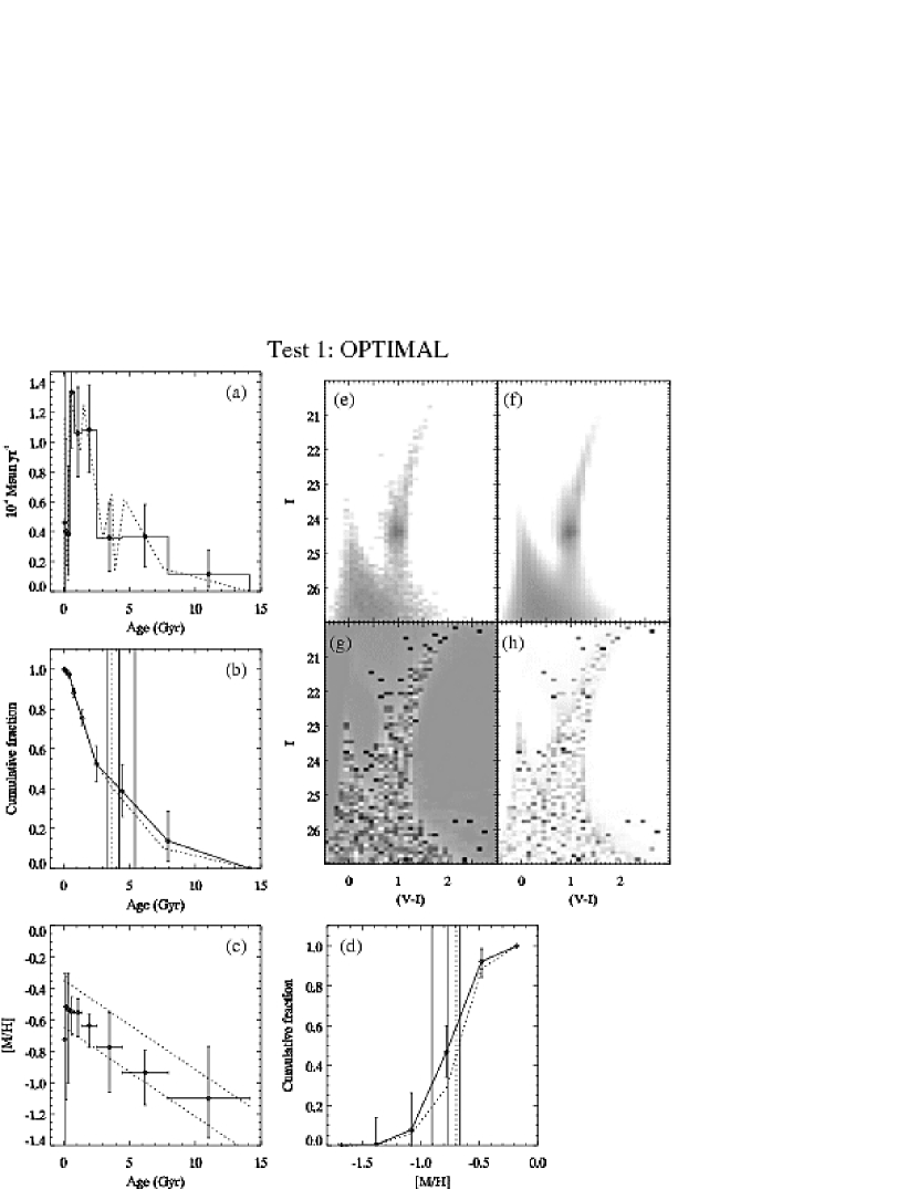
Figure 17.— Testing the method. Same panels as Fig. 4. See Appendix for details.

Figure 18.— Same as Fig. 17.

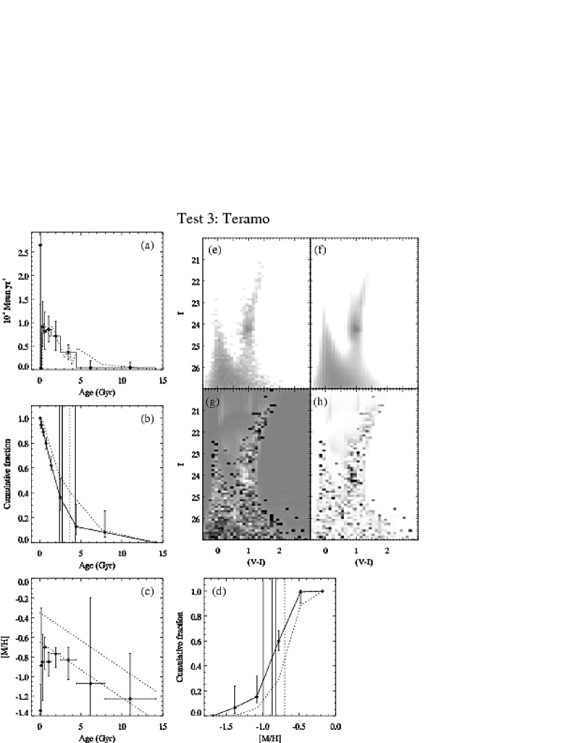
Figure 19.— Same as Fig. 17.

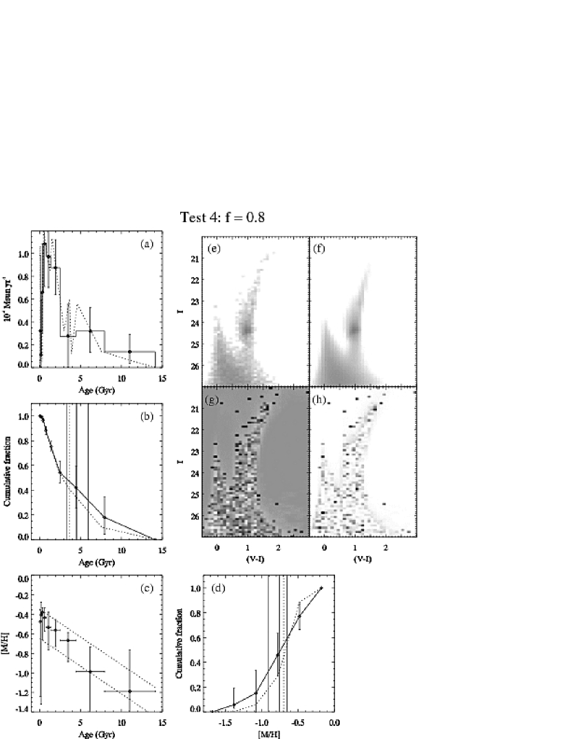
Figure 20.— Same as Fig. 17.

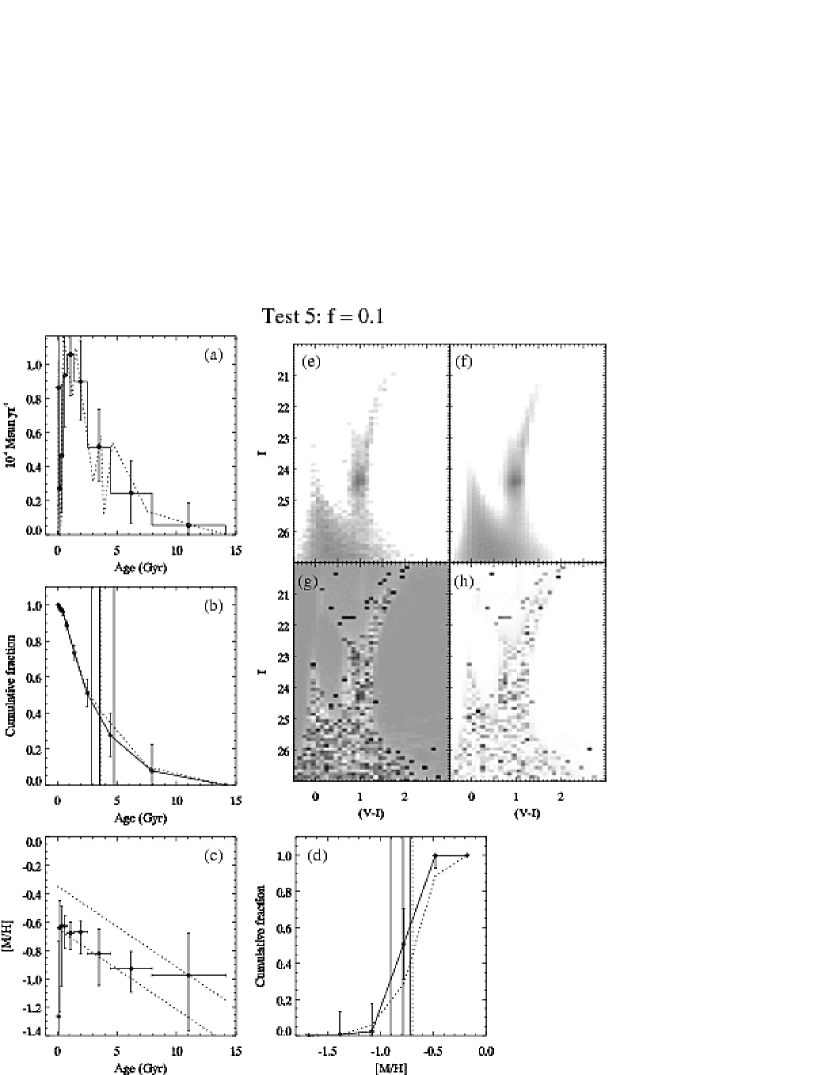
Figure 21.— Same as Fig. 17.

Figure 22.— Same as Fig. 17.

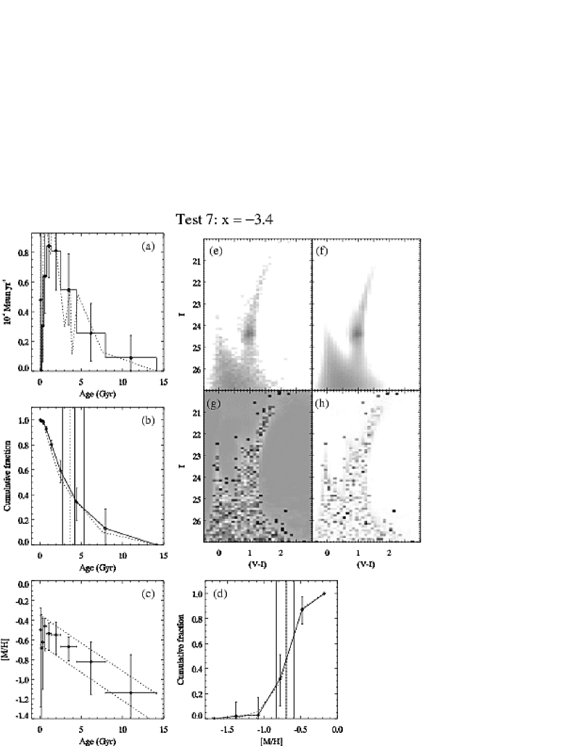
Figure 23.— Same as Fig. 17.

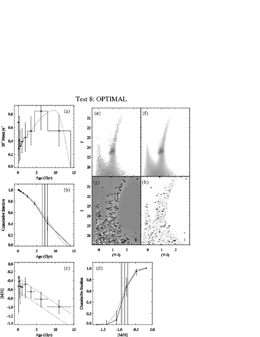
Figure 24.— Same as Fig. 17.

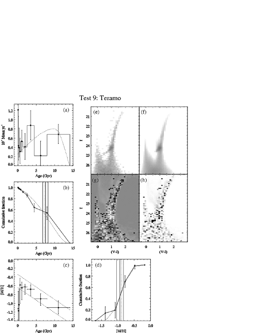
Figure 25.— Same as Fig. 17.

Figure 26.— Same as Fig. 17.

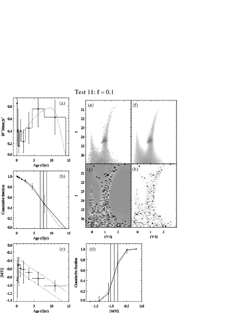
Figure 27.— Same as Fig. 17.

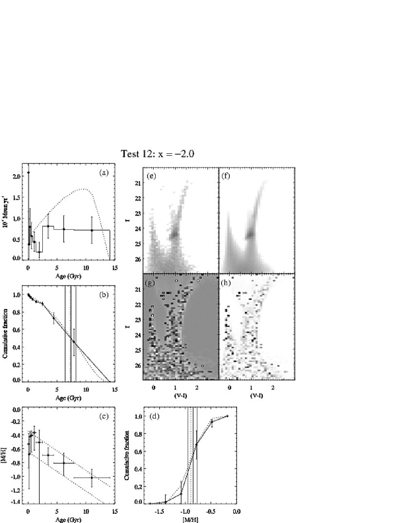
Figure 28.— Same as Fig. 17.

Figure 29.— Same as Fig. 17.

Figure 30.— Same as Fig. 17.

Figure 31.— Same as Fig. 17.

Figure 32.— Same as Fig. 17.

Allowing age and metallicity to vary as free parameters and assuming SF began $\sim 14$ Gyr ago, we find that, in A1, the mean SFR $80-800$ Myr ago was $\sim 30\%$ as high as the lifetime-averaged SFR, in A2 it was $\sim 10\%$ as high, and in A3 $\sim 5\%$ as high. Averaging the results from the Padova and Teramo tracks, the fraction of stars formed by 4.5 Gyr ago increases from $\sim 65\%$ in A1 to $\sim 80\%$ in A3. The mean age of all stars and stellar remnants increases from $\sim 6$ Gyr to $\sim 8$ Gyr and the mean global metallicity decreases from $\sim-0.7$ to $\sim-0.9$. The random errors on these age and metallicity estimates are $\sim 10\%$, 1.0 Gyr, and 0.1 dex. By comparing the results of the two sets of stellar tracks for the real data and for test populations with known SFH we have estimated the systematic errors to be $15\%$, 1.0 Gyr, and 0.2 dex. These do not include uncertainties in the bolometric corrections or $\alpha$-element abundances which undoubtedly deserve future study.

Simple linear least-squares fits to the mean ages and metallicities of all three fields yield an age gradient of $\rm 0.58\pm 0.27(rand)\pm 0.15(sys)\ Gyr\ kpc^{-1}$ and a metallicity gradient of $\rm-0.06\pm 0.05(rand)\pm 0.03(sys)\ dex\ kpc^{-1}$. This metallicity gradient is roughly consistent with that found in Paper II modulo an offset of $\sim 0.4$ dex. Half of this offset is due to the younger mean age of M33 compared to the GGCs and half is due to the lower $\alpha$-element abundance ([$\alpha$/Fe] = 0) of the stellar tracks (see also Salaris & Girardi 2005). We caution that the age and metallicity gradients do not necessarily continue into the inner disk. However, the stellar $M/L_{V}$ implied by our results is consistent with extrapolation of the independent estimates of Ciardullo et al. (2004) for regions interior to ours and together they imply that $M/L_{V}$ increases linearly over $\sim 6$ visual scale lengths, from $\sim 0.3$ at $R_{dp}=1$ kpc to $\sim 2.0$ at $R_{dp}=13$ kpc.

In Paper II we found that the stellar scale length increases with age in a roughly power-law fashion reminiscent of what has been observed in the vertical direction in six low-mass spirals (Seth et al. 2005). This behavior could be caused by the orbital diffusion of stars as they age. Therefore, the SFH we have derived in the present study could reflect a superposition of star formation and later dynamical processes which act to redistribute stars in the disk. Any similar analyses carried out on other stellar populations, especially those of disk galaxies, could face similar uncertainties.

6. Appendix

Here we provide a demonstration of the synthetic CMD-fitting method used in this paper by fitting many test populations with known SFHs. Each test population was generated in IAC-STAR with $q=0.60,(m-M)_{0}=24.68$, and $A_{V}=0.18$ and the SFR was normalized to produce $\approx 10,000$ observed stars. We varied the binary fraction ($f$), the slope of the IMF for masses above $1.0\ M_{\sun}$ ($x$), and the stellar tracks used to make the test populations. In all cases, the distance and extinction were fitted simultaneously with the SFH in the same manner as for the real data.

The results are shown in Figures $\ref{fig:test1}-\ref{fig:test16}$ where the figure titles tell the true value of the varied parameter. “Optimal” tests have the parameters held at their true values. All test populations were generated with the Padova tracks except for those titled “Teramo” which were generated with the Teramo tracks. The Padova synthetic CMDs were used to fit every test population. The panels in these figures are the same as in Fig. 1 but we also show the true SFH, age-CDF, AMR, and Z-CDF as dotted lines. The vertical dotted lines represent the true mean age and metallicity of all stars ever formed. Lastly, Table 7 lists the fit quality, distance, and extinction for each test.

In general, the agreement between the recovered SFH, distance, and extinction and their true values is good. The error bars are realistic indicators of the typical deviations. Even when the true binary fraction is as low as 0.1 or as high as 0.8 the solution is quite accurate. Errors in the high-mass IMF slope can cause normalization errors in the recovered differential SFRs yet the age-CDF, AMR, and Z-CDF are recovered accurately and there are no large residuals between the model and data CMDs. Therefore, the method is stable against reasonable errors in the binary fraction and IMF given the depth of our photometry.

Due to the relatively large age bins employed in the present analysis the peak in the recovered SFH can be significantly different from the peak in the true SFH. For example, even in the best-case scenario where all input parameters are correct, Test 8 shows that one could mistakenly conclude a peak in the SFR at ages $\sim 4.5-8.0$ Gyr when in fact the peak is at $9-10$ Gyr. Similarly, the large age bins limit the conclusions that can be made regarding the “burstiness” of the SFH. Any burst of shorter duration than the corresponding age bin will be distributed throughout the entire bin. Even in the optimal cases adjacent bins can have the same SFR or metallicity leading one to think that these quantities are constant when they are truly changing. Therefore, caution is required when interpreting bin-to-bin variations and more weight must be given to the net change over several bins. However, the age-CDF is recovered quite accurately and is relatively insensitive to errors in $f$ or $x$. Hence, conclusions based on the age-CDF are in general more robust than those based on the differential SFH (see also Holtzman 2001).

Since the age-sensitive sub-giant branch for ages $\gtrsim 5$ Gyr lies fainter than $I=27$, there is not as much information available to distinguish between the oldest two age bins. Therefore, these bins are more susceptible to the age-metallicity degeneracy and they should be considered with caution. The tests show that the largest deviations often occur in these bins but they are typically within the error bars.

Another important fact is that the youngest three points in the SFH and AMR can show significant errors even when the entire age-CDF and Z-CDF are reasonably recovered. This behavior arises from small number statistics in the CMD regions occupied by stars with the youngest ages. The metallicity has a small effect on the position of the bright MS and a much larger effect on the red supergiant and blue helium-burning phases (e.g., Dolphin et al. 2003) but if there are few stars populating the latter then the metallicity at ages $<1$ Gyr is hard to constrain.

The largest inaccuracies in the solutions come from errors in the stellar tracks. Tests 3 and 9 show that imperfections in the tracks can cause deviations larger than the $1\sigma$ errors although nearly all the deviations are $<2\sigma$. The CMD regions that are fit poorly may only contain a small range of ages or metallicities, thus affecting a small portion of the recovered SFH. The strong correlations between adjacent age/metallicity bins, though, may cause errors in one bin to leak into other bins. More importantly, there are multiple CMD regions with the same ages and metallicities so if one region is fit poorly then the others can still drive the solution toward a good fit (provided there are no errors in those other regions). The stellar tracks are more accurate at some ages and metallicities than others. Therefore, the accuracy of the recovered SFH depends on the true SFH itself.

We investigated several other CMD binning schemes for Tests 3 and 9 including 0.25 mag square bins and rectangular bins longer in the color dimension. We also tried masking out the RC region from the fits to see if that was the main source of error. In all cases the solutions were somewhat less accurate than in the original binning scheme. This agrees with the findings of Dolphin (2002) that increasing the CMD bin size decreases sensitivity and that the RC can contain vital age and metallicity information even when it is not perfectly modeled.

Finally, in the last test we have applied an offset of $-0.05$ mag to the V-band of the simulated data stars with $\rm[M/H]>-0.8$. Such a metallicity-dependent offset could arise from an imperfect transformation to the ground-based photometric system. The solution is almost unaffected. All quantities are recovered accurately. The only systematic error occurs in the AMR where the metallicitiy is underestimated by $\sim 0.1$ dex for $\rm[M/H]>-0.8$. Nevertheless, this difference is still within the $1\sigma$ errors of the solution.

These tests show that the method can reliably extract useful information such as the age and metallicity distributions of all stars ever formed. This holds even when the binary fraction and high-mass IMF slope are reasonably different from the values we have assumed. Errors in the tracks themselves make the largest contribution to our systematic errors which we can quantify by comparing the results (for the real data and test data) obtained with the Padova and Teramo tracks. We estimate conservative systematic uncertainties of $\pm 15\%$ in the age-CDF, $\pm 1.0$ Gyr in the mean age, and $\pm 0.2$ dex in the AMR and mean metallicity. These estimates do not include variations in the $\alpha$-element abundances or errors in the bolometric corrections.

Table 1Basic results of SFH solutions

Field	$Q$	$\chi_{\nu}^{2}$	$\nu$	$\overline{(m-M)_{0}}$	$\sigma$	$\overline{A_{V}}$	$\sigma$
Padova tracks
A1	6.64	1.70	1714	24.60	0.05	0.20	0.06
A2	3.98	1.57	1730	24.63	0.07	0.16	0.06
A3	2.81	1.66	1734	24.61	0.09	0.18	0.06
Teramo tracks
A1	6.02	1.68	1726	24.70	0.05	0.15	0.06
A2	3.55	1.53	1727	24.75	0.07	0.15	0.05
A3	2.99	1.68	1733	24.71	0.10	0.17	0.06

Table 2Basic results of SFH solutions

Field	$\overline{\rm Age}$	$\sigma_{hi}$	$\sigma_{lo}$	$\overline{\rm[M/H]}$	$\sigma_{hi}$	$\sigma_{lo}$	$\overline{M/L_{V}}$	$\sigma_{hi}$	$\sigma_{lo}$
	(Gyr)	(Gyr)	(Gyr)
Padova tracks
A1	6.09	0.59	0.67	-0.77	0.11	0.12	1.56	0.16	0.16
A2	6.87	0.76	0.83	-0.78	0.13	0.15	1.82	0.23	0.22
A3	7.99	0.86	0.98	-0.93	0.19	0.16	2.04	0.29	0.23
Teramo tracks
A1	6.50	0.46	0.51	-0.66	0.11	0.11	1.53	0.13	0.13
A2	7.00	0.68	0.75	-0.77	0.10	0.13	1.62	0.20	0.19
A3	8.09	0.97	1.24	-0.88	0.18	0.18	1.83	0.31	0.29

Table 3SFH of M33’s Outer Regions

Age Range	A1			A2			A3
log(yr)	$SFR$	$\sigma_{hi}$	$\sigma_{lo}$	$SFR$	$\sigma_{hi}$	$\sigma_{lo}$	$SFR$	$\sigma_{hi}$	$\sigma_{lo}$
Padova tracks
9.90–10.15	0.673	0.276	0.262	0.320	0.165	0.140	0.176	0.104	0.078
9.65– 9.90	0.783	0.318	0.290	0.286	0.218	0.209	0.126	0.112	0.097
9.40– 9.65	2.601	0.345	0.336	0.810	0.327	0.320	0.229	0.120	0.102
9.15– 9.40	0.950	0.322	0.319	0.241	0.172	0.154	0.037	0.097	0.037
8.90– 9.15	0.680	0.261	0.235	0.192	0.133	0.099	0.044	0.082	0.044
8.65– 8.90	0.220	0.283	0.220	0.010	0.109	0.010	0.014	0.082	0.013
8.40– 8.65	0.175	0.437	0.171	0.058	0.154	0.033	0.001	0.101	0.001
8.15– 8.40	0.371	0.609	0.318	0.013	0.228	0.013	0.001	0.162	0.001
7.90– 8.15	0.978	1.012	0.611	0.047	0.378	0.047	0.034	0.279	0.034
Teramo tracks
9.90–10.15	0.606	0.252	0.229	0.272	0.161	0.134	0.160	0.109	0.091
9.65– 9.90	1.877	0.284	0.271	0.633	0.159	0.146	0.231	0.107	0.094
9.40– 9.65	1.756	0.325	0.313	0.550	0.231	0.224	0.117	0.112	0.098
9.15– 9.40	0.495	0.247	0.223	0.178	0.114	0.094	0.041	0.072	0.028
8.90– 9.15	0.241	0.275	0.235	0.022	0.112	0.020	0.003	0.077	0.003
8.65– 8.90	0.367	0.335	0.277	0.047	0.131	0.047	0.007	0.093	0.006
8.40– 8.65	0.191	0.471	0.164	0.045	0.176	0.024	0.002	0.123	0.002
8.15– 8.40	0.115	0.655	0.115	0.001	0.245	0.001	0.001	0.189	0.001
7.90– 8.15	1.052	1.121	0.881	0.014	0.386	0.014	0.025	0.304	0.015

Table 4Age-CDF of M33’s Outer Regions

Age Range	A1			A2			A3
log(yr)	$M/M_{tot}$	$\sigma_{hi}$	$\sigma_{lo}$	$M/M_{tot}$	$\sigma_{hi}$	$\sigma_{lo}$	$M/M_{tot}$	$\sigma_{hi}$	$\sigma_{lo}$
Padova tracks
9.90–10.15	0.304	0.082	0.093	0.397	0.096	0.108	0.529	0.131	0.149
9.65– 9.90	0.504	0.060	0.068	0.595	0.128	0.131	0.744	0.091	0.092
9.40– 9.65	0.877	0.024	0.023	0.919	0.028	0.030	0.963	0.024	0.048
9.15– 9.40	0.954	0.011	0.011	0.972	0.013	0.016	0.983	0.013	0.024
8.90– 9.15	0.984	0.006	0.007	0.996	0.001	0.007	0.996	0.002	0.014
8.65– 8.90	0.990	0.003	0.006	0.997	0.001	0.006	0.999	0.001	0.010
8.40– 8.65	0.993	0.003	0.005	0.999	0.001	0.005	0.999	0.001	0.009
8.15– 8.40	0.996	0.003	0.005	0.999	0.001	0.004	0.999	0.001	0.008
7.90– 8.15	1.000	0.000	0.000	1.000	0.000	0.000	1.000	0.000	0.000
Teramo tracks
9.90–10.15	0.256	0.073	0.081	0.324	0.107	0.121	0.476	0.167	0.215
9.65– 9.90	0.702	0.040	0.042	0.747	0.079	0.079	0.864	0.087	0.086
9.40– 9.65	0.936	0.016	0.018	0.955	0.019	0.022	0.975	0.014	0.036
9.15– 9.40	0.973	0.010	0.011	0.992	0.004	0.013	0.997	0.002	0.022
8.90– 9.15	0.983	0.006	0.008	0.995	0.004	0.009	0.998	0.001	0.015
8.65– 8.90	0.992	0.004	0.006	0.998	0.001	0.007	0.999	0.001	0.011
8.40– 8.65	0.995	0.004	0.005	1.000	0.000	0.005	0.999	0.000	0.010
8.15– 8.40	0.996	0.004	0.005	1.000	0.000	0.005	0.999	0.000	0.009
7.90– 8.15	1.000	0.000	0.000	1.000	0.000	0.000	1.000	0.000	0.000

Note. — The units are $10^{-4}\ M_{\sun}\ \rm yr^{-1}$.

Table 5AMR of M33’s Outer Regions

Age Range	A1			A2			A3
log(yr)	$\rm[M/H]$	$\sigma_{hi}$	$\sigma_{lo}$	$\rm[M/H]$	$\sigma_{hi}$	$\sigma_{lo}$	$\rm[M/H]$	$\sigma_{hi}$	$\sigma_{lo}$
Padova tracks
9.90–10.15	-0.980	0.197	0.197	-0.902	0.174	0.208	-1.105	0.295	0.196
9.65– 9.90	-0.844	0.162	0.185	-0.811	0.285	0.310	-0.893	0.316	0.298
9.40– 9.65	-0.653	0.106	0.122	-0.589	0.144	0.219	-0.613	0.168	0.272
9.15– 9.40	-0.528	0.171	0.232	-0.713	0.333	0.283	-0.887	0.339	0.622
8.90– 9.15	-0.513	0.064	0.169	-0.575	0.138	0.365	-0.448	0.228	0.514
8.65– 8.90	-0.607	0.156	0.354	-0.763	0.371	0.809	-0.567	0.282	0.797
8.40– 8.65	-0.449	0.274	0.723	-0.727	0.373	0.678	-0.641	0.330	0.962
8.15– 8.40	-0.683	0.435	0.716	-1.165	0.951	0.352	-0.764	0.668	0.612
7.90– 8.15	-0.611	0.196	0.461	-1.331	0.893	0.256	-1.273	0.803	0.259
Teramo tracks
9.90–10.15	-0.761	0.132	0.158	-0.864	0.144	0.211	-0.970	0.319	0.220
9.65– 9.90	-0.767	0.184	0.185	-0.849	0.178	0.203	-0.887	0.269	0.269
9.40– 9.65	-0.437	0.072	0.098	-0.523	0.135	0.215	-0.656	0.254	0.342
9.15– 9.40	-0.351	0.041	0.224	-0.483	0.103	0.296	-0.439	0.189	0.514
8.90– 9.15	-0.328	0.001	0.456	-0.917	0.565	0.596	-0.939	0.712	0.652
8.65– 8.90	-0.448	0.180	0.334	-0.666	0.239	0.808	-0.680	0.897	0.378
8.40– 8.65	-0.425	0.321	0.919	-0.584	0.233	1.028	-0.655	0.228	1.168
8.15– 8.40	-0.425	0.150	0.838	-1.123	1.035	0.329	-1.015	0.911	0.424
7.90– 8.15	-0.329	0.002	0.475	-0.951	0.473	0.882	-1.006	0.482	0.804

Table 6Z-CDF of M33’s Outer Regions

[M/H]	A1			A2			A3
	$M/M_{tot}$	$\sigma_{hi}$	$\sigma_{lo}$	$M/M_{tot}$	$\sigma_{hi}$	$\sigma_{lo}$	$M/M_{tot}$	$\sigma_{hi}$	$\sigma_{lo}$
Padova tracks
-1.68–(-1.38)	0.085	0.085	0.061	0.143	0.123	0.089	0.194	0.186	0.194
-1.38–(-1.08)	0.120	0.115	0.092	0.177	0.145	0.108	0.327	0.199	0.223
-1.08–(-0.78)	0.412	0.154	0.158	0.429	0.193	0.203	0.684	0.133	0.185
-0.78–(-0.48)	0.874	0.078	0.095	0.754	0.124	0.121	0.812	0.097	0.183
-0.48–(-0.18)	1.000	0.000	0.000	1.000	0.000	0.000	1.000	0.000	0.000
Teramo tracks
-1.68–(-1.38)	0.032	0.059	0.032	0.085	0.120	0.061	0.104	0.203	0.087
-1.38–(-1.08)	0.037	0.083	0.037	0.169	0.143	0.095	0.329	0.244	0.279
-1.08–(-0.78)	0.360	0.210	0.213	0.503	0.153	0.133	0.592	0.167	0.221
-0.78–(-0.48)	0.682	0.089	0.096	0.717	0.092	0.108	0.832	0.101	0.180
-0.48–(-0.18)	1.000	0.000	0.000	1.000	0.000	0.000	1.000	0.000	0.000

Table 7Test population results

Test	$Q$	$\chi^{2}_{\nu}$	$\nu$	$\overline{(m-M)_{0}}$	$\sigma$	$\overline{A_{V}}$	$\sigma$
1	-0.23	0.74	1728	24.69	0.07	0.19	0.05
2	0.33	0.92	1728	24.67	0.07	0.19	0.06
3	5.33	1.37	1727	24.56	0.09	0.25	0.03
4	0.01	0.78	1725	24.64	0.07	0.18	0.06
5	0.98	0.75	1733	24.70	0.05	0.22	0.04
6	0.37	0.78	1726	24.66	0.07	0.18	0.06
7	0.79	0.88	1732	24.70	0.05	0.15	0.06
8	-0.90	1.27	1727	24.70	0.05	0.14	0.06
9	8.51	1.59	1726	24.55	0.08	0.20	0.05
10	3.15	1.02	1729	24.70	0.05	0.13	0.04
11	0.98	0.90	1727	24.67	0.07	0.17	0.06
12	3.00	1.13	1726	24.68	0.07	0.15	0.05
13	0.24	0.61	1730	24.70	0.05	0.16	0.06
14	2.70	1.21	1725	24.70	0.05	0.18	0.07
15	1.41	1.07	1722	24.68	0.07	0.17	0.07
16	1.64	1.33	1726	24.70	0.05	0.14	0.06

References

- (1)
- (2) Aparicio, A., & Gallart, C. 2004, AJ, 128, 1465
- (3) Aparicio, A., Gallart, C., & Bertelli, G. 1997, AJ, 114, 680
- (4) Barker, M. K., Sarajedini, A., Geisler, D., Harding, P., Schommer, R. 2007, AJ, in press
- (5) Bell, E. F., & de Jong, R. S. 2000, MNRAS, 312, 497
- (6) Bertelli, G., Mateo, M., Chiosi, C., & Bressan, A. 1992, ApJ, 388, 400
- (7) Bland-Hawthorne, J., Vlaji, M., Freeman, K. C., & Draine, B. T., 2005, ApJ, 629, 239
- (8) Brooks, R. S., Wilson, C. D., & Harris, W. E. 2004, AJ, 128, 237
- (9) Brown, T. M., Ferguson, H. C., Smith, E., Kimble, R. A., Sweigart, A. V., Renzini, A., Rich, M. R., & VandenBerg, D. A. 2003, ApJ, 592, L17
- (10) Cardelli, J. A., Clayton, G. C., & Mathis, J. S. 1989, ApJ, 345, 245, 1989
- (11) Castelli, F., & Kurucz, R. L. 2003, in IAU Symp. 210, Modeling of Stellar Atmospheres, ed. N. E. Piskunov, W. W. Weiss, & D. F. Gray (San Francisco: ASP), A20
- (12) Ciardullo, R., Durrell, P. R., Laychak, M. B., Hermann, K. A., Moody, K., Jacoby, G. H., & Feldmeier J. J. 2004, ApJ, 614, 167
- (13) Cioni, M.-R. L., Girardi, L., Marigo, P., & Habing, H. J. 2005, A&A, in press
- (14) Cole, A. A., Tolstoy, E., Gallagher, J. S., III, & Smecker-Hane, T. A. 2005, AJ, 129, 1465
- (15) Corbelli, E., & Schneider, S. E. 1997, ApJ, 479, 244
- (16) Davidge, T. J. 2003, AJ, 125, 3046
- (17) de Jong, R. S. 1996, MNRAS, 313, 377
- (18) Dohm-Palmer, R. C., Skillman, E. D., Saha, A., Tolstoy, E., Mateo, M., Gallagher, J., Hoessel, J., Chiosi, C., & Dufour, R. J. 1997, AJ, 114, 2527
- (19) Dolphin, A. E. 1997, New. Astr., 2, 397
- (20) Dolphin, A. E. 2002, MNRAS, 332, 91
- (21) Dolphin, A. E., Saha, A., Skillman, E. D., Dohm-Palmer, R. C., Tolstoy, E., Cole, A. A., Gallagher, J. S., Hoessel, J. G., & Mateo, M. 2003, AJ, 126, 187
- (22) Edvardsson, B., Anderson, J., Gustafsson, B., Lambert, D. L., Nissen, P.E., & Tomkin, J. 1993, A&A, 275, 101
- (23) Eggen, O. J., Lynden-Bell, D., & Sandage, A. R. 1962, ApJ, 136, 748
- (24) Fall, S. M., & Efstathiou, G. 1980, MNRAS, 193, 189
- (25) Feltzing, S., Holmberg, J., & Hurley, J. R. 2001, A&A, 377, 911
- (26) Ferguson, A. M. N., Irwin, M. J., Ibata, R. A., Lewis, G. F., & Tanvir, N. R. 2002, AJ, 124, 1452
- (27) Ferguson, H. C., Dickinson, M., Giavalisco, M., Kretchmer, C., Ravindranath, S., Idzi, R., Taylor, E., Conselice, C. J., Fall, S. M., Gardner, J. P., Livio, M., Madau, P., Moustakas, L. A., Papovich, C. M., Somerville, R. S., Spinrad, H., & Stern, D. 2004, ApJ, 600, L107
- (28) Freeman, K. C., & Bland-Hawthorne, J. 2002, ARA&A, 40, 487
- (29) Gallart, C., Freedman, W. L., Aparicio, A., Bertelli, G., & Chiosi, C. 1999, AJ, 118, 2245
- (30) Gallart, C., Zoccali, M., & Aparicio, A. 2005, ARA&A, 43, 387
- (31) Galleti, S., Bellazzini, M., & Ferraro, F. R. 2004, A&A, 423, 925
- (32) Garnett, D. R., & Kobulnicky, H. A. 2000, ApJ, 532, 1192
- (33) Girardi, L., Bressan, A., Bertelli, G., & Chiosi, C. 2000, A&AS, 141, 371
- (34) Guidoni, U., Messi, R., & Natali, G. 1981, A&A, 96, 215
- (35) Harbeck, D., Grebel, E. K., Holtzman, J., Guhathakurta, P., Brandner, W., Geisler, D., Sarajedini, A., Dolphin, A., Hurley-Keller, D., & Mateo, M. 2001, AJ, 122, 3092
- (36) Harris, J., & Zaritsky, D. 2001, ApJS, 136, 25
- (37) Harris, J., & Zaritsky, D. 2004, AJ, 127, 153
- (38) Hauschild, T., & Jentschel, M. 2001, Nucl. Instrum. Methods Phys. Res., 457, 384
- (39) Holtzman, J. 2002, in ASP Conf. Ser. 274, Observed HR Diagrams and Stellar Evolution: The Interplay Betweeen Observational Constraints and Theory, ed. T. Lejeune, & J. Fernandes (San Francisco: ASP), 519
- (40) Holtzman, J. A., Gallagher, J. S., III, Cole, A. A., Mould, J. R., Grillmair, C. J., Ballester, G. E., Burrows, C. J., Clarke, J. T., Crisp, D., Evans, R. W., Griffiths, R. E., Hester, J. J., Hoessel, J. G., Scowen, P. A., Stapelfeldt, K. R., Trauger, J. T., & Watson, A. M. 1999, AJ, 118, 2262
- (41) Jansen, R. A., Franx, M., Fabricant, D., & Caldwell, N. 2000, ApJS, 126, 271
- (42) Jarrett, T. H., Chester, T., Cutri, R., Schneider, S. E., & Huchra, J. P. 2003, AJ, 125, 525
- (43) Kim, M., Kim, E., Lee, M. G., Sarajedini, A., & Geisler, D. 2002, AJ, 123, 244
- (44) Kotoneva, E., Flynn, C., Chiappini, C., & Matteucci, F. 2002, MNRAS, 336, 879
- (45) Kroupa, P., Tout, C. A., & Gilmore, G. 1993, MNRAS, 262, 545
- (46) Lanfranchi, G. A., & Matteucci, F. 2004, MNRAS, 351, 1338
- (47) MacArthur, L. A., Courteau, S., Bell, E., & Holtzman, J. 2004, ApJS, 152, 175
- (48) Mackey, A. D., Payne, M. J., & Gilmore, G. F. 2006, MNRAS, 369, 921
- (49) Martínez-Delgado, D., Aparicio, A., & Gallart, C. 1999, AJ, 118, 2229
- (50) Mighell, K. 1999, ApJ, 518, 380
- (51) Miller, B. W., Dolphin, A. E., Lee, M. G., Kim, S. C., & Hodge, P. 2001, ApJ, 562, 713
- (52) Mo, H. J., Mao, S., & White, S. D. M. 1998, MNRAS, 295, 319
- (53) Mollá, M., & Díaz, A. I. 2005, MNRAS, 358, 521
- (54) Mould, J., & Kristian, J. 1986, ApJ, 305, 591
- (55) Naab, T., & Ostriker, J. P. 2006, MNRAS, 366, 899
- (56) Olsen, K. A. G. 1999, AJ, 117, 2244
- (57) Origlia, L., & Leitherer, C. 2000, AJ, 119, 2018
- (58) Pagel, B. E. J., & Tautvaišienė, G. 1998, MNRAS, 299, 535
- (59) Pietrinferni, A., Cassisi, S., Salaris, M., & Castelli, F. 2004, ApJ, 612, 168
- (60) Pont, F., & Eyer, L. 2004, MNRAS, 351, 487
- (61) Regan, M. W., & Vogel, S. N. 1994, ApJ, 434, 536
- (62) Rowe, J. F., Richer, H. B., Brewer, J. P., & Crabtree, D. R. 2005, AJ, 129, 729
- (63) Rocha-Pinto, H. J., Maciel, W. J., Scalo, J., & Flynn, C. 2000, A&A, 358, 850
- (64) Rocha-Pinto, H. J., Rangel, R. H. O., Porto de Mello, G. F., Bragança, G. A., & Maciel, W. J. 2006, A&A, 453, L9
- (65) Salaris, M., & Girardi, L. 2005, MNRAS, 357, 669
- (66) Sarajedini, A., Geisler, D., Schommer, R., & Harding, P. 2000, AJ, 120, 2437
- (67) Sarajedini, A., & Layden, A. C. 1997, AJ, 109, 1086
- (68) Schlegel, D., Finkbeiner, D., & Davis, M. 1998, ApJ, 500, 525
- (69) Seth, A. C., Dalcanton, J. J., & de Jong, R. S. 2005, AJ, 130, 1574
- (70) Silk, J. 2003, Ap&SS, 284, 663
- (71) Sirianni, M., Jee, M. J., Benítez, N., Blakeslee, J. P., Martel, A. R., Clampin, M., de Marchi, G., Ford, H. C., Gilliland, R., Hartig, G. F., Illingworth, G. D., Mack, J., & McCann, W. J. 2005, PASP, 117, 1049
- (72) Skillman, E. D., Tolstoy, E., Cole, A. A., Dolphin, A. E., Saha, A., Gallagher, J. S., Dohm-Palmer, R. C., & Mateo, M. 2003, ApJ, 596, 253
- (73) Stephens, A. W., & Frogel, J. A. 2002, AJ, 124, 2023
- (74) Taylor, V. A., Jansen, R. A., Windhorst, R. A., Odewahn, S. C., & Hibbard, J. E. 2005, ApJ, 630, 784
- (75) Tiede, G. P., Sarajedini, A., & Barker, M. K. 2004, AJ, 128, 224
- (76) Tolstoy, E., Gallagher, J. S., Cole, A. A., Hoessel, J. G., Saha, A., Dohm-Palmer, R. C., Skillman, E. D., Mateo, M., & Hurley-Keller D. 1998, AJ, 116, 1244
- (77) Tosi, M., Greggio, L., Marconi, G., & Focardi, P. 1991, AJ, 102, 951
- (78) Twarog, B. A. 1980, ApJ, 242, 242
- (79) Urbaneja, M. A., Herrero, A., Kudritzki, R.-P., Najarro, F., Smartt, S. J., Puls, J., Lennon, D. J., & Corral, L. J. 2005, ApJ, 635, 311
- (80) von Hippel, T., & Sarajedini, A. 1998, AJ, 116, 1789
- (81) Wyder, T. 2001, AJ, 122, 2490
- (82) Wyder, T. 2003, AJ, 125, 3097
- (83)