A Grid of NLTE Line-Blanketed Model Atmospheres
of Early B-type Stars

Abstract

We have constructed a comprehensive grid of 1540 metal line-blanketed, NLTE, plane-parallel, hydrostatic model atmospheres for the basic parameters appropriate to early B-type stars. The Bstar2006 grid considers 16 values of effective temperatures, $15\,000$ K $\leq$ $T_{\rm eff}$ $\leq\,30\,000$ K with 1 000 K steps, 13 surface gravities, $1.75\leq\log g\leq 4.75$ with 0.25 dex steps, 6 chemical compositions, and a microturbulent velocity of 2 km s^-1. The lower limit of $\log g$ for a given effective temperature is set by an approximate location of the Eddington limit. The selected chemical compositions range from twice to one tenth of the solar metallicity and metal-free. Additional model atmospheres for B supergiants ($\log g\leq 3.0$) have been calculated with a higher microturbulent velocity (10 km s^-1) and a surface composition that is enriched in helium and nitrogen, and depleted in carbon. This new grid complements our earlier Ostar2002 grid of O-type stars (Lanz & Hubeny, 2003, ApJS, 146, 417). The paper contains a description of the Bstar2006 grid and some illustrative examples and comparisons. NLTE ionization fractions, bolometric corrections, radiative accelerations, and effective gravities are obtained over the parameter range covered by the grid. By extrapolating radiative accelerations, we have determined an improved estimate of the Eddington limit in absence of rotation between 55 000 and 15 000 K. The complete Bstar2006 grid is available at the Tlusty website.

1 INTRODUCTION

This paper is the second of a series dealing with new grids of non-LTE (NLTE), metal line-blanketed model atmospheres of hot stars. Paper I was devoted to O-type stars (Lanz & Hubeny, 2003, Ostar2002), covering a range of effective temperatures from 27 500 to 55 000 K and 10 chemical compositions from metal-rich relative to the Sun to metal-free. The new grid presented in this paper complements this initial grid by extending it to cooler temperatures ($15\,000\leq$ $T_{\rm eff}$ $\leq 30\,000$ K). Together, these two grids provide a full set of model atmospheres necessary to construct composite model spectra of young clusters of massive stars, OB associations, and starburst galaxies. We plan a third forthcoming paper to further extend these two grids of NLTE line-blanketed model atmospheres to late B-type and early A-type stars.

Advances in numerical schemes applied to stellar atmosphere modeling and large increases in computational resources during the last decade have provided the ability to calculate essentially “exact”, fully blanketed NLTE hydrostatic model stellar atmospheres. Earlier model atmospheres of B-type stars neglected either departures from Local Thermodynamic Equilibrium (LTE; Kurucz 1993) or the effect of line opacity from heavier species such as the initial H-He NLTE model atmospheres (Mihalas & Auer, 1970). Major improvements are thus expected from the inclusion of a detailed treatment of line opacity without assuming LTE since these two ingredients are important in hot stellar atmospheres. These advances have been well documented with applications of the Ostar2002 grid to the analysis of O stars in the Galaxy and the Small Magellanic Cloud (SMC; e. g., Bouret et al. 2003, Heap et al. 2006, Lanz et al. 2007). The new model atmospheres predict and consistently match lines of different ions and species, hence robustly supporting the newly derived properties of O stars such as effective temperatures that are systematically lower than those derived using unblanketed model atmospheres. Furthermore, because the new model atmospheres incorporate the contribution of all significant species to the total opacity, NLTE abundance studies will include all background opacities in contrast to earlier line-formation studies based on NLTE model atmospheres that incorporated only hydrogen and helium besides the studied species. These new NLTE model atmospheres should therefore predict ionization balances with significantly better precision, hence enhancing the accuracy of abundance determinations from lines of several ions.

In Paper I, we discussed extensively the reasons why hydrostatic model atmospheres are relevant for O star studies despite neglecting the stellar wind. We argued in particular that the basic properties of massive stars are determined on much safer grounds using selected lines formed in the quasi-static photosphere rather than from lines formed in the supersonic wind. Indeed, many uncertainties still remain in current wind models such as wind clumping (Bouret et al., 2005) and wind ionization by X-rays (e. g., Martins et al. 2005). Ostar2002 models are frequently adopted now to describe the density structure of the inner, quasi-static layers of unified models of O stars, such as the CMFGEN models (Hillier & Miller, 1998).

On the main sequence, the radiatively-driven stellar winds observed in O-type stars are vanishing very quickly in early B-type stars (around B0-B1 spectral type; that is, $T_{\rm eff}$ $\lesssim$ 30 000 K). Using hydrostatic model atmospheres to study B dwarfs is therefore fully appropriate. The case of B supergiants may however differ because of their large spherical extension and wind. Dufton et al. (2005) analyzed several luminous B supergiants in the SMC. They derived similar results from the hydrostatic TLUSTY model atmospheres and from the unified FASTWIND wind models (Santolaya-Rey et al., 1997; Herrero et al., 2002). Their careful discussion thus provides adequate grounds for using TLUSTY models in these spectral analyses, keeping within the same limits as those set for O-type stars.

The paper is organized as follows. Section 2 recalls the basic assumptions made in TLUSTY, the numerical methods used, and recent changes implemented in the program. The bulk of atomic data used in the model calculations are the same as those adopted for the Ostar2002 models, and §3 is restricted to only document the adopted changes or improvements in model atoms. We describe briefly the grid in §4 and we present some illustrative results in §5.

2 TLUSTY MODEL ATMOSPHERES

The computer program TLUSTY (Hubeny, 1988; Hubeny & Lanz, 1995) has been developed for calculating model stellar atmospheres assuming an atmosphere with a plane-parallel geometry, in hydrostatic equilibrium, in radiative equilibrium (or in radiative-convective equilibrium for cool stellar atmospheres), and allowing for departures from LTE for an arbitrary set of chemical species represented by model atoms of various complexity. TLUSTY has been designed so that it allows for a total flexibility in selecting and treating chemical species and opacities. Because of limited computational resources, the original idea was to incorporate explicitly in the NLTE calculation only the most important opacity sources (in hot stellar atmospheres, H and He mainly; C, N, and O, in later stages). However, the introduction of the hybrid Complete Linearization/Accelerated Lambda Iteration (Hubeny & Lanz, 1995) method has enabled us to build model atmospheres accounting for all significant species and opacities (continua as well as lines) without assuming LTE — the so-called NLTE fully-blanketed model atmospheres. Lanz & Hubeny (2003) have presented the first extensive grid of such model atmospheres for the range of stellar parameters covered by O-type stars. In Paper I, we have described the physical assumptions and numerical methods used to calculate these model atmospheres. In the present study, we use the same methods and, in particular, we use opacity sampling (OS) to represent the complicated frequency-dependent iron line opacity. Because of the smaller thermal Doppler width and the lower microturbulent velocity (2 km s^-1), sampling the spectrum with the same characteristic frequency step (0.75 fiducial Doppler width) thus requires many more frequencies over the whole spectrum than in the Ostar2002 models — typically, the Bstar2006  models consider about 380 000 frequencies. For more details on the methods, the reader is referred to Paper I.

The Ostar2002 models have been calculated with TLUSTY, version 198, while we have used a later version, v. 201, for the Bstar2006  grid. The newer version of TLUSTY is a unified program that can calculate accretion disk models as well as model stellar atmospheres (two separate codes existed for v. 198). Other additions consist in a treatment of Compton scattering, opacities at high energies, improvements for convection in cool models, and minor changes and fixes. These changes are however not directly relevant to the modeling of O and B-type stars.

3 ATOMIC DATA

We have closely followed the approach adopted in Lanz & Hubeny (2003) regarding the treatment and inclusion of atomic data in the model atmosphere calculations. In particular, the bulk of the data are taken from Topbase, the Opacity Project database (OP, 1995, 1997). The level energies have been systematically updated with the more accurate experimental energies extracted from the Atomic and Spectroscopic Database at NIST. Finally, we use the extensive Kurucz iron line data (Kurucz, 1994). For a detailed description, refer to §4 of Paper I.

Compared to the Ostar2002 grid, we consider lower ions explicitly in the NLTE calculations because we anticipate lower ionization from the lower effective temperatures. For instance, detailed models of some neutral atoms (C I, N I, O I, Ne I) are included in Bstar2006  models, while some of the highest ions such as O VI are skipped. The ionization balance of the different species (see §5) provides a good justification of this choice. We have used the same model atoms for most ions in common with the Ostar2002 grid. In some instances, we have however expanded the model atoms to include all levels below the ionization limit as they are listed in OP (hence, completion up to $n=10$ as in OP). The following subsections provide the relevant details of new or updated model atoms — refer to Paper I for model atoms not discussed here.

Table A Grid of NLTE Line-Blanketed Model Atmospheres of Early B-type Stars summarizes the atomic data included in the model atmospheres, as well as the references to the original calculations collected in Topbase. Datafiles and Grotrian diagrams may be retrieved from the TLUSTY Web site.

3.1 Hydrogen and Helium

In TLUSTY, v. 201, we have introduced a new default for collisional excitation in hydrogen. Collisional rates are now computed following Giovanardi et al. (1987), with expressions valid in a wide temperature domain ($3000\leq T\leq 500\,000$ K). This modification introduces small changes in hydrogen level populations with repect to the older collisional rates (Mihalas et al., 1975). We compare overlapping models from the Ostar2002 and Bstar2006  grids in §4 and we attribute small changes in Balmer line profiles to differences in hydrogen collisional excitation. With this exception, hydrogen and helium are treated as described in Paper I.

3.2 Carbon

We have added a detailed 40-level model atom for neutral carbon and expanded the C III model atom. The new C I model atom includes all 239 levels found in Topbase with level energies below the ionization limit. Levels up to the $4p$ levels ($E~{}<~{}83\,000$ cm^-1), that is, 13 singlet levels, 14 triplet levels, and $2s2p^{3}~{}^{5}$S⁰, are included as individual levels. The 211 levels with higher excitation are grouped into 12 superlevels, 6 in the singlet system and 6 in the triplet system. All the other quintet levels have energies above the ionization limit and are unaccounted for in this model atom. The original C III model atom included levels only up to $n=6$. We have examined in Paper I the consequences of neglecting more excited levels. While this choice has little effect on the atmospheric structure, we found that the total C⁺³ to C⁺² recombination rate is underestimated by a factor 2 to 3. We have therefore opted to update the C III model atom and include all levels listed in Topbase (below the ionization limit). The updated 46-level model atom includes 34 levels with the lower excitation individually ($E~{}<~{}342\,000$ cm^-1). Levels with higher excitation are grouped into 12 superlevels, 6 in the singlet system and 6 in the triplet system.

3.3 Nitrogen

We have added a detailed 34-level model atom for neutral nitrogen and expanded the N II and N IV model atoms. The new N I model atom includes the lower 27 levels up to $4p~{}^{2}$P⁰ ($E~{}<~{}108\,000$ cm^-1). The next 88 levels, up to $n\approx 7$, are grouped into 7 superlevels (3 in the doublet system, 4 in the quartets). Levels from the sextet system are all above the ionization limit and are neglected. The original N II model atom did not incorporate any high levels, $n\geq 6$. The updated N II model atom includes 32 individual levels, up to $4s$ ($E~{}<~{}200\,000$ cm^-1), and 3 additional singlets and the four listed quintet levels below the ionization limit. The remaining 326 levels below the the limit are grouped into 10 superlevels. The NIST database also lists several excited levels in intermediate coupling; these levels are skipped because the OP calculations assumed $LS$-coupling. The N IV model atom was updated similarly to C III, including the lower 34 individual levels ($E~{}<~{}525\,000$ cm^-1), and grouping the 92 levels with higher excitation ($n\leq 10$) into 14 superlevels.

3.4 Oxygen

The model atmospheres incorporate five ions of oxygen, O I to O V, and the ground state of O VI. We have added a detailed 33-level model atom for neutral oxygen. The new O I model atom includes the lower 23 levels up to $5p~{}^{3}$P ($E~{}<~{}104\,000$ cm^-1). All remaining 46 levels, which are listed in Topbase as being below the ionization limit, are grouped into 10 superlevels evenly split between the triplet and quintet systems. O II and O III have a relatively rich structure of levels. We have thus updated these two model atoms to include the high excitation levels. The updated O II model atom includes the lower 34 individual doublet and quartet levels, up to $4p~{}^{2}$P⁰ ($E~{}<~{}250\,000$ cm^-1), and 2 sextet levels ($3s~{}^{6}$S⁰ and $3p~{}^{6}$P). The higher 182 levels are grouped into 12 superlevels, 6 in the doublet and 6 in the quartet systems. Levels in intermediate coupling listed in the NIST database are skipped. The updated O III model atom includes the first 28 individual levels, up to $3s~{}^{3}$P ($E~{}\leq 350\,000$ cm^-1), and groups the higher 239 levels below the limit into 13 superlevels in the singlet (5), triplet (5), and quintet (3) systems. The model atom of O IV is the same as in Paper I. Because of lower temperatures, we adopted simplified model atoms for the highest ions. O V model atom only includes the first 6 levels (up to $2p^{2}~{}^{1}$S), and excludes the higher, very excited levels ($E~{}>~{}540\,000$ cm^-1). The highest level is the ground state of O VI, while O VII is neglected altogether.

3.5 Neon

Simple model atoms have been used in Paper I. For the Bstar2006  grid, we have added a new detailed 35-level model atom for neutral neon, and we have extended the Ne II and Ne III model atoms. The Ne I model atom includes the lower 23 levels listed in Topbase, and groups all 168 higher levels into 12 superlevels. Following OP, this model atom is built assuming $LS$-coupling. However, the level structure of neutral neon is poorly described in $LS$-coupling, and intermediate $jK$-coupling should be preferred (e. g. Sigut 1999). We have constructed a 79-level model atom with fine structure and allowing for intermediate coupling (Cunha et al. 2006). Changes in atmospheric structure are negligible as expected. The predicted Ne I line strengths in the red spectrum are also little changed. While an exhaustive differential study of the two model atoms needs to be performed, we believe thus that the Bstar2006  model spectra provide a good starting point to analyze Ne I lines. Detailed line formation calculations and accurate abundance determinations would however benefit from using the 79-level model atom. The updated Ne II model atom includes the lower 23 individual levels, up to $4s~{}^{2}$P ($E~{}<~{}284\,000$ cm^-1). The higher 144 levels are grouped into 9 superlevels. The Ne III model atom includes the first 7 singlet and 10 triplet levels, up to $3p~{}^{3}$P ($E~{}<~{}400\,000$ cm^-1), and the first 5 quintet levels individually. All 127 higher levels below the ionization limit are grouped into 12 superlevels. The Ne IV model atom is identical to the model used in Paper I.

3.6 Magnesium

We have added magnesium to the list of explicit species because of the importance of Mg II $\lambda\lambda$2798, 2803, 4481 lines as diagnostics in spectral analyses of B-type stars. The Mg II model atom includes all individual levels up to $n=6$ and four superlevels ($7\leq n\leq 10$). The data extracted from Topbase have been extended to include all levels up to $10l\,^{2}$L⁰. We have included the two fine-structure levels of $3p\,^{2}$P⁰ for an exact treatment of the Mg II $\lambda$2800 resonance doublet which are described with depth-dependent, Voigt profiles. Because of the high ionization energy of Mg²⁺ (about 80 eV), we have restricted our model of high Mg ions to the ground state of Mg III and neglected higher ions.

3.7 Aluminum

The UV spectrum of B stars also have important diagnostics lines of aluminum, such as the resonance lines Al II $\lambda$1670 and Al III $\lambda\lambda$1855, 1863, thus leading us to incorporate aluminum in the Bstar2006  models. Two ions, Al II and Al III, and the ground state of Al IV are explicitly considered. The Al II model atom includes the first 20 levels individually, up to $5p~{}^{1}$P⁰ ($E~{}<~{}126\,000$ cm^-1), and groups all 61 higher levels in Topbase into 9 superlevels. The Al III was built similarly to the Mg II model atom. It includes includes all individual levels up to $n=6$ and four superlevels ($7\leq n\leq 10$). The data in Topbase have been extended to include all levels up to $10l\,^{2}$L⁰. We have included the two fine-structure levels of $3p\,^{2}$P⁰ for an exact treatment of the Al III $\lambda$1860 resonance doublet. The UV resonance lines, Al II $\lambda$1670 and Al III $\lambda\lambda$1855, 1863, are described with depth-dependent, Voigt profiles, while we assume depth-independent Doppler profiles for all other lines.

3.8 Silicon

We have added a new Si II model atom, while keeping the Si III and Si IV model atoms used in the Ostar2002 grid. The Si II model atom includes all the levels in Topbase below the ionization limit and 4 levels slightly above the limit, up to $3p^{3}~{}^{2}$D⁰ ($E~{}<~{}126\,000$ cm^-1). Excited doublet levels are grouped into 4 superlevels ($7\leq n\leq 10$). All other levels are treated as individual levels. We have included the two fine-structure levels of the ground state, $3p\,^{2}$P⁰ for an exact treatment of the 6 far-UV resonance doublets which are described with depth-dependent, Voigt profiles. Autoionization represents an important channel for the silicon ionization equilibrium. It results in broad resonances in the OP photoionization cross-sections, and autoionization is thus incorporated in our models via the OP cross-sections (Lanz et al., 1996).

3.9 Sulfur

The model atmospheres incorporate 4 ions of sulfur, S II to S V. All the model atoms have been updated and extended. We restricted the highest ion to the ground state of S VI and neglected S VII. The S II model atom includes all the energy levels found in Topbase below the ionization limit, except the 3 highly excited levels in the sextet system. The first 23 levels, up to $4s~{}^{2}$S ($E~{}<~{}137\,000$ cm^-1), are included individually. The more excited levels are grouped into 10 superlevels. All 235 S III levels in Topbase are incorporated in the model atom. The lowest 24 singlet and triplet levels, up to $4p~{}^{1}$S ($E~{}<~{}190\,000$ cm^-1), and the first 5 quintet levels are included individually. The higher levels are grouped into 5 singlet superlevels, 5 triplet superlevels, and 2 quintet superlevels. The S IV model atom accounts for 100 individual levels. The lowest 21 doublet levels, up to $4p~{}^{2}$P ($E~{}<~{}293\,000$ cm^-1), are included individually, and more excited doublets are grouped into 3 superlevels. The model atom also accounts for the fine structure of the S IV ground state, $3p~{}^{2}$P⁰. The first 11 quartet levels ($E~{}<~{}320\,000$ cm^-1) are treated as individual explicit levels, while higher quartet levels are grouped into 2 quartet superlevels. Finally, the S V model atom is described with 20 individual levels, up to $E~{}<~{}400\,000$ cm^-1; all the higher levels are grouped into 5 superlevels. All lines of the 4 ions are assigned depth-independent Doppler profiles.

3.10 Iron

We have shifted the selected NLTE iron ions towards lower ionization, explicitly incorporating 4 ions (Fe II to Fe V) in the Bstar2006  model atmospheres. The Fe III, Fe IV, and Fe V model atoms are the same models that we used in Paper I. The Fe II model atom was built in the same way and is based on Kurucz (1994) extensive semi-empirical calculations. Levels of same parity and close energies are grouped into superlevels. The Fe II model atom includes 23 even and 13 odd superlevels. The Fe II photoionization cross-sections are also extracted from calculations by the Ohio State group (see Table A Grid of NLTE Line-Blanketed Model Atmospheres of Early B-type Stars). They assumed $LS$-coupling, and we could typically assign theoretical cross-sections to observed levels for the lowest 20 to 30 levels. We have assumed an hydrogenic approximation for higher-excitation levels. The data are then combined to setup cross-sections for the superlevels, and resampled using the Resonance-Averaged Photoionization technique (Bautista et al. 1998; Paper I). For each ion, we consider the full linelist from Kurucz (1994). TLUSTY dynamically rejects the weaker lines, based on the line $gf$-values, the excitation energies, and the ionization fractions. With this selection, mostly Fe II and Fe III lines are included in cooler models, while many more Fe IV and Fe V lines are explicitly accounted for in the hotter models. This process selects all the necessary lines that do contribute to the total opacity, out of the list of 5.7 million iron lines. Typically, about 1 million lines are selected. It may select however as few as 500,000 lines and up to 2 million lines in some models, with the larger numbers in cooler and high gravity models. The adopted selection criterion is inclusive enough to ensure an appropriate description of the line blanketing effect which is mainly caused by the strongest 10⁴–10⁵ lines (Lanz & Hubeny, 2003).

4 DESCRIPTION OF THE GRID

The Bstar2006  grid covers the parameter space of early B-type stars in a dense and comprehensive way. We have selected 16 effective temperatures, $15\,000$ K$\leq$$T_{\rm eff}$$\leq 30\,000$ K, with 1 000 K steps, 13 surface gravities, $1.75\leq\log g\leq 4.75$, with 0.25 dex steps, and 6 chemical compositions, from twice to one-tenth the solar metallicity and metal-free models. The effective temperature range covers spectral types B0 to B5 (Schmidt-Kaler, 1982). The lower limit in $\log g$ is set by the Eddington limit (see §5.4). Solar abundances refer to Grevesse & Sauval (1998, Sun98). We have assumed a solar helium abundance, He/H=0.1 by number. All other chemical abundances are scaled from the solar values. The microturbulent velocity was set to $V_{\rm t}$= 2 km s^-1. On the main sequence, the covered temperature range corresponds to stars with initial masses between 4 and 15 solar masses. At lower gravities, the Bstar2006  grid covers the case of more massive stars evolving off the main sequence.

Recent spectroscopic studies reveal that early B supergiants show strongly processed material at their surface (e. g., Dufton et al., 2005; Crowther et al., 2006). In these NLTE analyses, large microturbulent velocities ($V_{\rm t}$ $\geq 10$ km s^-1) are derived for most stars. We emphasize here that these high microturbulences do not result from neglecting the wind and from assuming hydrostatic equilibrium. Like the case of O stars, such high microturbulent velocities are obtained both from TLUSTY models and from unified models. Therefore, we decided to supplement the initial grid with two additional sets of model atmospheres suitable for supergiants ($\log g\leq 3.0$). In the first set, we adopted $V_{\rm t}$= 10 km s^-1, but kept solar or solar-scaled abundances. In the second set, in addition to the larger microturbulence, we increased the helium abundance to He/H=0.2 by number, increased the nitrogen abundance by a factor of 5, and halved the carbon abundance (hence, an order of magnitude increase in the N/C abundance ratio, reflecting CNO-cycle processed material brought to the stellar surface).

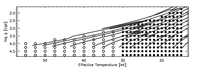
Figure 1: Selected Bstar2006  grid points (full) and Ostar2002 grid points (open) in the $\log g\ vs.$ $T_{\rm eff}$  plan. The two grids overlap at $T_{\rm eff}$= 30 000 K. Geneva evolutionary tracks (Schaller et al., 1992) are shown for solar metallicity, and correspond to models with initial masses of 120, 85, 60, 40, 25, 20, 15, 12, 9, 7, 5, and 4 $M_{\sun}$ from left to right, respectively.

For each of the five metallicities, we have thus computed 265 model atmospheres. This includes a full set of 163 models at the lower microturbulence, and two sets of 51 models at the higher microturbulence (include only low gravity models). At the highest metallicities, a few models very close to the Eddington limit could not be converged because of physical and numerical instabilities; these few models are thus skipped. Fig. 1 illustrates the sampling of the $\log g$ vs. $T_{\rm eff}$  diagram by our two grids of NLTE model atmospheres. The two grids overlap at $T_{\rm eff}$ = 30 000 K, and we show below a comparison.

4.1 Output Products and Availability

The model atmospheres are available at the TLUSTY Web site. Similarly to the Ostar2002 grid, each model is characterized by a unique filename describing the parameters of the model, for example BS25000g275v10CN. The first letters indicate the composition, followed by the effective temperature, the gravity and the turbulent velocity. For models with altered surface composition (supplemental set 2), “CN” is appended to the filename. We have adopted the same key for the models’ overall composition as in the Ostar2002 grid (see Table 2), that is: twice solar (“BC models”), solar (“BG models”), half solar (“BL models”), one fifth solar (“BS models”), one tenth solar (“BT models”), and metal-free (“BZ models”). Model atmospheres with even lower metallicities as in the Ostar2002 grid may be made available at a future time.

Each model comes as a set of six files, with an identical filename’s root but a different extension. A complete description of the files’ content and format can be found in TLUSTY User’s guide (see TLUSTY web site); for reference, we describe them only very briefly here:
model.5: General input data;
model.nst: Optional keywords;
model.7: Model atmosphere: Temperature, electron density, total density and NLTE populations as function of depth;
model.11: Model atmosphere summary;
model.12: Model atmosphere: Similar to model.7, but NLTE populations are replaced by NLTE $b$-factors (LTE departure coefficients);
model.flux: Model flux distribution from the soft X-ray to the far-infrared given as the Eddington flux $H_{\nu}$ [in erg s^-1 cm^-2 Hz^-1] as function of frequency.

The model fluxes are provided at all frequency points included in the calculations (about 380 000 points with an irregular sampling for the low microturbulence models; about 175 000 points for the “v10” models). Additionally, we have calculated detailed emergent spectra with SYNSPEC, version 48, in the ultraviolet ($\lambda\lambda$900-3200 Å) and in the optical ($\lambda\lambda$3200-10 000 Å). Filename extensions are model.uv.7, model.vis.7, respectively, and *.17 for the continuum spectra. Additional spectra in other wavelength ranges, with altered chemical compositions, or with different values of the microturbulent velocity can be readily computed using SYNSPEC. The spectrum synthesis requires three input files, model.5, model.7, and model.nst, and the necessary atomic data files (model atoms and the relevant linelist).

The analysis of individual stars may require to interpolate within the model grid. Interpolation procedures were discussed in Paper I, §5.2. Since the Bstar2006  grid is sampled with a temperature step (1000 K) that is even finer than the step in the Ostar2002 grid, these procedures can be applied. As the safest method, however, we advise to interpolate the atmospheric structure for the selected parameters, followed by recalculating the spectrum with SYNSPEC. This approach provides a very fast way to apply these fully-blanketed NLTE model atmospheres to detailed spectrum analyses of B stars.

4.2 Model Sensitivity

We have investigated the effect of several assumptions made to calculate the Bstar2006 model atmospheres, including the treatment of iron opacity, the choice of the “standard” solar abundances, and the adopted model atoms. For these tests, we have selected the solar composition model, $T_{\rm eff}$= 25 000 K, $\log g~{}=~{}4.0$, $V_{\rm t}$ = 2 km s^-1, and one solar composition model ($T_{\rm eff}$= 30 000 K, $\log g~{}=~{}3.0$) where the two grids overlap.

The first test expands at lower $T_{\rm eff}$  on the tests of iron line-blanketing made in Paper I, §8. Based on earlier experience and mostly on the importance of representing blends as accurately as possible, we preferentially adopt Opacity Sampling (OS) over the Opacity Distribution Function approach. In order to ensure the best description of line blends, we have used a small frequency sampling step (0.75 fiducial Doppler width) as the standard. We have then tested the resulting effect on the atmospheric structure of a larger sampling step and of a different line strength selection criterion. Compared to the reference solar composition model BG25000g400v2, model BG25a uses a frequency sampling step that is 40 times larger for the iron lines, without any changes for lines of lighter species, hence reducing the total number of frequencies by a factor of about 3. Model BG25b limits the dynamically selected iron lines to the strongest lines, selecting about 85,000 lines of Fe II to Fe V compared to over 1,500,000 lines in the reference model. Fig. 2 (left panel) displays the change in the atmospheric temperature structure with repect to the reference model. The temperature differences remain small, quite comparable to the changes seen in similar tests for O star model atmospheres. As a reference, the typical numerical accuracy achieved in conserving the total radiative flux corresponds to uncertainties up to 10 – 20 K on the local temperature. The limited extent of temperature changes found in these tests implies only minimal changes in the predicted spectra, as exemplified by the test with different standard abundances where the temperature changes are somewhat larger (see below, and Figs. 2 and 3). We believe that the tests that we performed for O and B star model atmospheres are representative to the numerical accuracy of Opacity Sampling in hot model atmospheres. The larger sampling step might thus be quite sufficient for most purposes, hence allowing a substantial saving in computer time (up to a factor of 3). However, because we intend the Bstar2006  grid to serve as reference NLTE model atmospheres, and since accuracy testing is practicable only in a limited extent, we have elected to keep the finest sampling to ensure the best description of iron line blanketing.

When we initiated the work on the Ostar2002 and Bstar2006  grids, we adopted the standard solar abundances from Grevesse & Sauval (1998). In the interim, several studies showed that the carbon, nitrogen, and oxygen abundances in the Sun are significantly lower, about 70% of the earlier standard values (Asplund et al., 2005). The new lower abundances are in good agreement with abundances measured in B stars in the solar neighborhood (e. g., Cunha & Lambert, 1994). Additionally, Cunha et al. (2006) found that the neon abundance in the Orion B stars is twice the standard value, and they argued that this value might be used as a good proxy for the solar abundance. Accordingly, we investigated the differences in atmospheric structure and predicted spectrum from these updated C, N, O, and Ne abundances, calculating a model atmosphere using $T_{\rm eff}$ = 25 000 K, $\log g=4.0$, $V_{\rm t}$ = 2 km s^-1, and the newer abundances. For the comparison, we considered 4 different model atmospheres: two models in the grid for solar (BG25) and half-solar (BL25) metallicities (since the new CNO values fall in between), the BGA25 model atmosphere with the new abundances, and a model spectrum BGZ25 calculated with the solar composition atmospheric structure and applying the new abundances in the spectrum calculation step only. Fig. 2 (right panel) shows the temperature differences between the first three models. The changes resulting from the changes in the light element abundances remain limited ($\Delta T~{}<~{}90$ K), and they are as much as 4 times smaller than the differences between the solar and half-solar metallicity models. This comparison shows the importance of iron line blanketing in establishing the temperature structure. We then compare the resulting effect of the abundance changes on the predicted spectra. We show in Fig. 3 the spectral region around H$\gamma$, also including He I $\lambda$4388 and many O II lines, and the relative differences between the model spectra. The absolute continuum flux level changes by less than 1%, and up to 2% for the half-solar metallicity model. The largest changes, 4% and higher, are seen in line cores, mostly in the strength of O II lines which are directly related to changes in the oxygen abundance in the spectrum calculation. Most importantly, however, the BGZ25 model spectrum is very similar to the BGA25 model spectrum (see Fig. 3, middle panel of 3 showing the relative changes) and, therefore, shows that the largest spectrum changes directly result indeed from abundance changes in the spectrum synthesis step rather than from the indirect change in the atmospheric structure. In most cases, it might therefore be appropriate to use the solar composition model atmospheres and only to recalculate the spectra with the updated abundances of light species. We finally stress that the highest accuracy will always be reached when tailoring the model atmospheres to the stars studied, using the closest estimates of all stellar parameters and abundances; the Bstar2006  grid primarily intends to provide the best starting point for these detailed analyses.

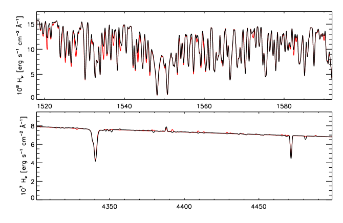
Figure 4: Ultraviolet and visible model spectra for model atmospheres with identical stellar parameters ($T_{\rm eff}$ = 30 000 K, $\log g=3.0$, solar composition, and $V_{\rm t}$ = 10 km s^-1) from the two grids: Bstar2006  (black line) and Ostar2002 (grey line, red line in electronic edition). A rotational broadening of 50 km s^-1  was applied to the spectra.

Finally, we examine the sensitivity of model stellar atmospheres to the adopted model atoms by comparing a model atmosphere with identical parameters ($T_{\rm eff}$ = 30 000 K, $\log g=3.0$, solar composition, and $V_{\rm t}$ = 10 km s^-1) from the two grids, Bstar2006 and Ostar2002. Sect. 3 details the atom models and changes between the two grids. In summary, the newer models includes lower ionization ions as well as more complete model atoms, in particular for C III, N II, N IV, O II, O III, and the Ne and S ions. Fig. 4 illustrates the very high consistency between the two grids: the very rich ultraviolet and the visible spectra predicted by these two calculations are very much the same. Rotational broadening ($V\sin i~{}=~{}50$ km s^-1) has been applied to the spectra to show a comparison that is more relevant to actual spectral analyses. In the visible spectrum, we particularly note on one hand the excellent agreement in H$\gamma$, He I $\lambda$4471, and He I $\lambda$4388 in emission, while weak metal lines on the other hand reveal some discrepancies. A closer examination shows that Balmer lines are predicted very slightly weaker in the Bstar2006  models than in the Ostar2002 models, which we interpret as resulting from the adoption of different bound-bound collisional rates in hydrogen. This small difference has an insignificant impact on the derived stellar parameters. All metal lines showing changes in the optical spectrum arise from highly-excited levels. Hence, these differences are likely a consequence of the newer model atoms that explicitly include higher levels in the NLTE calculations. The $gf$-values of some lines in the linelist used by SYNSPEC have also been updated from the original Kurucz data to OP data for consistency between the model atmosphere and the spectrum synthesis calculations. We expect the OP values to be of higher accuracy in general. From this last test, we may therefore conclude that the two model atmosphere grids will yield consistent results. Although these models include a detailed and extensive treatment of line blanketing, we stress that these models should not be applied blindly to the analysis of some weak lines in the visible and infrared range without a line-by-line assessment of the adequacy of the model atoms in each case.

5 REPRESENTATIVE RESULTS

In this section, we show some basic properties and important trends describing model atmospheres of B-type stars, in particular a comparison to Kurucz (1993) LTE model atmospheres and spectra, ionization structure, bolometric corrections, and radiative accelerations.

5.1 Comparison to LTE Model Atmospheres

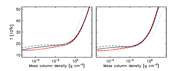
Figure 5: Temperature structure of model atmospheres with $T_{\rm eff}$= 25 000 K, $\log g=3.0$ (left panel) and $\log g=4.0$ (right panel). Black lines show the temperature stratification of the NLTE BSTAR2006 models, compared to the LTE Kurucz models (grey lines; red in electronic edition). Solar composition models (full lines) and metal-poor (1/10 solar) models (dashed lines) are displayed. The dotted lines illustrate the effect of the different surface gravities.

We first compare the atmospheric structure of NLTE Bstar2006  and LTE Kurucz (1993) model atmospheres. Figure 5 displays the temperature stratification of a series of solar composition and one-tenth solar metallicity NLTE and LTE models, $T_{\rm eff}$ = 25 000 K, $\log g~{}=$ 3.0 and 4.0. At large depths ($\tau_{\rm Ross}\gtrsim 1$, corresponding to mass column densities larger than 0.5 g cm^-2) where the departures from LTE are small, the LTE and NLTE atmospheric temperature structures are very similar. This agreement thus provides good support to the two independent approaches (Kurucz ODFs and our OS treatment) to incorporate the opacity of millions of lines in model stellar atmospheres. In shallower layers, the local temperature in NLTE models is higher than in the LTE models. In the NLTE models, temperature is basically determined by a balance between heating by the Balmer hydrogen lines and cooling by lines of heavy elements (carbon and heavier elements). Figure 5 illustrates that the classical NLTE temperature rise is not completely removed by the cooling from metal lines, even at solar metallicity, and shows the metallicity dependence of this effect. We may therefore expect from this comparison that LTE and NLTE continuum spectra will not differ too much, while the core of strong lines and lines from minor ions will be most affected by departures from LTE.

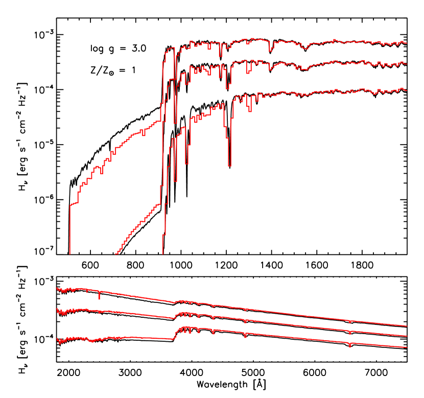
Figure 6: Predicted flux for three solar composition model atmospheres with $(T_{\rm eff},\log g)$ equal to (25000 K, 3.0); (20000 K, 3.0), and (15000 K, 3.0) – black lines; compared to Kurucz (1993) models with the same parameters – grey histograms (red in electronic edition).

We then compare the predicted spectra of our NLTE line-blanketed model atmospheres with Kurucz (1993) LTE model spectra. Fig. 6 displays a comparison of the predicted LTE and NLTE spectral energy distributions for 3 solar composition models with $\log g=3.0$ and $V_{\rm t}$ = 2 km s^-1. For this comparison, we use the spectra directly calculated by TLUSTY (files model.flux described earlier), but not detailed spectra computed by SYNSPEC. For clarity, the spectra are smoothed over 800 frequency points; this roughly simulates the 10 Å resolution of Kurucz (1993) model spectra. This figure reveals some differences in the continuum fluxes, most noticeably in the near ultraviolet where the LTE fluxes are about 10% higher than the NLTE predictions. The lower NLTE fluxes result from the overpopulation of the H I $n=2$ level at the depth of formation of the continuum flux, hence implying a larger Balmer continuum opacity. A smaller difference is seen in the Paschen continuum of the cooler models because of overpopulation of the $n=3$ level. At higher surface gravities, these differences are still present albeit reduced. To conserve the total flux, the LTE models show a lower flux in the far and extreme ultraviolet. In the hottest model shown ($T_{\rm eff}$ = 25 000 K), the LTE prediction in the Lyman continuum in a factor of 2 lower than the NLTE flux. In the cooler models, the LTE flux is lower at wavelengths shorter than Ly $\alpha$.

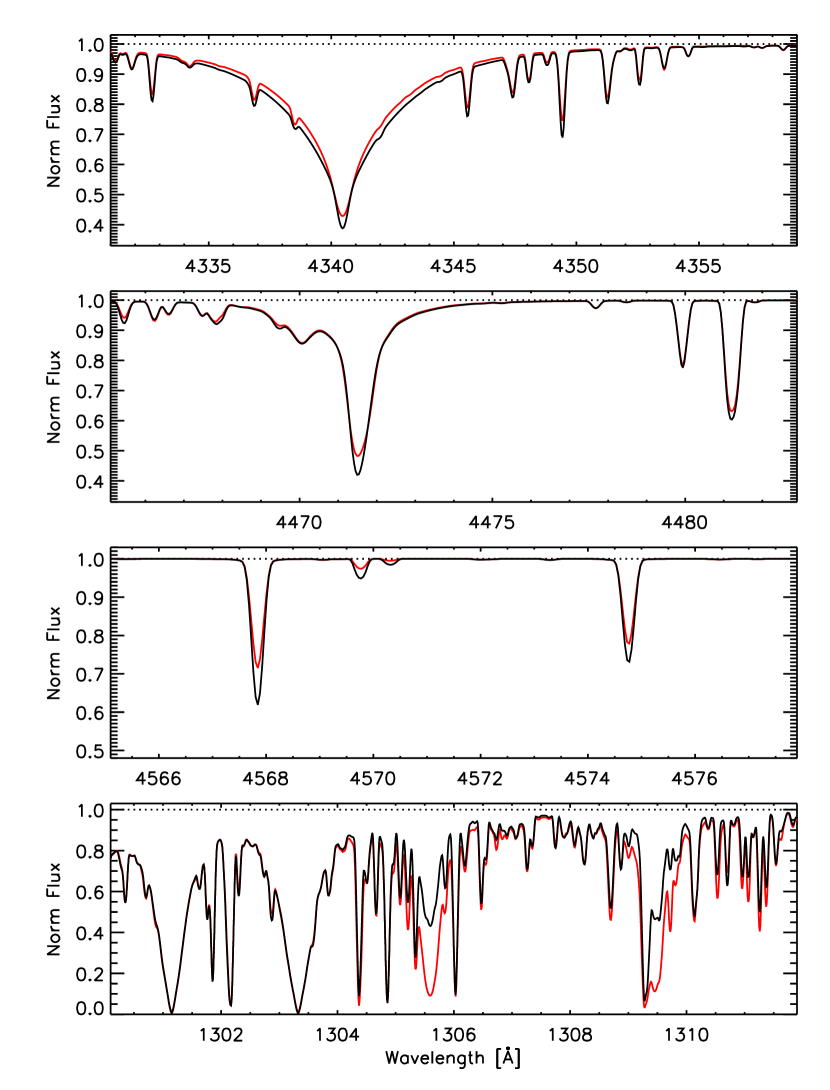
Figure 7: Predicted line profiles for a solar composition model atmospheres with $T_{\rm eff}$ = 20 000 K, $\log g=3.0$, and $V_{\rm t}$ = 2 km s^-1 – black lines; compared to the Kurucz (1993) model with the same parameters – grey lines (red lines in electronic edition).

In the last step comparing the Bstar2006  models to LTE models, we examine detailed line profiles calculated with SYNSPEC, using either a TLUSTY model atmosphere or a Kurucz model atmosphere ($T_{\rm eff}$ = 20 000 K, $\log g=3.0$, solar composition, and $V_{\rm t}$ = 2 km s^-1). We have convolved the spectra with a rotation broadening (10 km s^-1) and normalized the spectra to the continuum. To compute the spectra, we have used the same atomic line list, hence all differences result from level populations departing from the LTE value or differences in the atmospheric model structure. Some typical behaviors are illustrated in Fig. 7. In the NLTE model, the hydrogen Balmer lines are broader and stronger. For the main part, this is the result of the overpopulation of the $n=2$ level. Stellar analyses relying on LTE model atmospheres therefore tend to overestimate surface gravities derived from Balmer line wings. Other optical lines differ little (e. g., O II lines, or Al III $\lambda$4480) or are somewhat stronger in the NLTE model spectrum (e. g., He I $\lambda$4471, Mg II $\lambda$4481, or Si III $\lambda\lambda$4552, 4567, 4575). In the latter case, this implies that the abundance of some species might be overestimated from LTE predictions; for instance, a LTE analysis of Ne I lines overestimates the neon abundance up to 0.5 dex (Cunha et al., 2006). Finally, Fig. 7 shows a comparison in the far ultraviolet around 1300 Å, illustrating the effect of NLTE radiative overionization. Lines of the dominant ions, such as Si III $\lambda\lambda$1301, 1303, remain virtually unchanged, while lines of minor ions (e. g., Si II $\lambda\lambda$1305, 1309) are significantly weaker in the NLTE model. The weak Si II lines mainly result from the typical radiative overionization found in NLTE models; differences in atmospheric structure have a limited influence. While using Kurucz LTE models might have been a reasonable choice for analyzing UV and optical spectra of B-type stars, these comparisons demonstrate that the new Bstar2006  NLTE line-blanketed model atmospheres represent a significant progress for determining the stellar parameters and the surface chemical composition of these stars. We plan to present a systematic study of various effects and differences between LTE and NLTE models, and their influence on deduced stellar parameters, in a future paper.

5.2 Ionization Fractions

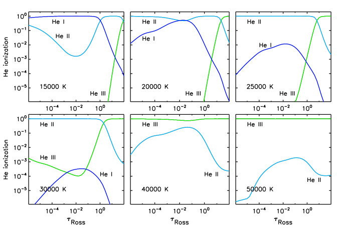
Figure 8: Ionization fractions of helium as function of depth in 6 NLTE model atmospheres, $T_{\rm eff}$= 15 000, 20 000, 25 000, 30 000, 40 000 and 50 000 K, $\log g=4.0$, and solar composition.

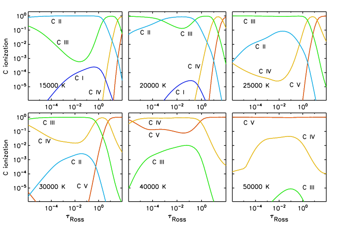
Figure 9: Ionization fractions of carbon as function of depth in 6 NLTE model atmospheres, $T_{\rm eff}$= 15 000, 20 000, 25 000, 30 000, 40 000 and 50 000 K, $\log g=4.0$, and solar composition.

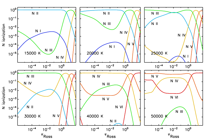
Figure 10: Ionization fractions of nitrogen as function of depth in 6 NLTE model atmospheres, $T_{\rm eff}$= 15 000, 20 000, 25 000, 30 000, 40 000 and 50 000 K, $\log g=4.0$, and solar composition.

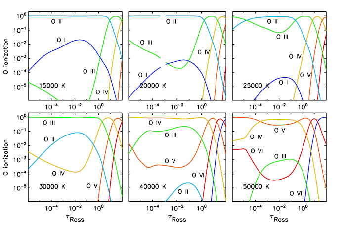
Figure 11: Ionization fractions of oxygen as function of depth in 6 NLTE model atmospheres, $T_{\rm eff}$= 15 000, 20 000, 25 000, 30 000, 40 000 and 50 000 K, $\log g=4.0$, and solar composition.

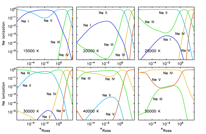
Figure 12: Ionization fractions of neon as function of depth in 6 NLTE model atmospheres, $T_{\rm eff}$= 15 000, 20 000, 25 000, 30 000, 40 000 and 50 000 K, $\log g=4.0$, and solar composition.

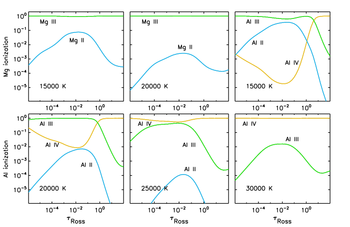
Figure 13: Ionization fractions of magnesium and aluminum as function of depth in 4 NLTE model atmospheres, $T_{\rm eff}$= 15 000, 20 000, 25 000, and 30 000 K, $\log g=4.0$, and solar composition.

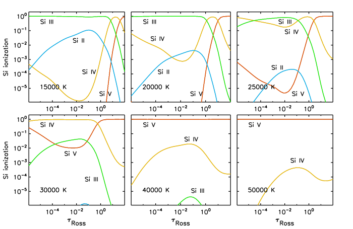
Figure 14: Ionization fractions of silicon as function of depth in 6 NLTE model atmospheres, $T_{\rm eff}$= 15 000, 20 000, 25 000, 30 000, 40 000 and 50 000 K, $\log g=4.0$, and solar composition.

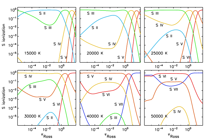
Figure 15: Ionization fractions of sulfur as function of depth in 6 NLTE model atmospheres, $T_{\rm eff}$= 15 000, 20 000, 25 000, 30 000, 40 000 and 50 000 K, $\log g=4.0$, and solar composition.

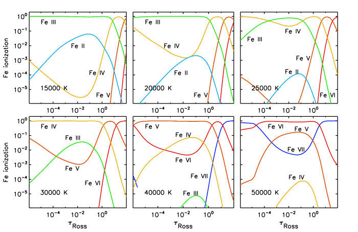
Figure 16: Ionization fractions of iron as function of depth in 6 NLTE model atmospheres, $T_{\rm eff}$= 15 000, 20 000, 25 000, 30 000, 40 000 and 50 000 K, $\log g=4.0$, and solar composition.

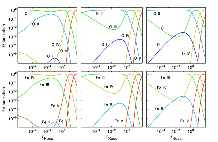
Figure 17: Ionization fractions of oxygen and iron as function of depth in 3 NLTE model atmospheres with different surface gravities ($\log g=2.25,3.25,4.25$, from left to right). Solar composition and $T_{\rm eff}$= 20 000 K is assumed for the 3 models.

Figures 8–16 display the ionization fractions of all explicit species (with the exception of hydrogen) in model atmospheres spanning the range of temperature of the Bstar2006  grid. For completion, we have added two hotter O star model atmospheres ($T_{\rm eff}$ = 40,000 K and 50,000 K), thus providing a comprehensive view of the change in ionization from 15 000 K to 50 000 K. We show the ionization structure of solar composition, main-sequence ($\log g=4.0$) star atmospheres. The 6 selected model atmospheres roughly correspond to spectral types B5, B2.5, B1, B0, O5, and O2-O3. These figures thus give a straightforward illustration of the change in the expected line strength for various ions along the spectral type sequence, and support our choice of explicit NLTE ions. At depth ($\tau_{\rm Ross}\gtrsim 10$), the ionization fractions may become incorrect when higher ions have been neglected, most particularly for magnesium and aluminum. We stress however that this restriction does not affect the predicted spectra at all. Fig. 17 compares the oxygen and iron ionization in model atmospheres with increasing surface gravities. At $T_{\rm eff}$ = 20 000 K, the ionization shifts up by one degree between a main-sequence model ($\log g=4.25$) and a supergiant model ($\log g=2.25$). Higher ionization at lower gravities is a well-known result, which follows from the Saha formula and from the typical NLTE radiative overionization. Finally, a comparison of the ionization structure of models with low and high microturbulent velocities shows that ionization is very slightly higher in models with the higher microturbulence. There is virtually no change in the dominant ion; with respect to this ion, lower ions are less populated and higher ions are more populated in models with the higher microturbulence. We interpret this change as a consequence of the stronger line blanketing. The enhanced line blocking results in slightly higher temperature at depth because of backwarming. The ions are thus exposed to a harder radiation field, hence the slight ionization shift.

These ionization fractions are useful to roughly assess the expected strengths of individual spectral lines. However, the ionization fractions should not be taken too literally. In some important cases, lines may originate from very high-lying levels whose populations may be a tiny fraction of the total abundance of a specific ion. In those cases, relying on the ionization fractions displayed in Figs 8–16 alone may be misleading. The interested reader may however always access the individual level populations that are stored in files model.7, as well as the individual NLTE departure coefficients stored in files model.12 to estimate better the expected line strengths, or the ratios of line strengths for lines of different ions of the same species.

5.3 Bolometric Corrections and Ionizing Fluxes

Bolometric corrections (Table 3) are calculated using the following expression:

$$BC_{V}=m_{\rm bol}-V=(-2.5\log F_{\rm bol}-11.487)-(-2.5\log F_{V}-21.100)$$ (1)

where $F_{\rm bol}$ is the bolometric flux and $F_{V}$ is the flux through the Johnson $V$ filter, computed from the model atmospheres’ flux distribution. The bolometric flux is computed by trapezoidal integration over the complete frequency range, while we have used an IDL version of the program ubvbuser (Kurucz, 1993) kindly made available by Wayne Landsman to obtain the $V$ magnitudes. The first constant is defined by assuming a solar value, $BC_{V}^{\sun}=-0.07$, while the second constant defines the zero point of the $V$ magnitude scale.

Fig. 18 illustrates the major dependence of the bolometric correction with the effective temperature (solar metallicity, $\log g=4.0$). We have extended the plot to encompass both the Bstar2006  and the Ostar2002 models. Dependences in terms of the other stellar parameters (gravity, metallicity and microturbulent velocity) are much weaker than the temperature dependence. While we find differences up to 0.1 mag over the whole range in metallicity (twice solar to metal-free), the changes remain limited to a few hundredths of a magnitude for different gravities and microturbulences. Larger differences are found for models very close to the Eddington limit, but these models are in a domain where our basic assumption of static atmospheres starts to break up. The small step (0.05 dex) in the overlapping range between the two grids is therefore most likely a consequence of the differences in the treatment of opacities, that is, it likely results from the different ions, levels and lines explicitly included in the model atmospheres. The bolometric corrections of “CN” models do not differ from models with unaltered compositions, and they are thus not listed in Table 3.

Ionizing photons are emitted essentially by hot, massive stars, and the extreme ultraviolet flux drops precipitously in early B stars with diminishing effective temperatures. Therefore, we only provide in Table 4 a summarized extension of the Ostar2002 Lyman continuum fluxes to the early B star domain.

5.4 Radiative Acceleration and Effective gravities

The comprehensive treatment of opacities in the Bstar2006  model atmospheres allows for an accurate estimate of radiative pressure on the atmospheric structure. TLUSTY thus provides a run of radiative acceleration with depth, see Fig. 2 in Paper I for an illustration. In every model atmosphere, the radiative acceleration goes through a local maximum in the continuum forming region ($\tau_{\rm Ross}\approx 1$), and then shows another strong increase in very superficial layers ($\tau_{\rm Ross}\lesssim 10^{-6}$). In low gravity models, the radiative acceleration may exceed gravity at these depths indicating that the top layers are unstable. The assumption of hydrostatic equilibrium then break down there. We have numerically limited the radiative acceleration in these superficial layers to ensure convergence following the prescription used in Paper I. The model spectra are not affected by this approximation, because these superficial layers only influence the strong resonance lines that form in a stellar wind. The photosperic stability is more appropriately defined by the maximum reached by the radiative acceleration around optical depth unity (see Fig. 2, Paper I). Fig. 19 displays isocontours of this maximum relative to the gravitational acceleration, $\Gamma_{\rm rad}=\max(g_{\rm rad})/g$, as a function of effective temperature and gravity. Models tend to become numerically unstable when $\Gamma_{\rm rad}>0.9$, setting thus the gravity limit in our grid.

We can extrapolate these radiative acceleration to define the limit of photospheric stability when $\Gamma_{\rm rad}$ reaches unity, thus providing with an estimate of the Eddington limit in absence of rotation (see Fig. 19). Table 5 gives $\log g_{\rm Edd}$, the Eddington limit in term of $\log g$, as a function of effective temperature from 55 000 to 15 000 K. We have carried out the same extrapolation with metal-free model atmospheres, and found that the corresponding Eddington limit is reached about 0.05 dex lower than the values derived for solar composition models. Lamers & Fitzpatrick (1988) performed a similar exercise, defining the Eddington limit by extrapolating the radiative accelerations calculated with Kurucz model atmospheres. Their estimates agree very well with our results over the whole range of temperature.

Finally, we can derive effective gravities, $g_{\rm eff}=g-\max(g_{\rm rad})$, in absence of rotation (see Table 5). These effective gravities may be used to estimate the characteristic pressure scale height ($h=P_{\rm gas}/g_{\rm eff}$) in the photosphere, after possibly correcting $g_{\rm eff}$ further for centrifugal acceleration. These scale heights indicate that the photosphere of main-sequence B stars are compact with scale heights typically smaller than 1% of the stellar radius. On the other hand, the photosphere of extreme B supergiants ($\log g\leq 2.0$) are quite extended ($h>1R_{\sun}$, or several percent of their radius). Caution should be exercised when applying these model atmospheres to analyze the spectra of these supergiants.

6 CONCLUSION

We have constructed a comprehensive grid of metal line-blanketed, NLTE, plane-parallel, hydrostatic model atmospheres for the basic parameters appropriate to early B-type stars. The Bstar2006  grid considers 16 values of effective temperatures 15 000 K $\leq$$T_{\rm eff}$ $\leq$ 30 000 K, with 1 000 K steps, 13 surface gravities, $1.75\leq\log g\leq 4.75$ with 0.25 dex steps, and 6 chemical compositions, from metal-rich relative to the Sun to metal-free. The lower limit of $\log g$ for a given $T_{\rm eff}$  is actually set by an approximate location of the Eddington limit. The complete Bstar2006  grid is available at our website at http://nova.astro.umd.edu.

We have intended to provide a more or less definitive grid of model atmospheres in the context of one-dimensional, plane-parallel, homogeneous, hydrostatic models in radiative equilibrium. We have attempted to take into account essentially all important opacity sources (lines and continua) of all astrophysically important ions. Likewise, we have attempted to consider all relevant atomic processes that determine the excitation and ionization balance of all such atoms and ions. The models explicitly include, and allow for departures from LTE, 46 ions of H, He, C, N, O, Ne, Mg, Al, Si, S, and Fe, and about 53 000 individual atomic levels (including about 49 300 iron levels) grouped into 1127 superlevels. Line opacity includes about 39 000 lines from the light elements and 500 000 to 2 million iron lines dynamically selected from a list of about 5.65 million lines.

Although we spent all effort to make sure that the treatment of atomic physics and opacities is as complete and accurate as possible, there are still several points we are aware of that were crudely approximated. Those approximations were necessitated not by shortcomings of our modeling scheme or a lack of adequate computer resources, but by the present lack of sufficient atomic data. These approximations include a crude and approximate treatment of collision rates, a neglect of very high energy levels of light metals, and ignoring charge exchange reactions. Despite our updating most model atoms to include levels up to $n=10$, we caution that the analysis of weak lines from highly excited energy levels in the optical and infrared spectrum might require to construct even more detailed model atoms, supplementing the model atoms with higher excitation levels, or possibly also splitting some superlevels into individual levels.

Despite the remaining approximations and uncertainties, we believe that the Bstar2006  grid represents a definite improvement over previous grids of B star model atmospheres. Combined with our earlier Ostar2002 grid of O star model atmospheres, we hope that these new model atmospheres will thus be useful for a number of years to come for analyzing the spectrum individual O and B stars, as well as constructing composite model spectra of clusters of young massive stars, OB associations, and starburst galaxies.

Table 1: Atomic data included in the NLTE model atmospheres.

Ion	(Super)Levels	Indiv. Levels	Lines	References
H I	9string	80string	172string
H II	1string	1string	$\cdots$
He I	24string	72string	784string	1
He II	20string	20string	190string
He III	1string	1string	$\cdots$
C I	40string	239string	3201string	2
C II	22string	44string	238string	3
C III	46string	95string	738string	4
C IV	25string	55string	330string	5
C V	1string	1string	$\cdots$
N I	34string	115string	785string	6
N II	42string	247string	3396string	2
N III	32string	68string	549string	3
N IV	48string	126string	1093string	4
N V	16string	55string	330string	5
N VI	1string	1string	$\cdots$
O I	33string	69string	418string	7
O II	48string	218string	3484string	6
O III	41string	267string	3855string	2
O IV	39string	94string	922string	3
O V	6string	6string	4string	4
O VI	1string	1string	$\cdots$
Ne I	35string	191string	2715string	8
Ne II	32string	167string	2301string	7
Ne III	34string	149string	1354string	7
Ne IV	12string	18string	38string	6
Ne V	1string	1string	$\cdots$
Mg II	25string	53string	306string	9
Mg III	1string	1string	$\cdots$
Al II	29string	81string	536string	10
Al III	23string	53string	306string	9
Al IV	1string	1string	$\cdots$
Si II	40string	64string	392string	11
Si III	30string	105string	747string	10
Si IV	23string	53string	306string	9
Si V	1string	1string	$\cdots$
S II	33string	226string	4166string	13
S III	41string	235string	3452string	12
S IV	38string	100string	909string	11
S V	25string	131string	1171string	10
S VI	1string	1string	$\cdots$
Fe II	36string	10 921string	1 264 969string	14, 15
Fe III	50string	12 660string	1 604 934string	14, 16
Fe IV	43string	13 705string	1 776 984string	14, 17
Fe V	42string	11 986string	1 008 385string	14, 18
Fe VI	1string	1string	$\cdots$

References. — (1) http://physics.nist.gov/PhysRefData/ASD/index.html; (2) Luo & Pradhan 1989; (3) Fernley et al. 1999; (4) Tully, Seaton, & Berrington 1990; (5) Peach, Saraph, & Seaton 1988; (6) V. M. Burke & D. J. Lennon, to be published; (7) K. Butler & C. J. Zeippen, to be published; (8) Hibbert & Scott 1994; (9) K. T. Taylor, to be published; (10) Butler, Mendoza, & Zeippen 1993; (11) Mendoza et al. 1995; (12) Nahar & Pradhan 1993; (13) K. Butler, C. Mendoza, & C. J. Zeippen, to be published; (14) Kurucz 1994; (15) Nahar 1997; (16) Nahar 1996; (17) Bautista & Pradhan 1997; (18) Bautista 1996.

Table 2: Key to the models’ chemical compositions.

Key	Metallicity
C	$2\times\sun$
G	$1\times\sun$
L	$1/2\times\sun$
S	$1/5\times\sun$
T	$1/10\times\sun$
Z	$0$

Table 3: Bolometric corrections as function of effective temperature, gravity, microturbulent velocity and metallicity (6 metallicities from 2 times solar to metal-free models).

		BC [mag]
$V_{\rm turb}$		2 km s-1							10 km s-1
$Z/Z_{\sun}$		2.	1.	0.5	0.2	0.1	0.		2.	1.	0.5	0.2	0.1	0.
$T_{\rm eff}$  [K]	$\log g$
15,000…	1.75	$-$1.29	$-$1.32	$-$1.33	$-$1.35	$-$1.36	$-$1.39		$-$1.26	$-$1.29	$-$1.32	$-$1.34	$-$1.36	$-$1.40
	2.00	$-$1.23	$-$1.26	$-$1.28	$-$1.30	$-$1.31	$-$1.33		$-$1.19	$-$1.23	$-$1.26	$-$1.29	$-$1.30	$-$1.34
	2.25	$-$1.21	$-$1.24	$-$1.26	$-$1.28	$-$1.29	$-$1.31		$-$1.17	$-$1.21	$-$1.24	$-$1.27	$-$1.28	$-$1.32
	2.50	$-$1.20	$-$1.23	$-$1.26	$-$1.28	$-$1.29	$-$1.30		$-$1.16	$-$1.20	$-$1.23	$-$1.26	$-$1.28	$-$1.31
	2.75	$-$1.20	$-$1.23	$-$1.25	$-$1.27	$-$1.28	$-$1.30		$-$1.16	$-$1.20	$-$1.23	$-$1.26	$-$1.27	$-$1.30
	3.00	$-$1.20	$-$1.23	$-$1.25	$-$1.27	$-$1.28	$-$1.30		$-$1.15	$-$1.20	$-$1.23	$-$1.26	$-$1.27	$-$1.30
	3.25	$-$1.20	$-$1.23	$-$1.25	$-$1.27	$-$1.28	$-$1.30		$\cdots$	$\cdots$	$\cdots$	$\cdots$	$\cdots$	$\cdots$
	3.50	$-$1.19	$-$1.23	$-$1.25	$-$1.27	$-$1.28	$-$1.30		$\cdots$	$\cdots$	$\cdots$	$\cdots$	$\cdots$	$\cdots$
	3.75	$-$1.19	$-$1.22	$-$1.25	$-$1.27	$-$1.28	$-$1.29		$\cdots$	$\cdots$	$\cdots$	$\cdots$	$\cdots$	$\cdots$
	4.00	$-$1.19	$-$1.22	$-$1.25	$-$1.27	$-$1.28	$-$1.29		$\cdots$	$\cdots$	$\cdots$	$\cdots$	$\cdots$	$\cdots$
	4.25	$-$1.19	$-$1.22	$-$1.24	$-$1.26	$-$1.27	$-$1.29		$\cdots$	$\cdots$	$\cdots$	$\cdots$	$\cdots$	$\cdots$
	4.50	$-$1.19	$-$1.22	$-$1.24	$-$1.26	$-$1.27	$-$1.29		$\cdots$	$\cdots$	$\cdots$	$\cdots$	$\cdots$	$\cdots$
	4.75	$-$1.19	$-$1.22	$-$1.24	$-$1.26	$-$1.27	$-$1.29		$\cdots$	$\cdots$	$\cdots$	$\cdots$	$\cdots$	$\cdots$
16,000…	2.00	$-$1.39	$-$1.42	$-$1.44	$-$1.46	$-$1.47	$-$1.50		$-$1.34	$-$1.38	$-$1.41	$-$1.44	$-$1.46	$-$1.50
	2.25	$-$1.37	$-$1.40	$-$1.42	$-$1.44	$-$1.45	$-$1.47		$-$1.32	$-$1.36	$-$1.39	$-$1.42	$-$1.44	$-$1.48
	2.50	$-$1.36	$-$1.39	$-$1.41	$-$1.43	$-$1.44	$-$1.46		$-$1.31	$-$1.35	$-$1.39	$-$1.42	$-$1.43	$-$1.47
	2.75	$-$1.36	$-$1.39	$-$1.41	$-$1.43	$-$1.44	$-$1.46		$-$1.31	$-$1.35	$-$1.39	$-$1.42	$-$1.43	$-$1.46
	3.00	$-$1.36	$-$1.39	$-$1.41	$-$1.43	$-$1.44	$-$1.46		$-$1.31	$-$1.36	$-$1.39	$-$1.42	$-$1.43	$-$1.46
	3.25	$-$1.36	$-$1.39	$-$1.41	$-$1.43	$-$1.44	$-$1.46		$\cdots$	$\cdots$	$\cdots$	$\cdots$	$\cdots$	$\cdots$
	3.50	$-$1.36	$-$1.39	$-$1.41	$-$1.43	$-$1.44	$-$1.46		$\cdots$	$\cdots$	$\cdots$	$\cdots$	$\cdots$	$\cdots$
	3.75	$-$1.36	$-$1.39	$-$1.41	$-$1.43	$-$1.44	$-$1.46		$\cdots$	$\cdots$	$\cdots$	$\cdots$	$\cdots$	$\cdots$
	4.00	$-$1.36	$-$1.39	$-$1.41	$-$1.43	$-$1.44	$-$1.46		$\cdots$	$\cdots$	$\cdots$	$\cdots$	$\cdots$	$\cdots$
	4.25	$-$1.36	$-$1.39	$-$1.41	$-$1.43	$-$1.44	$-$1.46		$\cdots$	$\cdots$	$\cdots$	$\cdots$	$\cdots$	$\cdots$
	4.50	$-$1.36	$-$1.39	$-$1.41	$-$1.43	$-$1.44	$-$1.45		$\cdots$	$\cdots$	$\cdots$	$\cdots$	$\cdots$	$\cdots$
	4.75	$-$1.35	$-$1.38	$-$1.41	$-$1.43	$-$1.44	$-$1.45		$\cdots$	$\cdots$	$\cdots$	$\cdots$	$\cdots$	$\cdots$
17,000…	2.00	$-$1.54	$-$1.57	$-$1.59	$-$1.61	$-$1.62	$-$1.66		$-$1.51	$-$1.53	$-$1.56	$-$1.59	$-$1.61	$-$1.67
	2.25	$-$1.51	$-$1.54	$-$1.56	$-$1.58	$-$1.59	$-$1.62		$-$1.45	$-$1.49	$-$1.53	$-$1.56	$-$1.58	$-$1.63
	2.50	$-$1.50	$-$1.53	$-$1.56	$-$1.58	$-$1.59	$-$1.61		$-$1.45	$-$1.49	$-$1.52	$-$1.56	$-$1.57	$-$1.61
	2.75	$-$1.50	$-$1.53	$-$1.56	$-$1.58	$-$1.59	$-$1.61		$-$1.45	$-$1.50	$-$1.53	$-$1.56	$-$1.57	$-$1.61
	3.00	$-$1.51	$-$1.54	$-$1.56	$-$1.58	$-$1.59	$-$1.61		$-$1.46	$-$1.50	$-$1.53	$-$1.56	$-$1.58	$-$1.61
	3.25	$-$1.51	$-$1.54	$-$1.56	$-$1.58	$-$1.59	$-$1.61		$\cdots$	$\cdots$	$\cdots$	$\cdots$	$\cdots$	$\cdots$
	3.50	$-$1.51	$-$1.54	$-$1.57	$-$1.58	$-$1.59	$-$1.61		$\cdots$	$\cdots$	$\cdots$	$\cdots$	$\cdots$	$\cdots$
	3.75	$-$1.51	$-$1.54	$-$1.57	$-$1.59	$-$1.59	$-$1.61		$\cdots$	$\cdots$	$\cdots$	$\cdots$	$\cdots$	$\cdots$
	4.00	$-$1.52	$-$1.55	$-$1.57	$-$1.59	$-$1.60	$-$1.61		$\cdots$	$\cdots$	$\cdots$	$\cdots$	$\cdots$	$\cdots$
	4.25	$-$1.52	$-$1.55	$-$1.57	$-$1.59	$-$1.60	$-$1.61		$\cdots$	$\cdots$	$\cdots$	$\cdots$	$\cdots$	$\cdots$
	4.50	$-$1.52	$-$1.55	$-$1.57	$-$1.59	$-$1.59	$-$1.61		$\cdots$	$\cdots$	$\cdots$	$\cdots$	$\cdots$	$\cdots$
	4.75	$-$1.51	$-$1.54	$-$1.57	$-$1.58	$-$1.59	$-$1.61		$\cdots$	$\cdots$	$\cdots$	$\cdots$	$\cdots$	$\cdots$
18,000…	2.00	$-$1.72	$-$1.74	$-$1.75	$-$1.77	$-$1.79	$-$1.83		$\cdots$	$\cdots$	$-$1.76	$-$1.78	$-$1.80	$-$1.85
	2.25	$-$1.64	$-$1.67	$-$1.69	$-$1.72	$-$1.73	$-$1.77		$-$1.58	$-$1.62	$-$1.65	$-$1.69	$-$1.71	$-$1.77
	2.50	$-$1.63	$-$1.67	$-$1.69	$-$1.71	$-$1.72	$-$1.75		$-$1.57	$-$1.61	$-$1.65	$-$1.69	$-$1.70	$-$1.76
	2.75	$-$1.64	$-$1.67	$-$1.69	$-$1.71	$-$1.72	$-$1.75		$-$1.58	$-$1.62	$-$1.66	$-$1.69	$-$1.71	$-$1.75
	3.00	$-$1.64	$-$1.68	$-$1.70	$-$1.72	$-$1.73	$-$1.75		$-$1.59	$-$1.63	$-$1.67	$-$1.70	$-$1.71	$-$1.75
	3.25	$-$1.65	$-$1.68	$-$1.70	$-$1.72	$-$1.73	$-$1.75		$\cdots$	$\cdots$	$\cdots$	$\cdots$	$\cdots$	$\cdots$
	3.50	$-$1.65	$-$1.69	$-$1.71	$-$1.73	$-$1.74	$-$1.75		$\cdots$	$\cdots$	$\cdots$	$\cdots$	$\cdots$	$\cdots$
	3.75	$-$1.66	$-$1.69	$-$1.71	$-$1.73	$-$1.74	$-$1.76		$\cdots$	$\cdots$	$\cdots$	$\cdots$	$\cdots$	$\cdots$
	4.00	$-$1.66	$-$1.69	$-$1.71	$-$1.73	$-$1.74	$-$1.76		$\cdots$	$\cdots$	$\cdots$	$\cdots$	$\cdots$	$\cdots$
	4.25	$-$1.66	$-$1.69	$-$1.72	$-$1.73	$-$1.74	$-$1.76		$\cdots$	$\cdots$	$\cdots$	$\cdots$	$\cdots$	$\cdots$
	4.50	$-$1.66	$-$1.69	$-$1.72	$-$1.73	$-$1.74	$-$1.76		$\cdots$	$\cdots$	$\cdots$	$\cdots$	$\cdots$	$\cdots$
	4.75	$-$1.66	$-$1.69	$-$1.72	$-$1.73	$-$1.74	$-$1.75		$\cdots$	$\cdots$	$\cdots$	$\cdots$	$\cdots$	$\cdots$
19,000…	2.25	$-$1.77	$-$1.79	$-$1.82	$-$1.84	$-$1.86	$-$1.90		$-$1.73	$-$1.76	$-$1.79	$-$1.82	$-$1.84	$-$1.91
	2.50	$-$1.75	$-$1.79	$-$1.81	$-$1.84	$-$1.85	$-$1.89		$-$1.69	$-$1.73	$-$1.77	$-$1.81	$-$1.83	$-$1.89
	2.75	$-$1.76	$-$1.79	$-$1.82	$-$1.84	$-$1.85	$-$1.88		$-$1.69	$-$1.74	$-$1.78	$-$1.81	$-$1.83	$-$1.88
	3.00	$-$1.77	$-$1.80	$-$1.83	$-$1.85	$-$1.86	$-$1.88		$-$1.71	$-$1.76	$-$1.79	$-$1.82	$-$1.84	$-$1.88
	3.25	$-$1.78	$-$1.81	$-$1.83	$-$1.85	$-$1.86	$-$1.89		$\cdots$	$\cdots$	$\cdots$	$\cdots$	$\cdots$	$\cdots$
	3.50	$-$1.79	$-$1.82	$-$1.84	$-$1.86	$-$1.87	$-$1.89		$\cdots$	$\cdots$	$\cdots$	$\cdots$	$\cdots$	$\cdots$
	3.75	$-$1.79	$-$1.82	$-$1.85	$-$1.86	$-$1.87	$-$1.89		$\cdots$	$\cdots$	$\cdots$	$\cdots$	$\cdots$	$\cdots$
	4.00	$-$1.80	$-$1.83	$-$1.85	$-$1.87	$-$1.88	$-$1.89		$\cdots$	$\cdots$	$\cdots$	$\cdots$	$\cdots$	$\cdots$
	4.25	$-$1.80	$-$1.83	$-$1.85	$-$1.87	$-$1.88	$-$1.89		$\cdots$	$\cdots$	$\cdots$	$\cdots$	$\cdots$	$\cdots$
	4.50	$-$1.80	$-$1.83	$-$1.85	$-$1.87	$-$1.88	$-$1.89		$\cdots$	$\cdots$	$\cdots$	$\cdots$	$\cdots$	$\cdots$
	4.75	$-$1.81	$-$1.83	$-$1.86	$-$1.87	$-$1.88	$-$1.89		$\cdots$	$\cdots$	$\cdots$	$\cdots$	$\cdots$	$\cdots$
20,000…	2.25	$-$1.91	$-$1.93	$-$1.95	$-$1.98	$-$1.99	$-$2.04		$-$1.91	$-$1.92	$-$1.94	$-$1.97	$-$1.99	$-$2.05
	2.50	$-$1.87	$-$1.90	$-$1.93	$-$1.95	$-$1.97	$-$2.01		$-$1.81	$-$1.85	$-$1.88	$-$1.92	$-$1.95	$-$2.01
	2.75	$-$1.87	$-$1.91	$-$1.93	$-$1.96	$-$1.97	$-$2.01		$-$1.80	$-$1.85	$-$1.89	$-$1.93	$-$1.95	$-$2.01
	3.00	$-$1.89	$-$1.92	$-$1.95	$-$1.97	$-$1.98	$-$2.01		$-$1.82	$-$1.87	$-$1.90	$-$1.94	$-$1.96	$-$2.01
	3.25	$-$1.90	$-$1.93	$-$1.96	$-$1.98	$-$1.99	$-$2.01		$\cdots$	$\cdots$	$\cdots$	$\cdots$	$\cdots$	$\cdots$
	3.50	$-$1.91	$-$1.94	$-$1.96	$-$1.98	$-$1.99	$-$2.02		$\cdots$	$\cdots$	$\cdots$	$\cdots$	$\cdots$	$\cdots$
	3.75	$-$1.92	$-$1.95	$-$1.97	$-$1.99	$-$2.00	$-$2.02		$\cdots$	$\cdots$	$\cdots$	$\cdots$	$\cdots$	$\cdots$
	4.00	$-$1.92	$-$1.96	$-$1.97	$-$2.00	$-$2.00	$-$2.02		$\cdots$	$\cdots$	$\cdots$	$\cdots$	$\cdots$	$\cdots$
	4.25	$-$1.93	$-$1.96	$-$1.98	$-$2.00	$-$2.01	$-$2.02		$\cdots$	$\cdots$	$\cdots$	$\cdots$	$\cdots$	$\cdots$
	4.50	$-$1.93	$-$1.96	$-$1.99	$-$2.00	$-$2.01	$-$2.03		$\cdots$	$\cdots$	$\cdots$	$\cdots$	$\cdots$	$\cdots$
	4.75	$-$1.94	$-$1.97	$-$1.99	$-$2.00	$-$2.01	$-$2.02		$\cdots$	$\cdots$	$\cdots$	$\cdots$	$\cdots$	$\cdots$
21,000…	2.25	$\cdots$	$\cdots$	$\cdots$	$-$2.16	$-$2.17	$-$2.22		$\cdots$	$\cdots$	$\cdots$	$-$2.16	$-$2.18	$-$2.23
	2.50	$-$1.98	$-$2.01	$-$2.04	$-$2.06	$-$2.08	$-$2.12		$-$1.94	$-$1.97	$-$2.01	$-$2.04	$-$2.07	$-$2.13
	2.75	$-$1.98	$-$2.01	$-$2.04	$-$2.07	$-$2.09	$-$2.13		$-$1.92	$-$1.96	$-$2.00	$-$2.04	$-$2.06	$-$2.13
	3.00	$-$1.99	$-$2.03	$-$2.06	$-$2.08	$-$2.10	$-$2.13		$-$1.92	$-$1.97	$-$2.01	$-$2.05	$-$2.07	$-$2.13
	3.25	$-$2.01	$-$2.04	$-$2.07	$-$2.09	$-$2.10	$-$2.14		$\cdots$	$\cdots$	$\cdots$	$\cdots$	$\cdots$	$\cdots$
	3.50	$-$2.02	$-$2.06	$-$2.08	$-$2.10	$-$2.11	$-$2.14		$\cdots$	$\cdots$	$\cdots$	$\cdots$	$\cdots$	$\cdots$
	3.75	$-$2.03	$-$2.07	$-$2.09	$-$2.11	$-$2.12	$-$2.14		$\cdots$	$\cdots$	$\cdots$	$\cdots$	$\cdots$	$\cdots$
	4.00	$-$2.04	$-$2.08	$-$2.09	$-$2.12	$-$2.13	$-$2.15		$\cdots$	$\cdots$	$\cdots$	$\cdots$	$\cdots$	$\cdots$
	4.25	$-$2.05	$-$2.08	$-$2.10	$-$2.12	$-$2.13	$-$2.15		$\cdots$	$\cdots$	$\cdots$	$\cdots$	$\cdots$	$\cdots$
	4.50	$-$2.06	$-$2.09	$-$2.11	$-$2.13	$-$2.13	$-$2.15		$\cdots$	$\cdots$	$\cdots$	$\cdots$	$\cdots$	$\cdots$
	4.75	$-$2.06	$-$2.09	$-$2.11	$-$2.13	$-$2.13	$-$2.15		$\cdots$	$\cdots$	$\cdots$	$\cdots$	$\cdots$	$\cdots$
22,000…	2.50	$-$2.10	$-$2.12	$-$2.15	$-$2.18	$-$2.20	$-$2.24		$-$2.07	$-$2.10	$-$2.13	$-$2.17	$-$2.19	$-$2.24
	2.75	$-$2.08	$-$2.12	$-$2.15	$-$2.17	$-$2.19	$-$2.24		$-$2.03	$-$2.07	$-$2.11	$-$2.15	$-$2.17	$-$2.24
	3.00	$-$2.10	$-$2.13	$-$2.16	$-$2.19	$-$2.20	$-$2.24		$-$2.03	$-$2.07	$-$2.11	$-$2.15	$-$2.18	$-$2.24
	3.25	$-$2.11	$-$2.15	$-$2.18	$-$2.20	$-$2.21	$-$2.25		$\cdots$	$\cdots$	$\cdots$	$\cdots$	$\cdots$	$\cdots$
	3.50	$-$2.13	$-$2.16	$-$2.19	$-$2.21	$-$2.22	$-$2.26		$\cdots$	$\cdots$	$\cdots$	$\cdots$	$\cdots$	$\cdots$
	3.75	$-$2.14	$-$2.18	$-$2.20	$-$2.22	$-$2.23	$-$2.26		$\cdots$	$\cdots$	$\cdots$	$\cdots$	$\cdots$	$\cdots$
	4.00	$-$2.15	$-$2.19	$-$2.21	$-$2.23	$-$2.24	$-$2.26		$\cdots$	$\cdots$	$\cdots$	$\cdots$	$\cdots$	$\cdots$
	4.25	$-$2.16	$-$2.19	$-$2.22	$-$2.24	$-$2.25	$-$2.27		$\cdots$	$\cdots$	$\cdots$	$\cdots$	$\cdots$	$\cdots$
	4.50	$-$2.17	$-$2.20	$-$2.22	$-$2.24	$-$2.25	$-$2.27		$\cdots$	$\cdots$	$\cdots$	$\cdots$	$\cdots$	$\cdots$
	4.75	$-$2.18	$-$2.21	$-$2.23	$-$2.24	$-$2.25	$-$2.27		$\cdots$	$\cdots$	$\cdots$	$\cdots$	$\cdots$	$\cdots$
23,000…	2.50	$-$2.24	$-$2.26	$-$2.28	$-$2.31	$-$2.32	$-$2.37		$-$2.25	$-$2.25	$-$2.27	$-$2.30	$-$2.32	$-$2.38
	2.75	$-$2.19	$-$2.22	$-$2.25	$-$2.28	$-$2.29	$-$2.33		$-$2.14	$-$2.18	$-$2.22	$-$2.26	$-$2.28	$-$2.33
	3.00	$-$2.20	$-$2.23	$-$2.26	$-$2.29	$-$2.30	$-$2.35		$-$2.14	$-$2.18	$-$2.22	$-$2.26	$-$2.28	$-$2.35
	3.25	$-$2.21	$-$2.25	$-$2.27	$-$2.30	$-$2.32	$-$2.36		$\cdots$	$\cdots$	$\cdots$	$\cdots$	$\cdots$	$\cdots$
	3.50	$-$2.23	$-$2.26	$-$2.29	$-$2.32	$-$2.33	$-$2.36		$\cdots$	$\cdots$	$\cdots$	$\cdots$	$\cdots$	$\cdots$
	3.75	$-$2.24	$-$2.28	$-$2.30	$-$2.33	$-$2.34	$-$2.37		$\cdots$	$\cdots$	$\cdots$	$\cdots$	$\cdots$	$\cdots$
	4.00	$-$2.26	$-$2.29	$-$2.32	$-$2.34	$-$2.35	$-$2.38		$\cdots$	$\cdots$	$\cdots$	$\cdots$	$\cdots$	$\cdots$
	4.25	$-$2.27	$-$2.30	$-$2.32	$-$2.34	$-$2.35	$-$2.38		$\cdots$	$\cdots$	$\cdots$	$\cdots$	$\cdots$	$\cdots$
	4.50	$-$2.28	$-$2.31	$-$2.33	$-$2.35	$-$2.36	$-$2.38		$\cdots$	$\cdots$	$\cdots$	$\cdots$	$\cdots$	$\cdots$
	4.75	$-$2.28	$-$2.32	$-$2.34	$-$2.35	$-$2.36	$-$2.38		$\cdots$	$\cdots$	$\cdots$	$\cdots$	$\cdots$	$\cdots$
24,000…	2.50	$-$2.43	$-$2.43	$-$2.43	$-$2.45	$-$2.47	$-$2.52		$-$2.49	$-$2.46	$-$2.45	$-$2.46	$-$2.47	$-$2.53
	2.75	$-$2.29	$-$2.32	$-$2.35	$-$2.37	$-$2.39	$-$2.43		$-$2.25	$-$2.29	$-$2.32	$-$2.36	$-$2.38	$-$2.44
	3.00	$-$2.29	$-$2.33	$-$2.35	$-$2.38	$-$2.40	$-$2.44		$-$2.24	$-$2.28	$-$2.32	$-$2.36	$-$2.39	$-$2.44
	3.25	$-$2.31	$-$2.34	$-$2.37	$-$2.40	$-$2.41	$-$2.46		$\cdots$	$\cdots$	$\cdots$	$\cdots$	$\cdots$	$\cdots$
	3.50	$-$2.32	$-$2.36	$-$2.39	$-$2.41	$-$2.43	$-$2.47		$\cdots$	$\cdots$	$\cdots$	$\cdots$	$\cdots$	$\cdots$
	3.75	$-$2.34	$-$2.37	$-$2.40	$-$2.43	$-$2.44	$-$2.47		$\cdots$	$\cdots$	$\cdots$	$\cdots$	$\cdots$	$\cdots$
	4.00	$-$2.35	$-$2.39	$-$2.41	$-$2.44	$-$2.45	$-$2.48		$\cdots$	$\cdots$	$\cdots$	$\cdots$	$\cdots$	$\cdots$
	4.25	$-$2.37	$-$2.40	$-$2.42	$-$2.45	$-$2.46	$-$2.48		$\cdots$	$\cdots$	$\cdots$	$\cdots$	$\cdots$	$\cdots$
	4.50	$-$2.38	$-$2.41	$-$2.43	$-$2.45	$-$2.46	$-$2.49		$\cdots$	$\cdots$	$\cdots$	$\cdots$	$\cdots$	$\cdots$
	4.75	$-$2.39	$-$2.42	$-$2.44	$-$2.46	$-$2.47	$-$2.49		$\cdots$	$\cdots$	$\cdots$	$\cdots$	$\cdots$	$\cdots$
25,000…	2.75	$-$2.40	$-$2.42	$-$2.45	$-$2.48	$-$2.50	$-$2.54		$-$2.38	$-$2.40	$-$2.43	$-$2.46	$-$2.49	$-$2.55
	3.00	$-$2.38	$-$2.42	$-$2.45	$-$2.47	$-$2.49	$-$2.53		$-$2.34	$-$2.38	$-$2.42	$-$2.46	$-$2.48	$-$2.53
	3.25	$-$2.40	$-$2.43	$-$2.46	$-$2.49	$-$2.51	$-$2.55		$\cdots$	$\cdots$	$\cdots$	$\cdots$	$\cdots$	$\cdots$
	3.50	$-$2.42	$-$2.45	$-$2.48	$-$2.51	$-$2.52	$-$2.56		$\cdots$	$\cdots$	$\cdots$	$\cdots$	$\cdots$	$\cdots$
	3.75	$-$2.43	$-$2.47	$-$2.49	$-$2.52	$-$2.53	$-$2.57		$\cdots$	$\cdots$	$\cdots$	$\cdots$	$\cdots$	$\cdots$
	4.00	$-$2.45	$-$2.48	$-$2.51	$-$2.53	$-$2.55	$-$2.58		$\cdots$	$\cdots$	$\cdots$	$\cdots$	$\cdots$	$\cdots$
	4.25	$-$2.46	$-$2.49	$-$2.52	$-$2.54	$-$2.55	$-$2.58		$\cdots$	$\cdots$	$\cdots$	$\cdots$	$\cdots$	$\cdots$
	4.50	$-$2.47	$-$2.50	$-$2.53	$-$2.55	$-$2.56	$-$2.59		$\cdots$	$\cdots$	$\cdots$	$\cdots$	$\cdots$	$\cdots$
	4.75	$-$2.48	$-$2.51	$-$2.54	$-$2.56	$-$2.57	$-$2.59		$\cdots$	$\cdots$	$\cdots$	$\cdots$	$\cdots$	$\cdots$
26,000…	2.75	$-$2.52	$-$2.54	$-$2.56	$-$2.58	$-$2.60	$-$2.65		$-$2.52	$-$2.53	$-$2.55	$-$2.57	$-$2.59	$-$2.66
	3.00	$-$2.48	$-$2.51	$-$2.53	$-$2.56	$-$2.58	$-$2.62		$-$2.43	$-$2.47	$-$2.51	$-$2.55	$-$2.57	$-$2.62
	3.25	$-$2.49	$-$2.52	$-$2.55	$-$2.58	$-$2.59	$-$2.63		$\cdots$	$\cdots$	$\cdots$	$\cdots$	$\cdots$	$\cdots$
	3.50	$-$2.51	$-$2.54	$-$2.57	$-$2.60	$-$2.61	$-$2.65		$\cdots$	$\cdots$	$\cdots$	$\cdots$	$\cdots$	$\cdots$
	3.75	$-$2.52	$-$2.56	$-$2.58	$-$2.61	$-$2.62	$-$2.66		$\cdots$	$\cdots$	$\cdots$	$\cdots$	$\cdots$	$\cdots$
	4.00	$-$2.54	$-$2.57	$-$2.60	$-$2.62	$-$2.64	$-$2.67		$\cdots$	$\cdots$	$\cdots$	$\cdots$	$\cdots$	$\cdots$
	4.25	$-$2.55	$-$2.58	$-$2.61	$-$2.63	$-$2.65	$-$2.68		$\cdots$	$\cdots$	$\cdots$	$\cdots$	$\cdots$	$\cdots$
	4.50	$-$2.56	$-$2.59	$-$2.62	$-$2.64	$-$2.65	$-$2.68		$\cdots$	$\cdots$	$\cdots$	$\cdots$	$\cdots$	$\cdots$
	4.75	$-$2.57	$-$2.60	$-$2.63	$-$2.65	$-$2.66	$-$2.69		$\cdots$	$\cdots$	$\cdots$	$\cdots$	$\cdots$	$\cdots$
27,000…	2.75	$-$2.68	$-$2.68	$-$2.69	$-$2.71	$-$2.72	$-$2.77		$-$2.68	$-$2.70	$-$2.70	$-$2.71	$-$2.72	$-$2.77
	3.00	$-$2.57	$-$2.60	$-$2.62	$-$2.65	$-$2.67	$-$2.71		$-$2.54	$-$2.57	$-$2.60	$-$2.64	$-$2.66	$-$2.72
	3.25	$-$2.57	$-$2.61	$-$2.63	$-$2.66	$-$2.68	$-$2.71		$\cdots$	$\cdots$	$\cdots$	$\cdots$	$\cdots$	$\cdots$
	3.50	$-$2.59	$-$2.62	$-$2.65	$-$2.68	$-$2.69	$-$2.73		$\cdots$	$\cdots$	$\cdots$	$\cdots$	$\cdots$	$\cdots$
	3.75	$-$2.61	$-$2.64	$-$2.67	$-$2.70	$-$2.71	$-$2.74		$\cdots$	$\cdots$	$\cdots$	$\cdots$	$\cdots$	$\cdots$
	4.00	$-$2.62	$-$2.66	$-$2.68	$-$2.71	$-$2.72	$-$2.76		$\cdots$	$\cdots$	$\cdots$	$\cdots$	$\cdots$	$\cdots$
	4.25	$-$2.63	$-$2.67	$-$2.69	$-$2.72	$-$2.73	$-$2.77		$\cdots$	$\cdots$	$\cdots$	$\cdots$	$\cdots$	$\cdots$
	4.50	$-$2.65	$-$2.68	$-$2.70	$-$2.73	$-$2.74	$-$2.77		$\cdots$	$\cdots$	$\cdots$	$\cdots$	$\cdots$	$\cdots$
	4.75	$-$2.66	$-$2.69	$-$2.71	$-$2.74	$-$2.75	$-$2.78		$\cdots$	$\cdots$	$\cdots$	$\cdots$	$\cdots$	$\cdots$
28,000…	2.75	$-$2.86	$-$2.85	$-$2.85	$-$2.86	$-$2.86	$-$2.89		$\cdots$	$\cdots$	$\cdots$	$-$2.87	$\cdots$	$-$2.90
	3.00	$-$2.67	$-$2.69	$-$2.72	$-$2.74	$-$2.76	$-$2.81		$-$2.65	$-$2.67	$-$2.70	$-$2.73	$-$2.75	$-$2.81
	3.25	$-$2.66	$-$2.69	$-$2.72	$-$2.74	$-$2.76	$-$2.79		$\cdots$	$\cdots$	$\cdots$	$\cdots$	$\cdots$	$\cdots$
	3.50	$-$2.67	$-$2.71	$-$2.73	$-$2.76	$-$2.77	$-$2.80		$\cdots$	$\cdots$	$\cdots$	$\cdots$	$\cdots$	$\cdots$
	3.75	$-$2.69	$-$2.72	$-$2.75	$-$2.78	$-$2.79	$-$2.82		$\cdots$	$\cdots$	$\cdots$	$\cdots$	$\cdots$	$\cdots$
	4.00	$-$2.71	$-$2.74	$-$2.76	$-$2.79	$-$2.80	$-$2.83		$\cdots$	$\cdots$	$\cdots$	$\cdots$	$\cdots$	$\cdots$
	4.25	$-$2.72	$-$2.75	$-$2.78	$-$2.80	$-$2.81	$-$2.85		$\cdots$	$\cdots$	$\cdots$	$\cdots$	$\cdots$	$\cdots$
	4.50	$-$2.73	$-$2.76	$-$2.79	$-$2.81	$-$2.82	$-$2.85		$\cdots$	$\cdots$	$\cdots$	$\cdots$	$\cdots$	$\cdots$
	4.75	$-$2.74	$-$2.77	$-$2.80	$-$2.82	$-$2.83	$-$2.86		$\cdots$	$\cdots$	$\cdots$	$\cdots$	$\cdots$	$\cdots$
29,000…	3.00	$-$2.78	$-$2.80	$-$2.82	$-$2.84	$-$2.85	$-$2.90		$-$2.78	$-$2.79	$-$2.80	$-$2.83	$-$2.85	$-$2.90
	3.25	$-$2.74	$-$2.77	$-$2.80	$-$2.82	$-$2.84	$-$2.88		$\cdots$	$\cdots$	$\cdots$	$\cdots$	$\cdots$	$\cdots$
	3.50	$-$2.75	$-$2.78	$-$2.81	$-$2.84	$-$2.85	$-$2.88		$\cdots$	$\cdots$	$\cdots$	$\cdots$	$\cdots$	$\cdots$
	3.75	$-$2.77	$-$2.80	$-$2.83	$-$2.85	$-$2.86	$-$2.89		$\cdots$	$\cdots$	$\cdots$	$\cdots$	$\cdots$	$\cdots$
	4.00	$-$2.78	$-$2.82	$-$2.84	$-$2.87	$-$2.88	$-$2.91		$\cdots$	$\cdots$	$\cdots$	$\cdots$	$\cdots$	$\cdots$
	4.25	$-$2.80	$-$2.83	$-$2.86	$-$2.88	$-$2.89	$-$2.92		$\cdots$	$\cdots$	$\cdots$	$\cdots$	$\cdots$	$\cdots$
	4.50	$-$2.81	$-$2.84	$-$2.87	$-$2.89	$-$2.90	$-$2.93		$\cdots$	$\cdots$	$\cdots$	$\cdots$	$\cdots$	$\cdots$
	4.75	$-$2.82	$-$2.85	$-$2.87	$-$2.90	$-$2.91	$-$2.94		$\cdots$	$\cdots$	$\cdots$	$\cdots$	$\cdots$	$\cdots$
30,000…	3.00	$-$2.91	$-$2.92	$-$2.93	$-$2.95	$-$2.96	$-$2.99		$-$2.91	$-$2.92	$-$2.92	$-$2.94	$-$2.95	$-$3.00
	3.25	$-$2.84	$-$2.86	$-$2.88	$-$2.91	$-$2.92	$-$2.96		$\cdots$	$\cdots$	$\cdots$	$\cdots$	$\cdots$	$\cdots$
	3.50	$-$2.83	$-$2.86	$-$2.89	$-$2.91	$-$2.93	$-$2.96		$\cdots$	$\cdots$	$\cdots$	$\cdots$	$\cdots$	$\cdots$
	3.75	$-$2.85	$-$2.88	$-$2.90	$-$2.93	$-$2.94	$-$2.97		$\cdots$	$\cdots$	$\cdots$	$\cdots$	$\cdots$	$\cdots$
	4.00	$-$2.86	$-$2.89	$-$2.92	$-$2.94	$-$2.95	$-$2.98		$\cdots$	$\cdots$	$\cdots$	$\cdots$	$\cdots$	$\cdots$
	4.25	$-$2.87	$-$2.91	$-$2.93	$-$2.95	$-$2.96	$-$2.99		$\cdots$	$\cdots$	$\cdots$	$\cdots$	$\cdots$	$\cdots$
	4.50	$-$2.89	$-$2.92	$-$2.94	$-$2.96	$-$2.97	$-$3.00		$\cdots$	$\cdots$	$\cdots$	$\cdots$	$\cdots$	$\cdots$
	4.75	$-$2.90	$-$2.93	$-$2.95	$-$2.97	$-$2.98	$-$3.01		$\cdots$	$\cdots$	$\cdots$	$\cdots$	$\cdots$	$\cdots$

Table 4: Ionizing fluxes in the H I Lyman continuum as function of effective temperature and gravity for solar composition model atmospheres.

	$q_{0}=\log N_{\rm LyC}$ [s-1 cm-2]
$T_{\rm eff}$  [K]	$\log g=4$	$\log g=3$	$\log g=2$
55000	25.01	$\cdots$	$\cdots$
50000	24.82	$\cdots$	$\cdots$
45000	24.58	$\cdots$	$\cdots$
40000	24.28	$\cdots$	$\cdots$
35000	23.84	$\cdots$	$\cdots$
30000	22.90	23.62	$\cdots$
29000	22.63	23.45	$\cdots$
28000	22.35	23.25	$\cdots$
27000	22.06	22.99	$\cdots$
26000	21.76	22.66	$\cdots$
25000	21.44	22.25	$\cdots$
24000	21.12	21.82	$\cdots$
23000	20.81	21.40	$\cdots$
22000	20.51	20.95	$\cdots$
21000	20.21	20.54	$\cdots$
20000	19.90	20.16	$\cdots$
19000	19.59	19.82	$\cdots$
18000	19.26	19.47	20.74
17000	18.92	19.11	19.63
16000	18.57	18.74	19.11
15000	18.20	18.35	18.65

Table 5: Eddington limit and effective gravities as function of effective temperature for solar composition model atmospheres.

		$\log g_{\rm eff}$ [cgs]
$T_{\rm eff}$  [K]	$\log g_{\rm Edd}$	$\log g=4$	$\log g=3$	$\log g=2$
55000	3.83	3.10	$\cdots$	$\cdots$
50000	3.67	3.37	$\cdots$	$\cdots$
45000	3.51	3.51	$\cdots$	$\cdots$
40000	3.33	3.63	$\cdots$	$\cdots$
35000	3.11	3.73	$\cdots$	$\cdots$
30000	2.85	3.81	2.02	$\cdots$
28000	2.73	3.83	2.22	$\cdots$
26000	2.60	3.86	2.35	$\cdots$
24000	2.46	3.88	2.48	$\cdots$
22000	2.31	3.90	2.59	$\cdots$
20000	2.14	3.92	2.69	$\cdots$
18000	1.96	3.93	2.76	0.57
15000	1.67	3.96	2.85	1.32

Figure 2: Change in the atmospheric temperature structure with respect to the reference model BG25000g400v2 ($T_{\rm eff}$ = 25 000 K, $\log g=4.0$, solar composition, and $V_{\rm t}$ = 2 km s^-1). The left panel shows the changes due to different assumptions in Opacity Sampling, using larger frequency sampling steps (BG25a, full line) or only selecting the strongest Fe II to Fe V lines (BG25b, dashed line). The right panel shows the effect of the assumed abundances, with lower CNO abundances and higher Ne abundance (BGA25, full line), or lowering the overall metallicity by half (BL25, dashed line).

Figure 3: Model spectrum around H$\gamma$ for a model atmosphere with updated C, N, O, and Ne abundances ($T_{\rm eff}$ = 25 000 K, $\log g=4.0$, solar composition with new CNO and Ne abundances, and $V_{\rm t}$ = 2 km s^-1). The bottom panels show the relative spectrum changes on the same scale for models with various abundances (see text).

Figure 18: Bolometric corrections vs. effective temperature for solar composition, main-sequence OB stars.

Figure 19: Isocurves of radiative acceleration relative to gravitational acceleration, $\Gamma_{\rm rad}=\max(g_{\rm rad})/g$, for solar composition model atmospheres, as a function of $T_{\rm eff}$  and $\log g$. $\Gamma_{\rm rad}$ values are listed right to the isolines. The thick line shows an estimate of the Eddington limit obtained by extrapolation; the dashed line corresponds to the estimate of the Eddington limit for metal-free model atmospheres.

References

- Asplund et al. (2005) Asplund, M., Grevesse, N., & Sauval, A. J. 2005, in Cosmic Abundances as Records of Stellar Evolution and Nucleosynthesis, T. G. Barnes & F. N. Bash (eds), ASP Conf. Ser., 336, 25
- Bautista (1996) Bautista, M. A. 1996, A&AS, 119, 105
- Bautista & Pradhan (1997) Bautista, M. A., & Pradhan, A. K. 1997, A&AS, 126, 365
- Bautista et al. (1998) Bautista, M. A., Romano, P., & Pradhan, A. K. 1998, ApJS, 118, 259
- Bouret et al. (2003) Bouret, J.-C., Lanz, T., Hillier, D. J., Heap, S. R., Hubeny, I., Lennon, D. J., Smith, L. J., & Evans, C. J. 2003, ApJ, 595, 1182
- Bouret et al. (2005) Bouret, J.-C., Lanz, T., & Hillier, D. J. 2005, A&A, 438, 301
- Butler et al. (1993) Butler, K., Mendoza, C., & Zeippen, C. J. 1993, J. Phys. B, 26, 4409
- Crowther et al. (2006) Crowther, P. A., Lennon, D. J., & Walborn, N. R. 2006, A&A, 446, 279
- Cunha & Lambert (1994) Cunha, K., & Lambert, D. L. 1994, ApJ, 426, 170
- Cunha et al. (2006) Cunha, K., Hubeny, I., & Lanz, T. 2006, ApJ, 647, L143
- Dufton et al. (2005) Dufton, P. L., Ryans, R. S. I., Trundle, C., Lennon, D. J., Hubeny, I., Lanz, T., & Allende Prieto, C. 2005, A&A, 434, 1125
- Fernley et al. (1999) Fernley, J. A., Hibbert, A., Kingston, A. E., & Seaton, M. J. 1999, J. Phys. B, 32, 5507
- Grevesse & Sauval (1998) Grevesse, N., & Sauval, A. 1998, Space Sci. Rev., 85, 161
- Giovanardi et al. (1987) Giovanardi, C., Natta, A., & Palla, F. 1987, A&AS, 70, 269
- Heap et al. (2006) Heap, S. R., Lanz, T., & Hubeny, I. 2006, ApJ, 638, 409
- Herrero et al. (2002) Herrero, A., Puls, J., & Najarro, F. 2002, A&A, 396, 949
- Hibbert & Scott (1994) Hibbert, A., & Scott, M. P. 1994, J. Phys. B, 27, 1315
- Hillier & Miller (1998) Hillier, D. J., & Miller, D. L. 1998, ApJ, 496, 407
- Hubeny (1988) Hubeny, I. 1988, Comput. Phys. Commun., 52, 103
- Hubeny & Lanz (1995) Hubeny, I., & Lanz, T. 1995, ApJ, 439, 875
- Hubeny & Lanz (2003) Hubeny, I., & Lanz, T. 2003, in Stellar Atmospheres Modeling, Eds. I. Hubeny et al., ASP Conf. Ser., 288, 51
- Kurucz (1993) Kurucz, R. L. 1993, ATLAS9 Stellar Atmosphere Programs and 2 km/s Grid, Kurucz CD-ROM 13 (Cambridge, Mass: SAO)
- Kurucz (1994) Kurucz, R. L. 1994, Atomic Data for Fe and Ni, Kurucz CD-ROM 22 (Cambridge, Mass: SAO)
- Lamers & Fitzpatrick (1988) Lamers, H. J. G. L. M., & Fitzpatrick, E. L. 1988, ApJ, 324, 279
- Lanz & Hubeny (2003) Lanz, T., & Hubeny, I. 2003, ApJS, 146, 417
- Lanz et al. (1996) Lanz, T., Artru, M.-C., Le Dourneuf, M., & Hubeny, I. 1996, A&A, 309, 218
- Lanz et al. (2007) Lanz, T., Hillier, D. J., Bouret, J.-C., Heap, S. R., Hubeny, I., Najarro, F., & Zsargó, J. 2007, ApJ (to be submitted)
- Luo & Pradhan (1989) Luo, D., & Pradhan, A. K. 1989, J. Phys. B, 22, 3377
- Martins et al. (2005) Martins, F., Schaerer, D., Hillier, D. J., Meynadier, F., Heydari-Malayeri, M., & Walborn, N. R. 2005, A&A, 441, 735
- Mendoza et al. (1995) Mendoza, C., Eissner, W., Le Dourneuf, M., & Zeippen, C. J. 1995, J. Phys. B, 28, 3485
- Mihalas & Auer (1970) Mihalas, D., & Auer, L. H. 1970, ApJ, 160, 1161
- Mihalas et al. (1975) Mihalas, D., Heasley, J. N., & Auer, L. H. 1975, NCAR-TN/STR-104 (Boulder: NCAR)
- Nahar (1996) Nahar, S. N. 1996, Phys. Rev. A, 53, 1545
- Nahar (1997) Nahar, S. N. 1997, Phys. Rev. A, 55, 1980
- Najarro et al. (2006) Najarro, F., Hillier, D. J., Puls, J., Lanz, T., & Martins, F. 2006, A&A, 456, 659
- Nahar & Pradhan (1993) Nahar, S. N., & Pradhan, A. K. 1993, J. Phys. B, 26, 1109
- OP (1995) The Opacity Project Team, 1995, The Opacity Project, Vol. 1 (Bristol, UK: Inst. of Physics Publications)
- OP (1997) The Opacity Project Team, 1997, The Opacity Project, Vol. 2 (Bristol, UK: Inst. of Physics Publications)
- Peach et al. (1988) Peach, G., Saraph, H. E., & Seaton, M. J. 1988, J. Phys. B, 21, 3669
- Santolaya-Rey et al. (1997) Santolaya-Rey, A. E., Puls, J., & Herrero, A. 1997, A&A, 323, 488
- Schaller et al. (1992) Schaller, G., Schaerer, D., Meynet, G., & Maeder, A. 1992, A&AS, 96, 269
- Schmidt-Kaler (1982) Schmidt-Kaler, T. 1982, in Landolt-Börnstein, New Series, Group VI, Vol. 2b, K. Schaifers & H. H. Voigt (eds), (Berlin: Springer Verlag), 451
- Sigut (1999) Sigut, T. A. A. 1999, ApJ, 519, 303
- Tully et al. (1990) Tully, J. A., Seaton, M. J., & Berrington, K. A. 1990, J. Phys. B, 23, 3811