Multiaperture $UBVRIzJHK$ Photometry of Galaxies in the Coma Cluster

Abstract

We present a set of $UBVRIzJHK_{s}$ photometry for 745 $J+H$ band selected objects in a $22.5^{\prime}\times 29.2^{\prime}$ region centered on the core of the Coma cluster. This includes 516 galaxies and is at least 80% complete to $H=16$, with a spectroscopically complete sample of 111 cluster members (nearly all with morphological classification) for $H<14.5$. For each object we present total Kron (1980) magnitudes and aperture photometry. As an example, we use these data to derive color-magnitude relations for Coma early-type galaxies, measure the intrinsic scatter of these relations and its dependence on galaxy mass, and address the issue of color gradients. We find that the color gradients are mild and that the intrinsic scatter about the color-magnitude relation is small ($\sim 0.05$ mag in $U-V$ and less than $\sim 0.03$ in $B-R$, $V-I$ or $J-K$). There is no evidence that the intrinsic scatter varies with galaxy luminosity, suggesting that the cluster red sequence is established at early epochs over a range of $\sim 100$ in stellar mass.

1 Introduction

Clusters of galaxies may provide the database needed for a coherent theory of galaxy evolution, in the same way that clusters of stars meet this need for stellar evolution. Environmental effects such as tidal interactions and mergers, ram pressure stripping, and confinement of gas by the intra-cluster medium (to name a few), make galaxy clusters more complex than their stellar counterparts. However the great luminosities of galaxy clusters (and galaxies) compensate for such complications by making it possible to directly observe their evolution to large lookback times (for instance, Stanford, Eisenhardt & Dickinson 1995, 1998, De Propris et al. 1999; Holden et al. 2004; Strazzullo et al. 2006) a luxury impractical at present for stars.

This hope has already been somewhat realized in a surprisingly straightforward fashion, using the familiar color-magnitude (C-M) diagram. A well defined “main sequence” of luminous early-type galaxies is evident in nearby clusters and appears to have the same slope and scatter in all systems (Sandage & Visvanathan 1978, Bower, Lucey & Ellis 1992, Terlevich, Caldwell & Bower 2001, Lopez-Cruz, Barkhouse & Yee 2004, McIntosh et al. 2005) and can be observed, essentially unchanged, at least to the highest redshifts studied (Stanford et al., 1995, 1998; Kajisawa et al., 2000; van Dokkum et al., 2000, 2001; Blakeslee et al., 2003; Holden et al., 2004; Lidman et al., 2004; Wake et al., 2005; Ellis et al., 2006; Holden et al., 2006; Mei et al., 2006a, b).

The color-magnitude relation appears to be mainly due to a relation between mass and metal abundance (Trager et al., 2000; Terlevich et al., 2001). Its existence, and low scatter, may provide a stringent test of theories of galaxy formation (Kaviraj et al., 2005; Renzini, 2006). The observations imply a remarkably synchronized star formation history for early-type galaxies across a wide range of environments, and straightforwardly modelled by an initial burst of formation at high redshift followed by passive evolution of the stellar population, similar to the early monolithic collapse scenario of Eggen, Lynden-Bell & Sandage (1962).

Measuring such changes with lookback time requires reference to color-magnitude data at the same rest wavelengths at redshift zero. The standard of reference used in Stanford et al. (1998), as well as many other similar studies, was the Coma cluster. Rich in early type galaxies and with a lookback time of only about 300 Myr, multiband (UBVRIzJHK) observations of the Coma cluster were compared to observations of clusters with large lookback times using interpolated k-corrections. Selecting galaxies by their near-infrared luminosity is desirable because this is representative of stellar mass (Gavazzi, Pierini & Boselli 1996, Bell & de Jong 2001) and is relatively insensitive to dust and minor starbursts. The typical size of the fields observed by Stanford et al. (1995, 1998), and of the HST field of view at the redshifts of the clusters, is about 1 Mpc. For the Coma cluster, 1 Mpc corresponds to $\sim 30^{\prime}$ (H${}_{0}=67$). Hence obtaining and reducing the reference data, particularly in the near-infrared, was a challenging project. Because we expect that other workers will find an infrared-selected catalog of UBVRIzJHK Coma cluster photometry useful, we are publishing these data as a separate paper, with minimal analysis. Several studies in the literature (e.g., Shioya et al. 2002; Ellis et al. 2006) have used this database prior to publication and we believe that this dataset will be useful for the general community. We have previously presented a study of the infrared luminosity function of Coma galaxies (De Propris et al., 1998).

The structure of this paper is as follows: section 2 presents our observations and data reduction; section 3 presents the photometric catalog; and section 4 provides an analysis of color-magnitude relations and their intrinsic scatter, and a brief discussion of the implications for galaxy formation models. All photometry is on the Vega system. For consistency with our previous work (Stanford et al., 1995, 1998), we adopt a cosmology with $H_{0}=67$ km s^-1 Mpc^-1, $q_{0}=0.1$ and $\Lambda_{0}=0$. Adopting a redshift of 0.023, this gives a luminosity distance of 104 Mpc, and an angular scale of 0.482 arcseconds per kpc. For the commonly used $H_{0}=70$ km s^-1 Mpc^-1, $\Omega_{M}=0.3$, $\Lambda_{0}=0.7$ cosmology, the corresponding values are 100.2 and 0.464 respectively.

2 Observations and Data Reduction

2.1 Infrared imaging

Infrared imaging at $J$, $H$ and $K_{s}$ was obtained using the IRIM camera, with a $256\times 256$ NICMOS3 HgCdTe array at the KPNO 2.1 m telescope on the night of 7 April 1993. The pixels subtended $\approx 1.1^{\prime\prime}$, with the scale being slightly different in each band. A $12\times 9$ frame mosaic with $133^{\prime\prime}$ steps (i.e. $\approx 53\%$ overlap) between frames in both axes was obtained in each band, spanning 29.2’(RA) $\times 22.5^{\prime}$(dec) centered on approximately 12:59:52.8 +27:55:00 (2000). The specific area was chosen to include the highest density region in Dressler’s (1980) tabulation, including Dressler’s numbers 82, 91, and 168 (corresponding to numbers 6, 26, and 16 respectively in the present catalog) near the edges of the region. Two frames were omitted from the mosaic: the H frame centered near 12:59:57.4 +28:01:39 had an anomalous sky level in one quadrant, and the K frame centered near 12:59:18.1 +27:57:13 was lost in the data transfer process.

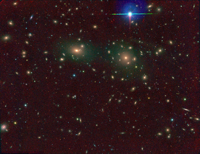
Figure 1: A $UVK$ color image of the Coma field used in the present study: here $U$ is ‘blue’, $V$ is ‘green’ and $K$ is ‘red’. The image is centered on approximately 12:59:52.8 +27:55:00 (J2000) and subtends $29.2^{\prime}$ (RA) $\times 22.5^{\prime}$ (dec). North is up, and east is to the left. The calibrated fits image mosaics are available at NOAO archives.

The exposure time per frame was 15 seconds for $J$ and $K_{s}$ and 10 seconds for $H$. The mosaic corners were only sampled once, other positions along the edge were sampled twice, and positions more than $133^{\prime\prime}$ from the edge of the mosaic were sampled four times, resulting in a nominal total exposure time over most of the field of 60 s, 40 s and 60 s in $J$, $H$ and $K_{s}$ respectively. Figure 1 shows a $UVK$ mosaic of the entire survey region produced from our data.

The images, which were taken using double correlated sampling, were linearized using an empirical correction developed for each pixel, and then flat fielded. A $7\times 7$ grid of observations of M67 was used to determine the type of flat field exposure which minimized the photometric dispersion in measurements of the same stars at many locations across the array. For $J$ and $H$ median sky flats worked best, while for $K_{s}$ an average of dome flats with ambient illumination (i.e. lights off) minimized the dispersion, which was $\approx 2\%$ for all three bands. Next the DIMSUM package within IRAF was used to carry out sky subtraction and masking of bad pixels and cosmic ray hits. For each frame, DIMSUM calculates a median sky frame from preceding and following frames, masking pixels associated with detectable objects. In the $J$ band a median of 10 surrounding frames while rejecting the 2 highest and 2 lowest values at each pixel was found to produce the most uniform appearance across the final mosaicked image. For $H$ a median of 14 frames with rejection of the 3 highest and 3 lowest pixels worked best. For $K_{s}$ an 8 frame median and rejecting 2 high and 2 low pixels was used for the top and bottom third of the mosaic. Because of the large extent of the two dominant central galaxies (NGC 4874 and 4889), in the center three rows of the mosaic DIMSUM tended to oversubtract the sky, and using a median which rejected a larger number of frames substantially alleviated this problem. Nevertheless the extended emission near these two galaxies has probably been suppressed to some extent.

Registration of each sky-subtracted frame to the nearest half pixel was accomplished using offsets measured from objects which overlapped with those in frames to the south or east. The resulting three IR mosaics were registered to one another and rebinned to a common pixel size of $0.6845^{\prime\prime}$ using astrometry for 78 HST Guide Star Catalog objects within the field. In the process the pixel scale for IRIM on the KPNO 2.1 m was determined to be 1.0996, 1.0964, and 1.0922 $\pm 0.0005$ arcseconds per pixel in $J$, $H$ and $K_{s}$ respectively.

Multiple observations of five UKIRT standards transformed to the CIT system (Elias et al., 1982), established that the IR data were photometric, and that the extinction coefficients were 0.17, 0.07, and 0.09 magnitudes per airmass in $J$, $H$ and $K_{s}$ respectively. The Coma mosaic data were all obtained at airmass $<1.15$. Comparison with the infrared photometry of Persson, Frogel & Aaronson (1979) (see below) showed no convincing evidence for a color term, but did reveal the need for a correction of $2-4\%$ for light lost in the small ($5.5^{\prime\prime}$ diameter) apertures used in measuring the relatively faint UKIRT standard stars. This aperture correction was determined empirically from an average of over 50 brighter stars in the standard star images. The zeropoints are judged to be accurate to $\pm 0.03$ magnitudes.

2.2 Optical Data

Optical data were obtained during service observations by George Jacoby at the KPNO 0.9 m telescope on 15 and 16 March 1994 using a 2048² CCD with $0.680^{\prime\prime}$ pixels. Exposures in $B$, $V$, $R$, $I$ were obtained in two positions to cover the infrared mosaic, whereas three positions were used for $U$ and $z$. The total exposure times were 5400s in $U$, 1200s in $B$, 500s in $V$ and $R$, 300s in $I$ and 1800s in $z$. Reduction was carried out in the standard way for these images. The $I$ and $z$ images were obtained in photometric conditions and calibrated using observations of Landolt (1992) and Thuan & Gunn (1976) standards. The $z$ band transformations are judged to be accurate to only $\pm 0.15$ mag. Non–photometric data in $B$, $V$ and $R$ were recalibrated using observations of a $9.7^{\prime}\times 9.7^{\prime}$ portion of the Coma field and of 25 standards obtained in photometric conditions with the COSMIC instrument (using a 2048² CCD with $0.2846^{\prime\prime}$ pixels) on the Palomar 200 inch telescope on 2 February 1995. The $U$ band images from Kitt Peak were calibrated by matching photometry in large apertures on galaxies whose $U$ photometry was published by Bower et al. (1992). The optical and infrared images were registered to a common coordinate system, degraded to the same resolution ($0.6845^{\prime\prime}$ per pixel) and blurred to the seeing of the worst image ($1.7^{\prime\prime}$ FWHM). The reduced and calibrated FITS files for the optical and infrared mosaics will be made publicly available through the NOAO Data Products Program.

2.3 Photometry

We used FOCAS (Jarvis & Tyson, 1981; Valdes, 1982) on the $J$ and $H$ images to produce two independent catalogs. The detection limit was chosen to be 3.5$\sigma$ above the sky level in an area equal to the PSF disk. The two catalogs were position matched to eliminate false detections. Only objects present in both catalogs were accepted in the final catalog (under the assumption that Coma galaxies have similar infrared colors so that the $J$ and $H$ images reach similar depths).

Astrometry for catalogued objects was determined using bright galaxies to establish an initial solution using the IRAF task ccmap. This solution was then used to identify $\sim 50$ objects in the catalog with $H<15$ which were classified as stars by Lobo et al. (1997). These stars were then used to determine the final astrometric solution, which had residual errors of 0.4 arcsec. Catalogued objects were identified with objects in existing catalogs if their positions agreed to within 3 arcseconds, using NED and Lobo et al. (1997)

The angular size of galaxies in the catalog varies widely, requiring the use of an adaptive aperture size for photometry. Simple single aperture photometry would introduce excessive noise for faint objects if the aperture used is too large, or omit substantial light from larger galaxies in the opposite case. An additional problem is deciding which light should be associated with which galaxy, particularly in the central regions where galaxies are clearly overlapping.

Software designed for analysis of faint galaxies in moderately crowded fields was kindly provided to us by Drs. L. Infante and C. J. Pritchet of the University of Victoria (Infante, 1987), containing provisions for a (simple) excision of contaminating objects. For each object Kron (1980) image moments $r_{1}$ and $r_{-2}$ were computed, where $r_{1}$ is the first moment of the light profile and hence a measure of galaxy size, while $r_{-2}$ measures compactness and is defined by the deviation of the area of the galaxy under the light profile from a point spread function.

Photometry in apertures of radius $2r_{1}$ is found to enclose most ($>96\%$) of the total light (Infante, 1987). These apertures vary from object to object and may change from band to band. From simulations with $r^{1/4}$ profiles, it was found necessary to ensure that the measurement aperture within which $r_{1}$ was determined had a radius at least $5\times$ larger than $r_{1}$ to achieve a convergent value of $r_{1}$. For some of the brightest and largest objects this was impractical. For the brightest 10 galaxies 50 kpc (diameter) apertures were adopted to approximate total magnitudes. Model light profiles were fit to the brightest two galaxies (# 1 and 3) and to the brightest star and the resulting models subtracted before measuring photometry on the remaining objects. For the galaxies with $11\lesssim H\lesssim 13$ fixed 30 kpc (diameter) apertures were used (for consistency with Stanford et al. 1995, 1998). For fainter objects $2r_{1}$ apertures were used. These choices were found to be best in terms of photometric accuracy, stability, and noise.

Star-galaxy separation was determined using the classification by Lobo et al. (1997) which uses optical data taken in good seeing, and reaches $V=22.5$. The only objects identified in the present catalog not found in other catalogs were numbers 66, 225 and 711, all of which were outside the Lobo et al. (1997) area (which does not cover RA $>$ 13:00:30 and Dec $<$ 27:49:13 in the present survey area). Star-galaxy separation in the region not surveyed by Lobo et al. (1997) was determined using the $r_{-2}$ compactness parameter Kron (1980).

3 Photometric catalog

Table 1 presents our catalog of objects. In column 1 we show our ID number, in order of decreasing $H$ luminosity (see discussion for Table 2 below). Equatorial coordinates (J2000) are given in columns 2 and 3. Column 4 shows our $H$ magnitude. Column 5 gives the classification as star or galaxy, or if available its morphological type taken from Dressler (1980); Rood & Baum (1967); Caldwell et al. (1993); Graham & Guzman (2003) or the classification shown in the Nasa Extragalactic Database (NED) in a few cases (mostly for faint galaxies where the source of the NED classification was unclear). The source for the morphological class is in column 6. Redshifts, compiled from the best values (lowest stated error) in NED, are in column 7. The sources for the redshifts are given in column 8. Identification numbers from the Godwin, Metcalfe & Peach (1983) catalog are given in column 9. Cross identifications from the NGC, IC, Rood & Baum (1967) and Dressler (1980) catalogs are shown in column 10. Notes on some objects are in column 11. We present the first lines of this table in the printed version, the remainder being available in electronic format.

Table 2 summarizes our estimates of total magnitude in all the bands. The layout of this table is repeated for all photometry tables to follow: in column order we give our ID, $U$, $B$, $V$, $R$, $I$, $z$, $J$, $H$ and $K$. Again, we show the first few lines of this table and make the rest available electronically.

Tables 3-8 show the same information for apertures of $2.1^{\prime\prime},$4.2”, $6.2^{\prime\prime}$, $8.3^{\prime\prime}$, $10.3^{\prime\prime}$ (radius) and $r_{1}$. The aperture magnitudes (50 kpc and 30 kpc) for the brightest objects are reported in Table 2. Finally, by way of example, we show total $H$ magnitudes and $6.2^{\prime\prime}$ aperture colors for 8 colors of common astrophysical interest in Table 9 (first few lines in the printed version, with the rest of the table being made available electronically).

Magnitude errors were estimated via bootstrap simulations. Representative galaxies over a six magnitude range in each band were replicated twenty times on a grid in the image, and their magnitudes extracted. At a total magnitude of $H\sim 15$ a signal to noise of 5 was achieved, consistent with expectations. Table 10 gives functional forms for the variations of the error with magnitude in the $6\farcs 2$ aperture, of the form $\sigma_{band}=\exp(a*(mag)-b)$, where ’‘mag’ is the magnitude in the filter ‘band’. Simulations in which galaxies with known magnitudes and $r_{1}$ were replicated and added to the data show that the catalog is at least 90% complete to H=16.5 for $r_{1}\leq 2.05^{\prime\prime}$, and at least 80% complete to H=16 for $r_{1}\leq 4.1^{\prime\prime}$.

3.1 Comparison with previous photometry

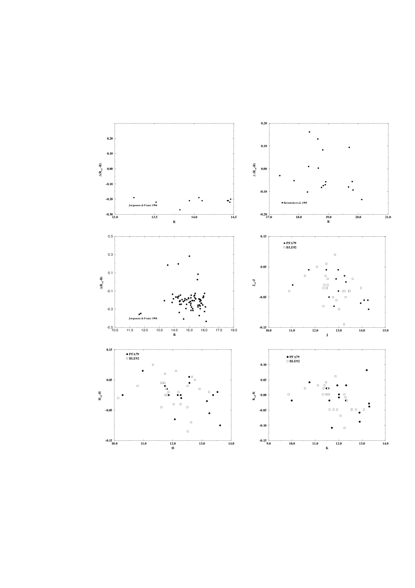
Figure 2: Continued

Table 11 compares our photometry to previous work. Where possible, we derived magnitudes in exactly the same apertures as the comparison measurements. The only exceptions are for Doi et al. (1995) and Lobo et al. (1997), who quote isophotal magnitudes. For these we computed magnitudes in a circular aperture having radius equivalent to the semi-major axis of the limiting isophote. Figure 2 shows the comparisons between the reference photometry and our data.

Our photometry is generally within 2–3% of the reference magnitudes. Small differences in the central filter bandpass and calibration errors can easily account for discrepancies at a few percent level. However, we find a difference of 0.16 mags between our $U$ band data (and those of Bower et al. 1992) and the photographic photometry of Strom & Strom (1978)). We also find a difference of 0.26 mags between our work and Strom & Strom (1978) in $R$, and of 0.21 magnitudes between this work and the Cousins $R$ data of Secker et al. (1997) and Jørgensen & Franx (1994). Our photometry agrees with the Harris $R$ magnitudes of Bernstein et al. (1995), taken with the same filter/detector combination, within 2%.

We convolve the spectral energy distribution of a typical early-type galaxy, with the sensitivity function for the detector used and the filter bandpass, to derive predicted offsets in magnitude between our data and the comparison work used. In the $R$ band, we find that the predicted difference between our photometry and the work of Jørgensen & Franx (1994) and Secker et al. (1997) is $-0.172$ magnitudes, in good agreement with the $-0.210$ we measure. For the 127-04 emulsion and RG610 filter used by Strom & Strom (1978), we find a discrepancy of $-$0.26, identical to the observed value. Similarly, for the IIIa-J emulsion and UG-2 filter used by Strom & Strom (1978) in the $U$, we predict a difference of 0.188 magnitudes, which compares well with the 0.156 magnitudes found. Applying these corrections, our data lie within a few percent of all previous photometry. When we compare with Lobo et al. (1997) we also find a difference of 0.08 magnitudes in the $V$ band: however, the different photometric methods employed (isophotal apertures vs. circular ones) are at least as important as differences in filter bandpasses and detectors.

To facilitate comparisons to our photometry, we provide the response functions for our bands in tables 13 through 21, including the effects of filter and atmospheric transmission, and quantum efficiency.

4 The color-magnitude relation of early-type galaxies in Coma

As an example application of this dataset we study the color-magnitude relation of early-type (E or S0) galaxies and its intrinsic scatter, for the 8 colors shown in Table 9, using the 111 galaxies brighter than $H=14.5$ where we have a complete sample of cluster members. Morphologies for these galaxies are taken from the compilation of Dressler (1980) or Rood & Baum (1967) in order of preference. Only 7 of these 111 galaxies do not have a morphological classification from these sources and we accordingly do not use them for computation of color-magnitude relations and scatter.

Scodeggio (2001) has suggested that the actual slope of the color magnitude relation is much flatter than measured here (and elsewhere) and that this is due to the use of a fixed aperture for all galaxies rather than an adaptive aperture based on the structural parameters of each galaxy (e.g., using the half-light radius). Because galaxies have internal color gradients, a fixed aperture samples more metal poor populations for the fainter galaxies, thus steepening the color-magnitude trend (which is largely a mass-metallicity trend – Trager et al. 2000; Terlevich et al. 2001).

To examine the effect of color gradients within galaxies on the derived CMR’s, we measured and fit the $U-V$ vs. $V$ CMR using a series of fixed circular apertures with radii ranging from $2\farcs 1$ to $10\farcs 3$. We also used apertures with radii $r_{1}$ and $2\times r_{1}$ where $r_{1}$ is the first moment of the light profile (Kron, 1980) and is calculated for each galaxy. The $r_{1}$ and $2\times r_{1}$ apertures should not be affected by the $1.7^{\prime\prime}$ FWHM seeing, as they are generally considerably larger. The intercept of the CMR is redder for smaller apertures, as expected given the general sense of color gradients that are observed within elliptical galaxies. The slope, however, changes only slightly with aperture size, from $-$0.128 for the smallest aperture to $-$0.085 for $r=2\times r_{1}$. By contrast Scodeggio (2001) finds an essentially flat relation when measured within $r_{e}$ in $U-V$ vs $V$. However, our findings are consistent with the mild color gradients observed for E/S0 galaxies in nearby clusters by Tamura & Ohta (2003).

Although it is important to remember that any derived CMR does depend on the apertures used for the photometry, particularly in its intercept, our basic results concerning the slope and scatter of the CMR are insensitive to the aperture size used, and we therefore restrict our attention to the fixed $6\farcs 2$ radius apertures for the remainder of this paper.

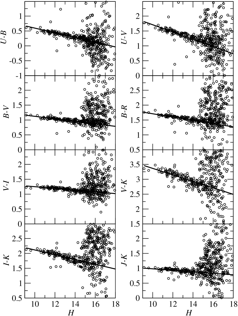
Figure 4: Color-magnitude relations for the eight representative colors tabulated in Table 9. The straight lines show the best fits, whose slopes, intercepts and scatter are tabulated in Table 12.

Figure 3 shows the color-magnitude relations and best linear regression fits for the colors listed in Table 9, vs total $H$ band magnitude. (For reference, $L^{*}$ in the $H$ band is 11.13 (De Propris et al., 1998)). In Figure 4 we show one of these color-magnitude relations using different symbols for members and non-members (the plots in Figure 3 are too compressed to show these clearly).

The slope and intercepts of these fits are shown in Table 12. The intrinsic scatter, also tabulated in Table 12, is calculated using the bootstrap method of Stanford et al. (1995, 1998). One can see that the slope flattens for colors redder than $V$ and that the intrinsic scatter is approximately constant for colors which are equally spaced in (logarithmic) wavelength, suggesting that the relation is indeed driven primarily by metal abundance and that the majority of the stellar populations were formed at early epochs (this is due to the fact that for old stellar populations the only age and metallicity sensitive index lies in the region of the 4000 Å break and the Magnesium complex – see Kodama & Arimoto 1997; Vazdekis et al. 2001).

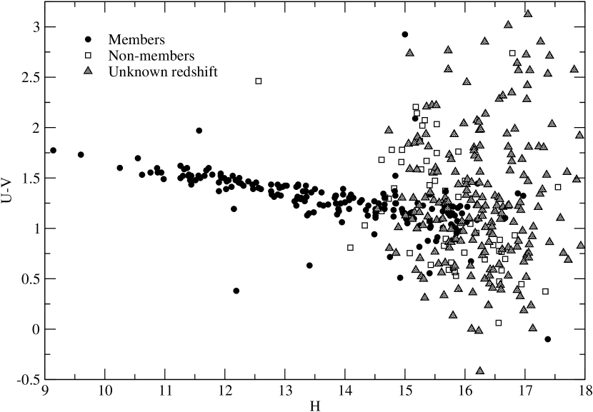
Figure 5: Expanded plot for $U-V$ vs. $H$, showing spectroscopic members, non members and objects with unknown redshifts.

It is also interesting to calculate how the intrinsic scatter varies with galaxy $H$ band luminosity (i.e., stellar mass): Figure 5 shows the variation of the intrinsic scatter in 0.5 mag. bins for four colors. We see no evidence that the intrinsic scatter varies with galaxy luminosity (this may also be appreciated from Figure 3, where the CMR does not appear to spread at faint luminosities).

The existence of a color-magnitude relation is ascribed to a relation between galaxy mass and metallicity, which is suitably explained by models of monolithic collapse followed by fast winds. The small scatter about the relation implies that most of the stellar populations must be quite old and that the timescale for galaxy formation is relatively short, while few mergers may have occurred since early epochs (Bower et al., 1992, 1999). Our observations confirm the small scatter seen by Bower, but also show that the small scatter extends to fainter ellipticals ($\sim L^{*}+3$). This suggests that the stellar populations of all cluster early-type galaxies, irrespective of mass, may have formed rapidly and at high redshift, and that the color-magnitude relation was formed at an early epoch. Indeed, a mature relation is already observed in the $z=0.83$ cluster MS1054-0321 (Andreon, 2006). A similar conclusion was also reached by Andreon et al. (2006) on the basis of their thin color-magnitude relation in Abell 1185. The fact that the intrinsic scatter of the CMR is small for both bright and faint galaxies implies that all red sequence galaxies, irrespective of mass, have undergone a rapid star formation history, in contrast with evidence for ‘downsizing’ among the faint field (and high redshift) galaxy population (Heavens et al., 2004) or for a truncated sequence at higher redshifts (De Lucia et al., 2004).

Table 1: Main catalog of Coma objects

ID	RA (2000)	Dec (2000)	$H$	Type	Ref.	$cz$ (km/s)	Ref.	GMP83	NGC/IC/RB/D	Notes
1	13:00:08.06	27:58:37.4	9.14	Db	D80	6495.	M02	2921.	NGC4889,D148
2	13:00:48.41	27:48:03.6	9.51	star		0.		0.
3	12:59:35.62	27:57:34.1	9.60	cD	D80	7224.	S00	3329.	NGC4874,D129
4	12:58:56.78	27:51:31.4	10.23	star		0.		0.
5	12:59:28.85	27:56:14.4	10.23	star		0.		0.
6	13:00:55.99	27:47:26.6	10.25	Sb	D80	7985.	H97	2374.	NGC4911,D82
7	12:59:20.52	27:51:42.1	10.54	star		0.		0.
8	13:00:54.33	28:00:28.1	10.55	E	D80	8793.	S00	2417.	IC4051,D143
9	13:00:41.60	27:50:39.6	10.62	star		0.		0.
10	12:59:19.80	28:05:03.9	10.62	E	D80	4700.	S04	3561.	NGC4865,D179

Table 2: Total magnitudes for Coma objects

ID (Table 1)	$U$	$B$	$V$	$R$	$I$	$z$	$J$	$H$	$K$
1	13.83	13.27	12.24	11.65	10.91	10.59	9.86	9.14	8.88
2	13.88	13.64	12.79	12.65	11.56	11.54	10.12	9.51	9.76
3	14.24	13.74	12.71	12.12	11.39	11.03	10.37	9.60	9.41
4	13.51	13.47	12.88	12.75	11.78	11.70	10.65	10.23	10.24
5	14.68	14.09	13.20	12.91	11.87	11.82	10.61	10.23	10.20
6	14.12	13.94	13.17	12.60	12.07	11.70	10.94	10.25	9.98
7	16.23	14.97	13.91	13.42	12.34	12.19	11.14	10.54	10.45
8	15.01	14.53	13.62	13.00	12.30	11.98	11.25	10.55	10.41
9	13.20	13.57	12.93	12.87	11.97	11.96	10.91	10.62	10.63
10	15.06	14.68	13.69	13.13	12.44	12.06	11.44	10.62	10.38

Table 3: $2\farcs 1$ Aperture magnitudes for Coma objects

ID (Table 1)	$U$	$B$	$V$	$R$	$I$	$z$	$J$	$H$	$K$
1a	15.94	15.33	13.69	13.10	12.87	12.12	11.79	11.03	10.77
2	13.90	13.69	12.78	12.65	11.62	11.54	10.15	9.58	9.81
3a	16.66	16.09	14.38	13.80	13.67	12.78	12.58	11.81	11.57
4	13.53	13.52	12.88	12.75	11.83	11.70	10.67	10.25	10.27
5	14.70	14.10	13.20	12.91	11.91	11.82	10.63	10.26	10.23
6	17.06	16.59	15.09	14.43	14.11	13.45	13.00	12.27	11.97
7	16.24	15.02	13.91	13.41	12.38	12.19	11.16	10.57	10.48
8	16.95	16.30	14.80	14.20	13.96	13.25	12.80	12.05	11.82
9	13.22	13.62	12.93	12.87	12.02	11.96	10.93	10.65	10.67
10	16.15	15.66	14.31	13.73	13.35	12.72	12.22	11.50	11.29

Table 4: $4\farcs 2$ Aperture magnitudes for Coma objects

ID (Table 1)	$U$	$B$	$V$	$R$	$I$	$z$	$J$	$H$	$K$
1a	15.94	15.33	13.69	13.10	12.87	12.12	11.79	11.03	10.77
2	13.90	13.69	12.78	12.65	11.62	11.54	10.15	9.55	9.81
3a	16.66	16.09	14.38	13.80	13.67	12.78	12.58	11.81	11.57
4	13.53	13.52	12.88	12.75	11.83	11.70	10.67	10.25	10.27
5	14.70	14.12	13.20	12.91	11.91	11.82	10.63	10.26	10.23
6	17.06	16.59	15.09	14.43	14.11	13.45	13.00	12.27	11.97
7	16.24	15.02	13.91	13.41	12.38	12.19	11.16	10.57	10.48
8	16.95	16.30	14.80	14.20	13.96	13.25	12.80	12.05	11.82
9	13.22	13.62	12.93	12.87	12.02	11.96	10.93	10.65	10.67
10	16.15	15.66	14.31	13.73	13.35	12.72	12.22	11.50	11.29

Table 5: $6\farcs 2$ Aperture magnitudes for Coma objects

ID (Table 1)	$U$	$B$	$V$	$R$	$I$	$z$	$J$	$H$	$K$
1a	15.47	14.86	13.70	13.10	12.47	12.12	11.37	10.61	10.34
2	13.88	13.65	12.79	12.65	11.57	11.54	10.12	9.52	9.76
3a	16.12	15.55	14.39	13.80	13.19	12.78	12.10	11.33	11.09
4	13.52	13.48	12.88	12.75	11.79	11.70	10.65	10.23	10.25
5	14.69	14.09	13.20	12.91	11.87	11.82	10.61	10.24	10.21
6	16.70	16.25	15.10	14.43	13.78	13.45	12.65	11.94	11.62
7	16.23	15.00	13.91	13.41	12.35	12.19	11.14	10.55	10.45
8	16.51	15.89	14.81	14.20	13.58	13.25	12.45	11.70	11.46
9	13.20	13.58	12.93	12.87	11.98	11.96	10.91	10.63	10.64
10	15.84	15.34	14.31	13.73	13.09	12.72	11.97	11.26	11.06

Table 6: $8\farcs 3$ Aperture magnitudes for Coma objects

ID (Table 1)	$U$	$B$	$V$	$R$	$I$	$z$	$J$	$H$	$K$
1a	15.24	14.61	13.56	12.96	12.25	11.97	11.14	10.39	10.12
2	13.87	13.64	12.78	12.63	11.55	11.52	10.11	9.51	9.75
3a	15.85	15.28	14.23	13.64	12.94	12.62	11.84	11.08	10.83
4	13.51	13.46	12.87	12.74	11.77	11.69	10.65	10.22	10.24
5	14.68	14.08	13.19	12.90	11.86	11.80	10.61	10.22	10.20
6	16.39	15.97	14.94	14.27	13.55	13.30	12.41	11.70	11.37
7	16.22	15.00	13.90	13.40	12.33	12.18	11.13	10.54	10.44
8	16.26	15.66	14.68	14.07	13.37	13.12	12.24	11.50	11.26
9	13.19	13.56	12.92	12.85	11.96	11.95	10.91	10.62	10.63
10	15.68	15.20	14.22	13.64	12.95	12.63	11.85	11.15	10.95

Table 7: $10\farcs 3$ Aperture magnitudes for Coma objects

ID (Table 1)	$U$	$B$	$V$	$R$	$I$	$z$	$J$	$H$	$K$
1a	15.09	14.48	13.43	12.83	12.12	11.85	11.01	10.25	9.99
2	13.87	13.63	12.77	12.61	11.54	11.50	10.11	9.53	9.74
3a	15.70	15.13	14.08	13.50	12.79	12.46	11.70	10.93	10.69
4	13.51	13.46	12.86	12.73	11.76	11.67	10.64	10.22	10.23
5	14.68	14.08	13.19	12.89	11.85	11.79	10.60	10.22	10.19
6	16.10	15.76	14.78	14.10	13.36	13.12	12.42	11.51	11.18
7	16.22	14.99	13.90	13.39	12.33	12.17	11.13	10.53	10.44
8	16.12	15.53	14.55	13.94	13.24	12.99	12.12	11.37	11.15
9	13.19	13.55	12.91	12.84	11.96	11.93	10.90	10.61	10.62
10	15.61	15.13	14.14	13.56	12.87	12.56	11.78	11.09	10.88

Table 8: $r_{1}$ Aperture magnitudes for Coma objects

ID (Table 1)	$U$	$B$	$V$	$R$	$I$	$z$	$J$	$H$	$K$
1a	15.09	14.48	13.43	12.83	12.12	11.85	11.01	10.25	9.99
2	13.87	13.63	12.77	12.61	11.54	11.50	10.11	9.53	9.74
3a	15.70	15.13	14.08	13.50	12.79	12.46	11.70	10.93	10.69
4	13.51	13.46	12.86	12.73	11.76	11.67	10.64	10.22	10.23
5	14.68	14.08	13.19	12.89	11.85	11.79	10.60	10.22	10.19
6	16.10	15.76	14.78	14.10	13.36	13.12	12.24	11.51	11.18
7	16.22	14.99	13.90	13.39	12.33	12.17	11.13	10.53	10.44
8	16.12	15.53	14.55	13.94	13.24	12.99	12.12	11.37	11.15
9	13.19	13.55	12.91	12.84	11.96	11.93	10.90	10.61	10.62
10	15.61	15.13	14.14	13.56	12.87	12.56	11.78	11.09	10.88

Table 9: Selected colors of Coma galaxies

ID (Table 1)	$H$	$U-B$	$U-V$	$B-V$	$B-R$	$V-I$	$V-K$	$I-K$	$J-K$
1	9.14	0.66	1.83	1.17	1.76	1.28	3.41	2.13	1.03
3	9.60	0.62	1.78	1.17	1.75	1.25	3.35	2.10	1.01
6	10.25	0.50	1.66	1.16	1.83	1.36	3.53	2.16	1.03
8	10.55	0.67	1.75	1.08	1.68	1.28	3.40	2.12	0.99
10	10.62	0.55	1.59	1.03	1.61	1.27	3.30	2.03	0.91
12	10.76	0.55	1.61	1.06	1.66	1.30	3.37	2.07	0.96
14	10.87	0.56	1.65	1.09	1.68	1.28	3.28	2.00	0.89
15	10.88	0.51	1.61	1.10	1.67	1.23	3.28	2.05	0.97
16	10.94	0.57	1.61	1.04	1.65	1.30	3.43	2.13	0.94
17	10.98	0.48	1.55	1.07	1.64	1.25	3.28	2.03	0.99
20	11.26	0.53	1.56	1.02	1.63	1.32	3.40	2.08	1.01
21	11.26	0.56	1.68	1.11	1.67	1.26	3.33	2.07	0.99
23	11.30	0.54	1.57	1.03	1.60	1.29	3.33	2.04	0.99
24	11.32	0.55	1.64	1.09	1.67	1.27	3.32	2.05	1.00
25	11.37	0.54	1.65	1.11	1.69	1.27	3.34	2.07	1.00
26	11.39	0.52	1.58	1.06	1.60	1.24	3.22	1.98	0.98
27	11.40	0.54	1.59	1.05	1.63	1.27	3.28	2.01	0.96
28	11.42	0.47	1.53	1.07	1.63	1.24	3.18	1.94	0.95
29	11.44	0.51	1.58	1.07	1.64	1.24	3.25	2.01	0.94
30	11.44	0.45	1.49	1.05	1.61	1.21	3.14	1.93	0.96

Table 10: Parameters for errors in $6.2^{\prime\prime}$ aperture

Band	$a$	$b$
U	0.582	13.94
B	0.620	15.02
V	0.715	16.25
R	0.647	14.42
I	0.781	15.73
z	0.715	14.61
J	0.909	16.40
H	0.776	13.65
K	0.805	13.81

Table 11: Comparison with previous work

Band	$\Delta$mag (reference $-$ this work)	$\sigma$	Reference
U	0.028	0.037	Bower et al. (1992) – BLE92
	0.156	0.059	Strom & Strom (1978)
B	0.028	0.047	Strom & Strom (1978)
	0.016	0.107	Doi et al. (1995)
V	0.024	0.020	Bower et al. (1992)
	0.019	0.042	Strom & Strom (1978)
	0.078	0.104	Lobo et al. (1997)
R	–0.261	0.108	Strom & Strom (1978)
	–0.020	0.088	Bernstein et al. (1995)
	–0.210	0.134	Jørgensen & Franx (1994)
	–0.213	0.023	Secker et al. (1997)
J	–0.019	0.049	Bower et al. (1992)
	–0.021	0.046	Persson et al. (1979) – PFA79
H	0.010	0.051	Bower et al. (1992)
	–0.002	0.047	Persson et al. (1979)
K	–0.012	0.041	Bower et al. (1992)
	–0.009	0.049	Persson et al. (1979)

Table 12: Color-magnitude relations and scatter

Color	Slope	Intercept	Scatter (measured)	Photometric error	Intrinsic scatter
$U-B$	$-0.079\pm 0.007$	$1.386\pm 0.089$	$0.041\pm 0.005$	$0.016\pm 0.002$	$0.038\pm 0.006$
$U-V$	$-0.122\pm 0.010$	$2.929\pm 0.123$	$0.050\pm 0.004$	$0.016\pm 0.002$	$0.047\pm 0.004$
$B-V$	$-0.042\pm 0.004$	$1.543\pm 0.049$	$0.028\pm 0.004$	$0.008\pm 0.001$	$0.027\pm 0.004$
$B-R$	$-0.055\pm 0.006$	$2.259\pm 0.074$	$0.030\pm 0.004$	$0.008\pm 0.001$	$0.029\pm 0.004$
$V-I$	$-0.029\pm 0.005$	$1.540\pm 0.066$	$0.033\pm 0.003$	$0.010\pm 0.001$	$0.031\pm 0.003$
$V-K$	$-0.109\pm 0.017$	$4.455\pm 0.209$	$0.074\pm 0.010$	$0.015\pm 0.002$	$0.072\pm 0.010$
$I-K$	$-0.080\pm 0.013$	$2.915\pm 0.164$	$0.066\pm 0.009$	$0.012\pm 0.002$	$0.065\pm 0.009$
$J-K$	$-0.025\pm 0.009$	$1.232\pm 0.111$	$0.036\pm 0.006$	$0.016\pm 0.002$	$0.025\pm 0.007$

Table 13: $U$ band response function

Wavelength Å	Throughput %
3050.	0
3100.	0.000117987
3150.	0.0010573
3200.	0.00422111
3250.	0.0142508
3350.	0.0773872
3400.	0.137695
3450.	0.223221
3500.	0.334892
3550.	0.475813

Table 14: $B$ band response function

Wavelength Å	Throughput %
3600.	0
3610.	0
3620.	0.00419808
3630.	0.0147285
3640.	0.021926
3650.	0.0302643
3660.	0.0444033
3670.	0.0587523
3680.	0.0736034
3690.	0.0889334

Table 15: $V$ band response function

Wavelength Å	Throughput
4770.	0
4780.	0.000172793
4790.	0.000690248
4800.	0.0117209
4810.	0.0175596
4820.	0.0259633
4830.	0.0372646
4840.	0.0521359
4850.	0.0710756
4860.	0.0944066

Table 16: $R$ band response function

Wavelength Å	Throughput
5400.	0.00703248
5410.	0.0112412
5420.	0.014039
5430.	0.0281244
5440.	0.0421876
5450.	0.0564394
5460.	0.0707405
5470.	0.0994942
5480.	0.128835
5490.	0.159178

Table 17: $I$ band response function

Wavelength Å	Throughput
6800.	0
6810.	0
6820.	0.000612067
6830.	0.00220244
6840.	0.00476994
6850.	0.00574608
6860.	0.00672227
6870.	0.00782015
6880.	0.0091616
6890.	0.0107461

Table 18: $z$ band response function

Wavelength Å	Throughput %
8000.	0.001212111
8010.	0.001578279
8020.	0.001756357
8030.	0.002116894
8040.	0.002382566
8050.	0.002828275
8060.	0.003360764
8070.	0.003797955
8080.	0.004501144
8090.	0.005287436

Table 19: $J$ band response function

Wavelength Å	Throughput %
10600.00	0
10700.00	0.0121698
10800.00	0.0854674
10900.00	0.478719
11000.00	0.531001
11100.00	0.54874
11200.00	0.00185213
11300.00	0.594653
11400.00	0.452141
11500.00	0.600477

Table 20: $H$ band response function

Wavelength Å	Throughput %
13800.00	0.000337764
14400.00	0.00171936
14500.00	0.00537368
14600.00	0.00819975
14700.00	0.0136237
14800.00	0.0368037
14900.00	0.0946224
15000.00	0.243382
15100.00	0.554612
15200.00	0.756559

Table 21: $K_{s}$ band response function

Wavelength Å	Throughput %
18500.00	0
18600.00	0
18700.00	1.66052e-06
18800.00	0.000684133
18900.00	0
19000.00	0
19100.00	0.00201919
19200.00	0
19300.00	0.00571882
19400.00	0.000896679

Figure 2: Comparison of our photometry with reference photometry (see Table 11) The sources for the comparisons are indicated in the Figure legends.

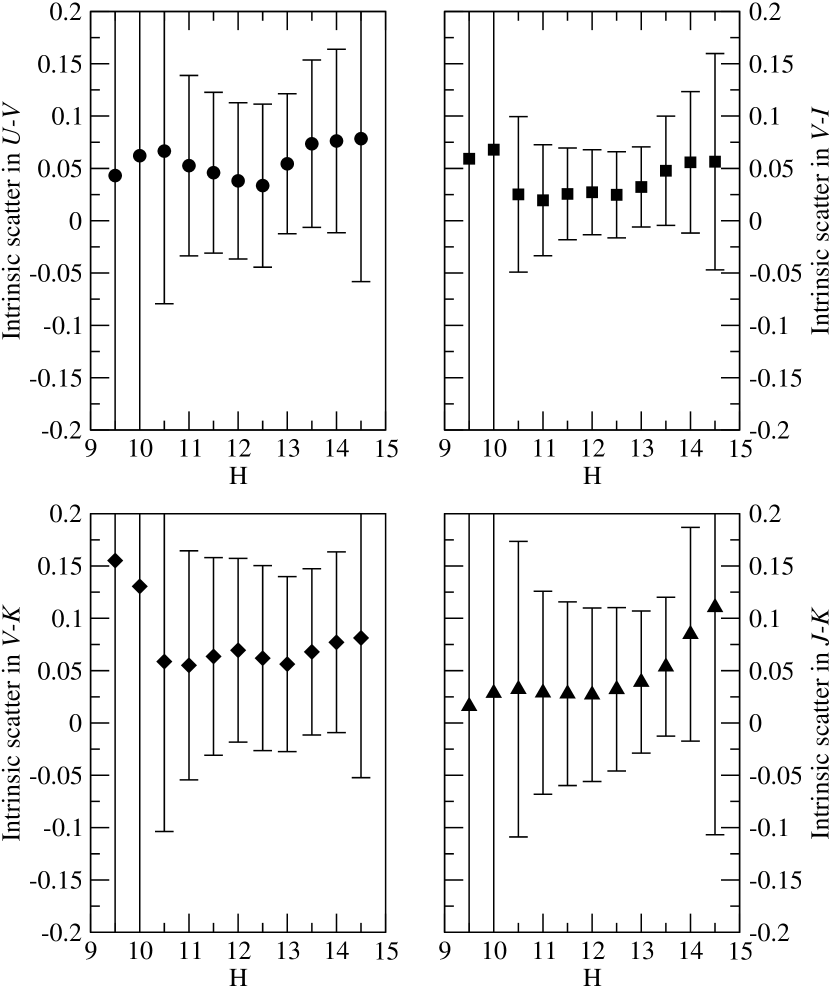
Figure 6: Intrinsic scatter about the color-magnitude relation as a function of $H$-band magnitude, for four colors.

References

- Adami et al. (2000) Adami, C., Ulmer, M. P., Durret, F., Nichol, R. C., Mazure, A., Holden, B. P., Romer, A. K., Savine, C. 2000, A&A, 353, 930
- Andreon (2006) Andreon, S. 2006, MNRAS, 369, 969
- Andreon et al. (2006) Andreon, S., Cuillandre, J.-C., Puddu, E., Mellier, Y. 2006, MNRAS, 372, 60
- Balogh et al. (2004) Balogh, M. et al. 2004, MNRAS, 348, 1355
- Bell & deJong (2001) Bell, E. F., de Jong, R. S. 2001, ApJ, 550, 212
- Bernstein et al. (1995) Bernstein, G. M., Nichol, R. C., Tyson, J. A., Ulmer, M. P., Wittman, D. 1995, AJ, 110, 1507
- Biviano et al. (1995) Biviano, A., Durret, F., Gerbal, D., Le Fevre, O., Lobo, C., Mazure, A., Slezak, C. 1995, A&AS, 111, 265
- Bower et al. (1992) Bower, R. G., Lucey, J. R., Ellis, R. S. 1992, MNRAS, 254, 601 (BLE92)
- Bower et al. (1999) Bower, R. G., Kodama, T., Terlevich, A. 1999, MNRAS, 299, 1193
- Blakeslee et al. (2003) Blakeslee, J. P. et al. 2003, ApJ, 596, L143
- Caldwell et al. (1993) Caldwell, N., Rose, J. A., Sharples, R. M., Ellis, R. S., Bower, R. G, 1993, AJ, 106, 473
- Casoli et al. (1996) Casoli, F., Dickey, J., Kazes, I., Boselli, A., Gavazzi, G., Jore, K. 1996, A&AS, 116, 193
- Castander et al. (2001) Castander, F. et al. 2001, AJ, 121, 2331
- Colless & Dunn (1996) Colless, M. M. & Dunn, A. M. 1996, ApJ, 458, 435
- De Lucia et al. (2004) De Lucia, G. et al. 2004, ApJ, 610, L77
- De Propris et al. (1998) De Propris, R., Eisenhardt, P. R., Stanford, S. A., Dickinson, M. 1998, ApJ, 503, L45
- De Propris et al. (1999) De Propris, R., Stanford, S. A., Eisenhardt, P. R., Dickinson, M., Elston, R. 1999, AJ, 118, 719
- Doi et al. (1995) Doi, M., Fukugita, M., Okamura, S., Turner, E. L. 1995, AJ, 109, 1490
- Dressler (1980) Dressler, A. 1980, ApJS, 42, 565 (D)
- Dressler & Shectman (1988) Dressler, A. & Shectman, S. A. 1988, AJ, 95, 284
- Edwards et al. (2002) Edwards, S. A., Colless, M., Bridges, T. J., Carter, D., Mobasher, B., Poggianti, B. M. 2002, ApJ, 567, 178
- Elias et al. (1982) Elias, J. H., Frogel, J. A., Matthews, K., Neugebauer, G. 1982, AJ, 87, 1029
- Eggen et al. (1962) Eggen, O. J., Lynden-Bell, D., Sandage, A. 1962, ApJ, 136, 748
- Ellis et al. (2006) Ellis, S. C., Jones, L. R., Dononvan, D., Ebeling, H., Khosroshahi, H. G. 2006, MNRAS, 368, 769
- Gavazzi et al. (1996) Gavazzi, G., Pierini, D., Boselli, A. 1996, A&A, 312, 397
- Godwin et al. (1983) Godwin, J. G., Metcalfe, N., Peach, J. V. 1983, MNRAS, 202, 113 (GMP83)
- Graham & Guzman (2003) Graham, A. W. & Guzman, R. 2003, AJ, 125, 2936
- Haynes et al. (1997) Haynes, M. P., Giovanelli, R., Herter, T., Vogt, N. P., Freudling, W., Maia, M. A. G., Salzer, J. J., Wegner, G. 1997, AJ, 113, 1197
- Heavens et al. (2004) Heavens, A., Panter, B., Jimenez, R., Dunlop, J. 2004, Nature, 428, 625
- Holden et al. (2004) Holden, B. P., Stanford, S. A., Eisenhardt, P. R., Dickinson, M. 2004, AJ, 127, 2484
- Holden et al. (2006) Holden, B. P. et al. 2006, ApJ, 642, L123
- Infante (1987) Infante, L. 1987, A&A, 183, 177
- Jarvis & Tyson (1981) Jarvis, J. F. & Tyson, J. A. 1981, AJ, 86, 476
- Jørgensen & Franx (1994) Jørgensen, I. & Franx, M. 1994, ApJ, 433, 553
- Kajisawa et al. (2000) Kajisawa, M. et al. 2000, PASJ, 52, 61
- Kaviraj et al. (2005) Kaviraj, S., Devriendt, J. E. G., Ferreras, I., Yi, S. K. 2005, MNRAS, 360, 60
- Kodama & Arimoto (1997) Kodama, T. & Arimoto, N. 1997, A&A, 320, 41
- Kron (1980) Kron, R. G. 1980, ApJS, 43, 305
- Landolt (1992) Landolt, A. U. 1992, AJ, 104, 340
- Lobo et al. (1997) Lobo, C., Biviano, A., Durret, F., Gerbal, D., Le Fevre, O., Mazure, A., Slezak, E. 1997, A&AS, 122, 409
- Lopez-Cruz et al. (2004) Lopez-Cruz, O., Barkhouse, W., Yee, H. K. C. 2004, ApJ, 614, 679
- Lidman et al. (2004) Lidman, C., Rosati, P. Demarco, R., Nonino, M., Mainieri, V., Stanford, S. A., Toft, S. 2004, A&A, 416, 829
- Matkovic & Guzman (2005) Matkovic, A. & Guzman, R. 2005, MNRAS, 362, 289
- McIntosh et al. (2005) McIntosh, D. H., Zabludoff, A. I., Rix, H.-W., Caldwell, N. 2005, ApJ, 619, 193
- Mei et al. (2006a) Mei, S. et al. 2006a, ApJ, 639, 81
- Mei et al. (2006b) Mei, S. et al. 2006b, ApJ, 644, 759
- Mobasher et al. (2001) Mobasher, B. et al. 2001, ApJS, 137, 279
- Moore et al. (2002) Moore, S. A. W., Lucey, J. R., Kuntschner, H., Colless, M. M. 2002, MNRAS, 336, 382
- Müller et al. (1999) Müller, K. R., Wegner, G., Raychaudhury, S., Freudling, W. 1999, A&AS, 140, 327
- Persson et al. (1979) Persson, S. E., Frogel, J. A., Aaronson, M. 1979, ApJS, 39, 61 (PFA79)
- Renzini (2006) Renzini, A. 2006, ARA&A, 44, 141
- Rood & Baum (1967) Rood, H. J. , Baum, W. A. 1967, AJ, 72, 398
- Sandage & Visvanathan (1978) Sandage, A. & Visvanathan, N. 1978, ApJ, 223, 707
- Scodeggio (2001) Scodeggio, M. 2001, AJ, 121, 2413
- Secker et al. (1997) Secker, J., Harris, W. E., Plummer, J. D. 1997, PASP, 109, 1377
- Shioya et al. (2002) Shioya, Y., Bekki, K., Couch, W., De Propris, R. 2002, ApJ, 565, 223
- Smith et al. (2000) Smith, R. J., Lucey, J. R., Hudson, M. J., Schlegel, D. J., Davies, R. L. 2000, MNRAS, 313, 469
- Smith et al. (2004) Smith, R. J. et al. 2004, AJ, 128, 1558
- Stanford et al. (1995) Stanford, S. A., Eisenhardt, P. R., Dickinson, M. 1995, ApJ, 450, 512
- Stanford et al. (1998) Stanford, S. A., Eisenhardt, P. R,, Dickinson, M. 1998, ApJ, 492, 461
- Strazzullo et al. (2006) Strazzullo, V. et al. 2006, A&A, 450, 909
- Strom & Strom (1978) Strom K. M. & Strom S. E. 1978, AJ, 83, 73
- Tamura & Ohta (2003) Tamura, N. & Ohta, K. 2003, AJ, 126, 596
- Terlevich et al. (2001) Terlevich, A. I., Caldwell, N., Bower, R. G. 2001, MNRAS, 326, 1547
- Thuan & Gunn (1976) Thuan, T. X. & Gunn, J. E. 1976, PASP, 88, 543
- Trager et al. (2000) Trager, S. C., Faber, S. M., Worthey, G., Gonzalez, J. J. 2000, AJ, 120, 165
- Valdes (1982) Valdes, F. 1982, in Instrumentation in Astronomy IV, Proc. SPIE, 331, 465
- van Dokkum et al. (2000) van Dokkum, P. G., Franx, M., Fabricant, D., Illingworth, G. D., Kelson, D. D. 2000, ApJ, 541, 95
- van Dokkum et al. (2001) van Dokkum, P. G., Stanford, S. A., Holden, B. P., Eisenhardt, P. R., Dickinson, M., Elston, R. 2001, ApJ, 552, L101
- Vazdekis et al. (2001) Vazdekis, A., Kuntschner, H., Davies, R. L., Arimoto, N., Nakamura, O., Peletier, R. 2001, ApJ, 551, L127
- Wake et al. (2005) Wake, D. A., Collins, C. A., Nichol, R. C., Jones, L. R., Burke, D. J. 2005, ApJ, 627, 186