The Galactic positron flux and dark matter substructures

Abstract

In this paper we calculate the Galactic positron flux from dark matter annihilation in the frame of supersymmetry, taking the enhancement of the flux by existence of dark matter substructures into account. The propagation of positrons in the Galactic magnetic field is solved in a realistic numerical model GALPROP. The secondary positron flux is recalculated in the GLAPROP model. The total positron flux from secondary products and dark matter annihilation can fit the HEAT data well when taking a cuspy density profile of the substrctures.

Keywords: dark matter, positron, propagation

1 Introduction

The astronomical observations indicate that most of the matter in our universe is dark (see for example [1]). The evidences come mainly from the gravitational effects of the dark matter component, such as the rotation curves of spiral galaxies [2], the gravitational lensing [3] and the dynamics of galaxy clusters [4]. The studies of primordial nucleosynthesis [5], structure formation [6] and cosmic microwave background (CMB) [7] show that this so-called dark matter (DM) is mostly non-baryonic. The nature of the non-baryonic dark matter remains one of the most outstanding puzzles in particle physics and cosmology.

A large amount of theoretical models of DM have been proposed in literatures [8]. All these candidates of non-baryonic DM particles require physics beyond the standard model of particle physics. Among the large amount of candidates, the most attractive scenario involves the weakly interacting massive particles (WIMPs). In particular, the minimal supersymmetric extension of the standard model (MSSM) provides an excellent WIMP candidate as the lightest supersymmetric particle (LSP), usually the neutralino, which are stable due to R-parity conservation [1].

WIMPs are possible to be detected beyond the gravitational effects. One viable way is to detect the elastic scattering signals of DM particles on the detector nuclei (direct searches) [9, 10, 11, 12]. This is the most sensitive method at present for DM detection [13]. Another way is to search the self-annihilation prodcuts of the DM particles (indirect searches), such as neutrinos [14], $\gamma$-rays [15, 16], antiprotons [17] and positrons [18, 19]. Since the positrons, antiprotons and diffuse $\gamma$-rays are secondary particles in the cosmic rays with low fluxes, these kinds of DM annihilation products are easier to be distinguished from the astrophysical background. Direct and indirect detections of DM particles are complementary ways to each other.

The balloon-borne instrument High-Energy Antimatter Telescope (HEAT) was designed to determine the positron fraction over a wide energy range with high statitical and systematic accuracy. Based on the three flights(1994, 1995 and 2000), this collaboration reported an excess of positrons with energies higher than several $GeV$ and peaked in the range $7\sim 10\ GeV$ [20, 21]. It seems that the astrophysical production cannot give enough positrons as observed [22], and there might exist exotic sources of positrons. It has been pointed out that the excess may indicate the signal of DM annihilation [18, 19]. However, Baltz et alshowed that for supersymmetry (SUSY) DM a “boost factor” $\geq 30$ has to be introduced to fit the HEAT data [23]. It was thought that the local clumpiness of DM distribution might account for this “boost factor”. However, Hooper et alargued that it was less possible for a DM clump to be close enough to the Earth to contribute sufficient positron flux [24].

Stimulated by the recent numerical simulation which shows that the lightest subhalos in the Galaxy could be extended to $10^{-6}M_{\odot}$ with a huge amount of about $10^{15}$ [25], we try to calculate the Galactic positron flux again in the frame of supersymmetry taking the enhancement by the large amount of subhalos into account. There was effort try to explain the HEAT data by the nearby mini-clumps [26]. However, the possibility of this scenario is also extremely low [27]. Another difference of this work from the previous studies most of which adopt the Green’s function method to calculate the positron’s propagation is that we calculate its propagation in the Galactic magnetic field using the numerical package GALPROP [28], which adopts realistic distribution of interstellar gas and radiation field. Our result shows that the two methods lead to some difference. To give a consistent result we also calculate the secondary positron flux using GALPROP. The propagation parameters are adjusted to fit observations such as B/C, proton and electron spectra. Our results show that the secondary positron has better agreement with the HEAT data than which adopted in previous studies [18, 19, 23, 26] and decreases the tension between predictions and data.

The paper is orgnized as following: in Sec. 2 we present the SUSY model. In Sec. 3 we give our treatment of subhalos distribution and density profiles. Sec. 4 introduces the positron’s propagation and the GALPROP model. The results are given in Sec. 5.

2 Positron Production from Neutralino Annihilation

The LSP, generally the lightest neutralino, is stable in the R-parity conservative MSSM and provides a natural candidate of dark matter. It is a combination state of the supersymmetric partners of the photon, $Z^{0}$ boson and neutral Higgs bosons.

Positrons can be produced in several neutralino annihilation modes. Most of them come from the decay of gauge bosons produced in chanels $\chi\chi\rightarrow ZZ,\ \chi\chi\rightarrow W^{+}W^{-}$, or from the cascades of final particles, such as fermions and Higgs bosons. The spectrum of positrons depends on the neutralino mass and its annihilation modes. There is also a direct channel $\chi\chi\rightarrow e^{+}e^{-}$ and produces monochrome positrons with energy $E_{e^{+}}=m_{\chi}$. However, the branching ratio of this channel is usually small. In the following discussion we neglect this “line” contribution to the positron spectrum.

The source function of positrons from DM annihilation can be written as

$$Q(E_{e^{+}},{\bf r})=\frac{\langle\sigma v\rangle}{2m_{\chi}^{2}}\frac{{\rm d}n}{{\rm d}E}\rho^{2}({\bf r}),$$ (1)

where $\sigma$ is the positron generating cross-section, ${{\rm d}n}/{{\rm d}E}$ is the positrons spectrum in one annihilation by a pair of neutralinos and $\rho({\bf r})$ is neutralino density distribution in space. The source term $Q(E_{e^{+}},{\bf r})$ is given in unit of $GeV^{-1}m^{-3}s^{-1}$.

The source term is calculated in MSSM by doing a random scan using the software package DarkSUSY [29]. In these SUSY models we choose a few models which satisfy all the experimental bounds and give large fluxes and appropriate spectrum so that we can fit the HEAT data well. However, there are more than one hundred free SUSY breaking parameters even for the R-parity conservative MSSM. A general practice is to assume some relations between the parameters and greatly reduce the number of free parameters. For the processes related with dark matter production and annihilation, only seven parameters are relevant under some simplifying assumptions, i.e., the higgsino mass parameter $\mu$, the wino mass parameter $M_{2}$, the mass of the CP-odd Higgs boson $m_{A}$, the ratio of the Higgs Vacuum expectation values $\tan\beta$, the scalar fermion mass parameter $m_{\tilde{f}}$, the trilinear soft breaking parameter $A_{t}$ and $A_{b}$. To determine the low energy spectrum of the SUSY particles and coupling vertices, the following assumptions have been made: all the sfermions have common soft-breaking mass parameters $m_{\tilde{f}}$; all trilinear parameters are zero except those of the third family; the bino, wino, and gluino have the mass relations, $M_{1}=5/3\tan^{2}\theta_{W}M_{2}$, $M_{3}=\alpha_{3}(M_{Z})/{\alpha_{\mbox{em}}}\sin^{2}\theta_{W}M_{2}$, coming from the unification of the gaugino mass at the grand unification scale.

The parameters are constrained in the following ranges: $50GeV<|\mu|,\ M_{2},\ M_{A},\ m_{\tilde{f}}<10TeV$; $1.1<\tan\beta<55$; $-3m_{\tilde{q}}<A_{t},\ A_{b}<3m_{\tilde{q}}$; $\mbox{sign}(\mu)=\pm 1$. The SUSY models are required to satisfy the theoretical consistency requirement, such as the correct vacuum breaking pattern, the neutralino being the LSP and so on. The accelerator data constrains the models further from the spectrum requirement, the invisible Z-boson width, the branching ratio of $b\to s\gamma$ and the muon magnetic moment.

The constraint from cosmology is also taken into account by requiring the relic abundance of neutralino $0.091<\Omega_{\chi}h^{2}<0.118$, which corresponds to the 3$\sigma$ bound from the cosmological observations [7]. The effect of coannihilation between the fermions is taken into account when calculating the relic density numerically.

3 Dark Matter Distribution

To determine the positron source term from DM annihilation in Eq. (1) we have to specify the DM density profile $\rho({\bf r})$. Based on the N-body simulation results the DM density profile can be written in a general form as [30]

$$\rho=\frac{\rho_{s}}{(r/r_{s})^{\gamma}[1+(r/r_{s})^{\alpha}]^{(\beta-\gamma)/\alpha}},$$ (2)

where $\rho_{s}$ and $r_{s}$ are the scale density and scale radius respectively. These two parameters are determined by the measurement of the virial mass of the halo and the concentration parameter determined by simulation. The NFW profile was first proposed by Navarro, Frenk and White [31] with $(\alpha,\beta,\gamma)=(1,3,1)$. However, Moore et al. gave another form of DM profile with $(\alpha,\beta,\gamma)=(1.5,3,1.5)$ to fit their simulation result [32]. The Moore profile has steeper slope near the Galactic center than the NFW profile. There are also simulations showing that the density profile may not be universial [33, 34]. Reed et al. show that $\gamma=1.4-0.08\log(M/M_{*})$ increases for halos with smaller masses [34]. Therefore we also adopt a $\gamma=1.7$ profile for the whole range of DM halos for simplicity. At present there are controversials on which one represents the actual density profile.

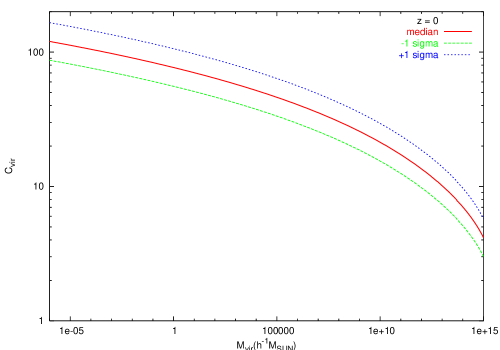
Figure 1: $c_{\mbox{vir}}$ as a function of subhalo mass $m_{\mbox{sub}}$ predicted by the Bullock model [35]. The median and the 1$\sigma$ values are given.

For a DM halo with mass $M_{\mbox{vir}}$, we adopt a semi-analytic model of Bullock et al[35], which describes the concentration parameter $c_{\mbox{vir}}$ as a function of viral mass and redshift, to determine the parameters in the density profile. We plot the $c_{\mbox{vir}}-M_{\mbox{vir}}$ relation in Figure 1, with the $1\sigma$ range. The median $c_{\mbox{vir}}-M_{\mbox{vir}}$ relation at redshift zero is adopted. The scale radius is then determined as $r^{\mbox{nfw}}_{\mbox{s}}=r_{\mbox{vir}}/c_{\mbox{vir}}$, $r^{\mbox{moore}}_{\mbox{s}}=r^{\mbox{nfw}}_{\mbox{s}}/0.63$ and $r^{\gamma}_{\mbox{s}}=r^{\mbox{nfw}}_{\mbox{s}}/(2-\gamma)$. The virial radius $r_{\mbox{vir}}$ in above formula is defined by $M_{\mbox{vir}}=4\pi\Delta\rho_{\mbox{c}}r_{\mbox{vir}}^{3}/3$ with $\Delta=200$ and the critical density of the universe $\rho_{\mbox{c}}=139M_{\odot}/kpc^{3}$. Once $r_{\mbox{s}}$ is fixed, the scale density $\rho_{\mbox{s}}$ can be got by solving the equation $M_{\mbox{vir}}=\int\rho({\bf r}){\rm d}^{3}{\bf r}$. In Figure 2 we show the scale radius $r_{\mbox{s}}$, scale density $\rho_{\mbox{s}}$, virial radius $r_{\mbox{vir}}$, surface mass density $\rho(r_{\mbox{vir}})$, effective volume $\xi=\int(\rho/\rho_{0})^{2}{\rm d}^{3}{\bf r}$, intrinsic boost factor $B_{\mbox{c}}=\frac{\int(\rho/\rho_{0})^{2}{\rm d}^{3}{\bf r}}{\int(\rho/\rho_{0}){\rm d}^{3}{\bf r}}$ as functions of masses $M_{\mbox{vir}}$, for the DM halos with NFW mass distributions. We adopt a reference mass density $\rho_{0}=0.3GeV/cm^{3}$. Each of these charicteristic quantities is scaled by its maximum value in the mass range $2\times 10^{-6}\sim 2\times 10^{10}M_{\odot}$, the minimal and maximal masses of the Milky Way (MW) subhalos we adopt in the following discussion. We list these scale factors as: $r_{\mbox{s}}^{\mbox{max}}=2.72kpc,\ \rho_{\mbox{s}}^{\mbox{max}}=3.52\times 10^{9}M_{\odot}/kpc^{3},\ r_{\mbox{vir}}^{\mbox{max}}=55.62kpc,\ \rho(r_{\mbox{vir}})^{\mbox{max}}=1.52\times 10^{-4}GeV/cm^{3},\ \xi^{\mbox{max}}=1909.11kpc^{3},\ B_{\mbox{c}}^{\mbox{max}}=39.89.$ The behaviors of these quantities can be understood as following. For NFW profile, an analytic calculation shows that $r_{\mbox{vir}}\propto M_{\mbox{vir}}^{1/3}$, and $r_{\mbox{s}}\propto M_{\mbox{vir}}^{1/3}/c_{\mbox{vir}}$. Because the concentration parameter $c_{\mbox{vir}}$ is weakly dependent on the mass according to Figure 1, $r_{\mbox{s}}$ is approximately proportional to $M_{\mbox{vir}}^{1/3}$. The scale density $\rho_{\mbox{s}}$ is nearly $\propto c_{\mbox{vir}}^{3}/\ln(1+c_{\mbox{vir}})$, which shows a slight decrease as the increase of halo mass, while the surface density $\rho(r_{\mbox{vir}})\sim\rho_{\mbox{(}s)}/c_{\mbox{vir}}^{3}\propto 1/\ln(1+c_{\mbox{vir}})$ is almost constant. The effective volume $\xi$ is approximately scaled with $M_{\mbox{vir}}c_{\mbox{vir}}^{3}$, and the intrinsic boost factor $B_{\mbox{c}}\propto c_{\mbox{vir}}^{3}$. $B_{\mbox{c}}$ is a little smaller for higher mass halos, because it is less concentrated for higher mass halo.

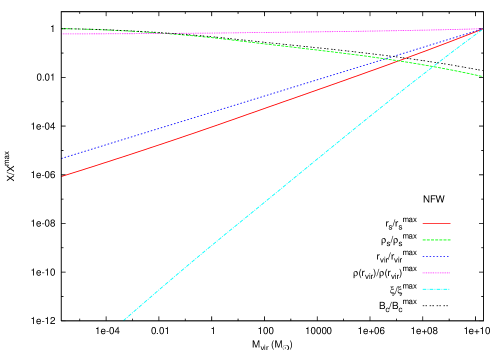
Figure 2: Some characteristic quantities of DM halos with NFW mass distribution as functions of masses.

Having known the general properties of the DM halos given above, we now turn to the discussion of the MW subhalos. High resolution simulations have revealed that a large number of self-bound substructures survived in the galactic halos [36, 37, 38, 39, 40, 41, 42, 43]. Especially a recent simulation conducted by Diemand et al. [25] showed that the first generation objects as light as the Earth mass can survive until today. The number of such minihalos is huge, reaching $10^{15}$. The existence of a wealth of subhalos will greatly enhance the DM annihilation flux, since the annihilation rate is propotional to the density square as shown in Eq. (1).

The simulations show that the number density of subhalos can be approximately given by an isothermal profile with a core [44]

$$n(r)=2n_{H}(1+(r/r_{H})^{2})^{-1}\ ,$$ (3)

where $n_{H}$ is the relative number density at the scale radius $r_{H}$, with $r_{H}$ being about $0.14$ times the halo virial radius $r_{H}=0.14r_{\mbox{vir}}$. The result given above agrees well with that in another recent simulation by Gao et al.[45]. Eq. (3) shows that the radial distribution of substructures is generally shallower than the density profile of the smooth background in Eq. (2). This is due to the tidal disruption of substructures which is most effective near the galactic center.

The mass function is well fitted to the simulation result as ${\rm d}n/{\rm d}m_{\mbox{sub}}\propto m_{\mbox{sub}}^{-1.9}$. We then get the number density of substructures with mass $m_{\mbox{sub}}$ at the position $r$ to the galactic center

$$n(m_{\mbox{sub}},r)=n_{0}\left(\frac{m_{\mbox{sub}}}{M_{\mbox{vir}}}\right)^{-1.9}(1+(r/r_{H})^{2})^{-1}\ ,$$ (4)

where $M_{\mbox{vir}}$ is the virial mass of the MW, $n_{0}$ is the normalization factor determined by requiring the number of subhalos with mass larger than $10^{8}M_{\odot}$ is about 500 in a halo with $M=2\times 10^{12}M_{\odot}$[38].

Taking the subhalos into account the density square in Eq. (1) is given by

$$\rho^{2}({\bf r})\to\langle\rho^{2}({\bf r})\rangle=\rho^{2}_{\mbox{smooth}}({\bf r})+\langle\rho^{2}_{\mbox{sub}}({\bf r})\rangle,$$ (5)

where $\langle\rho^{2}_{\mbox{sub}}({\bf r})\rangle$ means the average density square of subhalos according to the distribution probability. Since there is no correlation between the mass and spatial distribution in Eq. (4) we get $\langle\rho^{2}_{\mbox{sub}}({\bf r})\rangle$ at the position ${\bf r}$ is given by an integral of mass

$$\langle\rho^{2}_{\mbox{sub}}({\bf r})\rangle = \int_{m_{\mbox{min}}}^{m_{\mbox{max}}}n(m_{\mbox{sub}},r)\left(\int\rho_{\mbox{sub}}^{2}{\rm d}V\right)\cdot{\rm d}m_{\mbox{sub}}$$ (6)

$$= \frac{n_{0}}{1+(r/r_{H})^{2}}\int_{m_{\rm min}}^{m_{\rm max}}f(m_{\mbox{sub}})\cdot{\rm d}m_{\mbox{sub}}\ \ ,$$

where $\rho_{\mbox{sub}}$ refers to density of the subhalo at ${\bf r}$ and $V$ is its volume. We defined a function $f(m_{\mbox{sub}})$ in the equation above as

$$f(m_{\mbox{sub}})=\left(\frac{m_{\mbox{sub}}}{M_{vir}}\right)^{-1.9}\int_{0}^{r_{\mbox{\tiny vir}}(m_{\mbox{\tiny sub}})}4\pi{r^{\prime}}^{2}\rho^{2}_{\mbox{sub}}(r^{\prime}){\rm d}r^{\prime},$$ (7)

which depends only on the subhalo mass since the virial radius and the density profile are all determined by the subhalo mass. The minimal subhalos can be as light as $10^{-6}M_{\odot}$ [25] while the maximal mass of substructures is taken to be $0.01M_{\mbox{vir}}$ [46].

We notice that there are unphysical singularities at the center of the subhalo which may lead to $f(m_{\mbox{sub}})$ divergent for the index $\gamma$ equal to or greater than $1.5$. A cutoff $r_{\mbox{cut}}$ is introduced within which the DM density is kept a constant value $\rho_{\mbox{max}}$ due to the balance between the annihilation rate and the rate to fill the region by infalling DM particles [47]. Applying typical setting of parameters, we get $\rho_{\mbox{max}}\sim 10^{18}-10^{19}M_{\odot}/kpc^{3}$. In the following discussion, $\rho_{\mbox{max}}=10^{18}M_{\odot}/kpc^{3}$ is adopted for NFW and Moore profiles while we consider $\rho_{\mbox{max}}=10^{18}-2\times 10^{19}M_{\odot}/kpc^{3}$ for the profile with $\gamma=1.7$.

From Eq. (6) we know that, $\langle\rho^{2}_{\mbox{sub}}\rangle\propto\int f(m_{\mbox{sub}})\,{\rm d}m_{\mbox{sub}}=\int m_{\mbox{sub}}f(m_{\mbox{sub}})\,{\rm d}\ln m_{\mbox{sub}}$. The quantity $m_{\mbox{sub}}\times f(m_{\mbox{sub}})$ is plotted in Figure 3, which shows the relative contribution to the annihilation signals from subhalos at different mass bins at the logarithmic scale. We can see from this figure that subhalos of different mass bins contribute almost the same to the annihilation products. By extending the minimal subhalo mass from the present numerical resolution of about $10^{6}M_{\odot}$ to $10^{-6}M_{\odot}$, the contribution will be $\sim 4$ times larger.

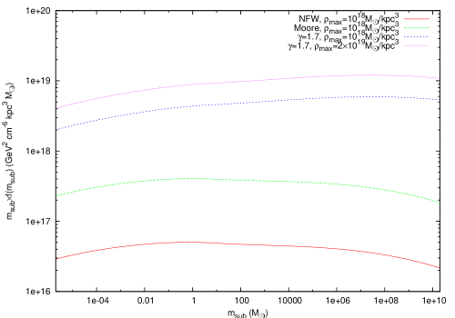
Figure 3: $m_{\mbox{sub}}\times f(m_{\mbox{sub}})$ as a function of subhalo mass $m_{\mbox{sub}}$.

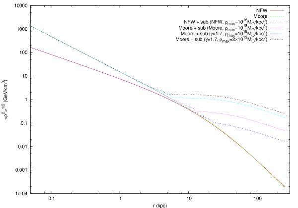
Figure 4: $\langle{\rho^{2}(r)}\rangle^{1/2}$ distribution of Galaxy for various DM profiles.

Figure 4 shows $\langle{\rho^{2}}\rangle^{1/2}$ for different DM profiles. The existence of subhalos will increase $\langle{\rho^{2}}\rangle^{1/2}$ significantly at large radii. Because the annihilation source is density square dependent, the further clumpiness of DM will effectively increase the annihilation signals, and can play the role of a “boost factor”. The more concentrated of the halo profile, the larger of the $\langle{\rho^{2}}\rangle^{1/2}$ value. While at small radii there is no enhancement compared to the smooth component for the tidal disruption makes the subhalos be difficult to survive in inner Galaxy. We can see that the model with the most cuspy subhalos adopted here has $\sim 3$ times larger $\langle{\rho^{2}}\rangle^{1/2}$ than the smooth one at the solar location, which means that the positron flux observed on the Earth will be higher by about an order of magnitude.

4 The Positron Propagation

A complexity in calculating the positron flux is that positrons are scattered by the Galactic magnetic field (GMF) and we have to calculate its propagation in GMF. The propagation of charged particles in the GMF is diffusive. In addition they will also experience energy loss processes due to ionization and Coulomb interaction in the interstellar medium; for electrons and positrons there are additional synchrotron radiation in the GMF, bremsstrahlung radiation in the interstellar medium and inverse Compton scattering in the interstellar radiation field. The interaction between cosmic-ray particles and the interstellar medium (mostly Hydrogen and Helium) will lead to the fragmentation of nuclei. For radioactive nuclei the decay should be also taken into account.

The full propagation equation including the convection of cosmic-ray particles and reacceleration processes is written in the form

$$\frac{\partial\psi}{\partial t} = Q({\bf x},p)+\nabla\cdot(D_{xx}\nabla\psi-{\bf V}\psi)+\frac{\partial}{\partial p}p^{2}D_{pp}\frac{\partial}{\partial p}\frac{1}{p^{2}}\psi$$ (8)

$$- \frac{\partial}{\partial p}\left[\dot{p}\psi-\frac{p}{3}(\nabla\cdot{\rm V}\psi)\right]-\frac{\psi}{\tau_{f}}-\frac{\psi}{\tau_{r}},$$

where $\psi$ is the density of cosmic ray particles per unit momentum interval, $Q({\bf x},p)$ is the source term, $D_{xx}$ is the spatial diffusion coefficient, ${\bf V}$ is the convection velocity. The third term describes the reacceleration using diffusion in momentum space. $\dot{p}$ is the momentum loss rate, $\tau_{f}$ and $\tau_{r}$ are timescales for fragmentation and radioactive decay respectively.

The interaction between cosmic-ray particles and the interstellar medium produces the secondary particles, such as positrons, antiprotons and some other heavy elements. The source term of the secondary cosmic-rays is given by

$$Q({\bf x},p)=\beta c\psi_{p}({\bf x},p)[\sigma_{H}(p)n_{H}({\bf x})+\sigma_{He}(p)n_{He}({\bf x})],$$ (9)

where $\psi_{p}({\bf x},p)$ is the density of primary cosmic-rays, $\beta c$ is the velocity of particles, $\sigma_{H}$ and $\sigma_{He}$ are the production cross sections for the secondary particles from the progenitor on H and He targets, $n_{H}$ and $n_{He}$ are the interstellar Hydrogen and Helium number densities, respectively.

The propagation equation (8) can be solved analytically under some simplification assumptions [18, 48]. A numerical solution to Eq. (8) is given in the GALPROP model developed by Strong and Moskalenko [28], which takes all the relevant processes into account. The realistic distributions for the interstellar gas and radiation fields are adopted in GALPROP. The detail of this model can be found in [28].

The secondary-primary ratio such as B/C depends on the propagation process. Therefore the propagation parameters are adjusted to describe the B/C ratio, the electron and proton spectra et al. We include the nuclei up to $Z=28$ and relevant isotopes. The injection spectra of protons and heavier nuclei are assumed to have the same power-law form in rigidity. The nuclei injection index below and above the reference rigidity at 9 GV are taken as $1.98$ and $2.42$ respectively. The electron injection index below and above 4 GV are taken as $1.60$ and $2.54$ respectively. For propagation, we use the diffusion reacceleration model [49]. The spatial diffusion coefficient is taken as $\beta D_{0}(\rho/\rho_{0})^{\delta}$, where $D_{0}=5.4\times 10^{28}$ cm s^-1, $\rho_{0}=4$ GV, and $\delta=0.33$. The Alfvén speed is $v_{A}=30$ km s^-1. The height of the propagation halo is taken as $z_{h}=4$ kpc.

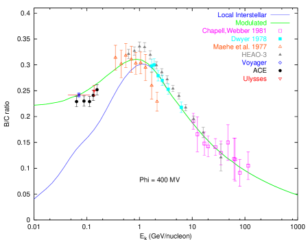
Figure 5: Calculated Boron-to-Carbon ratio compared with observational data. The lower line represents the local interstellar value, while the upper one is the result after solar modulation with $\Phi=400MV$. Observational data: ACE [50], Ulysses [51], Voyager [52], HEAO-3 [53], for others please refer to [54].

In Figure. 5 we show the expected B/C from the propagation model. The propagation model describes the observational data very well. We will use this model to calculate the secondary positron spectrum from cosmic rays fragmentation given in Eq. (9)and the primary positron propagation from DM annihilation given in Eq. (1).

5 Results and Discussion

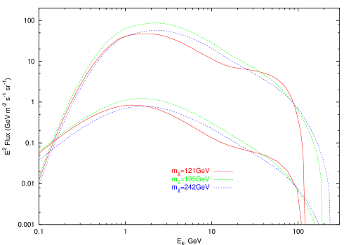
Figure 6: The propagated positron fluxes on the Earth for three neutralino models. Moore profile, containing subhalos with $\gamma=1.7$ and $\rho_{\rm max}=2\times 10^{19}M_{\odot}/kpc^{3}$ is adopted. Upper lines show the local annihilation sources $E^{2}\,Q(E,{\bf r})$ in unit of GeV $m^{-3}s^{-1}$ for the three neutralino models.

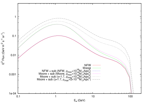
Figure 7: Positron flux on Earth for various DM profiles. The mass of neutralino is $121GeV$.

Once the SUSY model is specified and the contribution from subhalos is taken into account we can incorporate the source term of primary positrons in GALPROP and calculate its spectrum on the Earth. In Figure 6 we show the propagated positron fluxes for three different SUSY models with $m_{\chi}=121,195,242$ GeV. For comparison the local source terms $E^{2}Q(E,{\bf r}={\bf r}_{\odot})$ according to Eq. (1) are also shown. We see that propagation makes the spectra some different from the source spectra. This is because the propagation is energy dependent. The source spectra are somewhat different among the three models because these models lead to different annihilation final states. In the calculation a Moore profile for the smooth component and $\gamma=1.7$ profile for subhalos with $\rho_{\rm max}=2\times 10^{19}M_{\odot}/kpc^{3}$ are adopted.

In Figure 7 we show the positron flux for the $m_{\chi}=121GeV$ model for different DM profiles. It indicates that the fluxes can be different for several times among various DM profiles. The cuspier profiles lead to higher positron fluxes. It should be noted that because of the propagation effects the spectra from different DM profiles are different, although they have the same source spectrum. At lower energy the fluxes have bigger differences, since the low energy positrons have longer propagation distance, and may trace the $\langle\rho^{2}\rangle$ farther away from the Earth. The differences between the NFW (or Moore) profile with and without subhalos are not significant. For subhalos with $\gamma=1.7$ profile the flux is greatly enhanced.

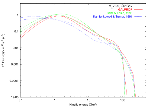
Figure 8: Comparison of positron fluxes of different propagation models.

We then compared the results between GALPROP and other propagation methods. The results are shown in Figure 8. The fluxes for $m_{\chi}=121$ and $242$ GeV based on the Green’s functions given by Kamionkowski & Turner [55] and Baltz & Edsjo [18] are plotted. The BE Green’s function is to solve the diffusive propagation equation analytically and similar to the GALPROP method. However, GALPROP uses realistic astrophysical inputs, and can contain more complex physical process such as reacceleration, while in BE’s method only an average energy loss rate is considered and without convection or reacceleration. After adjusting the propagation parameters to be equivalent, we get similar results between these two models. KT’s result shows a larger difference from these two models. This is comprehensible that the KT Green’s function is acquired by solving the leaky-box equation of propagation with a position-independent source. At low energies the discrepancy is larger because of longer propagation path.

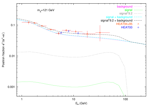
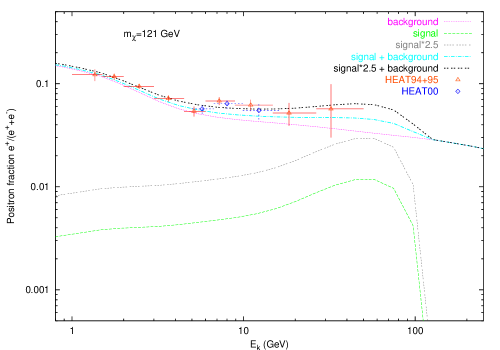
Figure 9: Positron fraction $e^{+}/(e^{+}+e^{-})$ calculated in this work. The left panel shows the result of a Moore DM profile without substructures. The right one is the same as the left but including the subhalos with $\gamma=1.7$ and $\rho_{\rm max}=2\times 10^{19}M_{\odot}/kpc^{3}$. Data points are HEAT measurements in the three fights in 1994, 1995 and 2000 [20, 21].

To give a consistent Galactic positron flux we calculate the background (secondary) positron fraction generated by interaction between primary cosmic-rays and interstellar gas in the same propagation model using GALPROP. In the Figures 9 and 10 we give the background positron fraction. Our results give better description to HEAT data compared with the adapted background fraction in [18, 19, 23, 26]. Therefore the new results requries a smaller “boost factor” to the DM annihilation signals.

Adding the positron flux coming from DM annihilation to the secondary positrons we get the total positron flux. The positron fraction $e^{+}/(e^{+}+e^{-})$ is plotted in Fig. 9 for $m_{\chi}=121$ GeV. We can see from this figure that the expectation reproduces the measurements relatively well if DM subhalos are taken into account. The model with subhalos can contribute several times more than which without subhalos. The best fit to the HEAT data requries “adjustment factor” of $9.2$ and $2.5$ for signals from DM annihilation without and with subhalos respectively.

We don’t think the discrepancy of a factor $2.5$ is serious since there are large uncertainties in calculating the positron fluxes. Firstly there are uncertainties for the positron propagation, as shown in Figure 8. Secondly the random distribution of DM subhalos may have large variance as discussed in [27] since positrons lose energy quickly and have large fluctuations. The variance may lead to large positron flux due to accidence, while in this work we just give the average positron flux. Thirdly we can choose SUSY model which produces more positrons, as shown in Figure 10 for a model with $m_{\chi}=195GeV$. The best fit to HEAT data requries a factor of $1.2$ for this model. It is remarkable that without introducing a large “boost factor” nor the nonthermal production of neutralinos as done in [19] we could explain the HEAT data quite well.

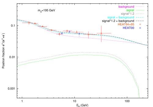
Figure 10: The same as Fig. 9 but for neutralino with mass $m_{\chi}=195GeV$.

It is interesting to notice that at about 8$GeV$, HEAT measurements show some fine structures of the positron fraction, which cannot appear in our calculation. Maybe there are some specific sources or some specific physical process to generate positrons at this energy. However, the errors of the data are too big to give a definite assertion of this property. If it is confirmed by further experiments such as AMS-2, there should be deeper studies about the models we used here.

In summary, in this work we give a consitent and detailed calculation of the Galactic positron flux. We recalculate the background positron flux from cosmic-ray collisions with the interstellar gas in a realistic propagation model GALPROP. The results soft the discrepancy between data and expectations. For the primary positrons from DM annihilation we take the enhancement of subhalos into account. The result shows that the HEAT data can be explained by the two components without introducing “boost factor” or nonthermal production of DM. To account for the excess of positron flux extending subhalo masses to $10^{-6}M_{\odot}$ and requiring a cuspy profile as $\gamma=1.7$ are necessary.

Reference

References

- [1] Jungman G, Kamionkowski M and Griest K, Supersymmetric dark matter, 1996, Phys. Rept. 267 195
- [2] Begeman K G, Broeils A H and Sanders R H, Extended rotation curves of spiral galaxies - dark haloes and modified dynamics, 1991, Mon. Not. R. Astron. Soc. 249 523
- [3] Tyson J A and Fischer P, Measurement of the mass profile of Abell 1689, 1995, Astrophys. J. 446 55
- [4] White S D M, Navarro J F, Evrard A E and Frenk C S, The baryon content of Galaxy clusters - a challenge to cosmological orthodoxy, 1993, Nature 366 429
- [5] Peebles P J E, 1971, Physical Cosmology (Princeton: Princeton University Press)
- [6] Davis M, Efstathiou G, Frenk C S and White S D M, The evolution of large-scale structure in a universe dominated by cold dark matter, 1985, Astrophys. J. 292 371
- [7] Spergel D N, Verde L, Peiris H V et al, First-year Wilkinson Microwave Anisotropy Probe (WMAP) observations: determination of cosmological parameters, 2003, Astrophys. J. Supp. 148 175; Spergel D N et al, Wilkinson Microwave Anisotropy Prob(WMAP) three year results: implications for comology, 2006, Preprint astro-ph/0603449v2
- [8] Bertone G, Hooper D and Silk J, Particle dark matter: evidence, candidates and constraints, 2004, Phys. Rept. 405 279
- [9] Goodman M W and Witten E, Detectability of certain dark-matter candidates, 1985, Phys. Rev. D. 31 3059
- [10] Bottino A, de Alfaro V, Fornengo N et al, On the neutralino as dark matter candidate. II. Direct detection 1994, Astropart. Phys. 2 77
- [11] Bernabei R, Belli P, Montecchia F et al, Searching for WIMPs by the annual modulation signature, 1998, Phys. Lett. B. 424 195
- [12] Bernabei R, Belli P, Montecchia F et al, On a further search for a yearly modulation of the rate in particle Dark Matter direct search, 1999, Phys. Lett. B. 450 448
- [13] Munoz C, Dark matter detection in the light of recent experimental results, 2004, Int. J. Mod. Phys. A 19 3093
- [14] Barger V D, Halzen F, Hooper D et al,Indirect search for neutralino dark matter with high energy neutrinos, 2002, Phys. Rev. D. 65 075022
- [15] Bergstrom L, Edsjo J and Ullio P, Spectral gamma-ray signatures of cosmological dark matter annihilations, 2001, Phys. Rev. Lett.87 251301
- [16] de Boer W, Herold M, Sander C et al, Excess of EGRET Galactic gamma ray data interpreted as dark matter annihilation, 2004, Preprint astro-ph/0408272v2
- [17] Donato F, Fornengo N, Maurin D et al, Antiprotons in cosmic rays from neutralino annihilation, 2004, Phys. Rev. D. 69 063501
- [18] Baltz E A and Edsjo J, Positron propagation and fluxes from neutralino annihilation in the halo, 1999, Phys. Rev. D. 59 023511
- [19] Kane G L, Wang L T and Wang T T, Supersymmetry and the cosmic ray positron excess, 2002, Phys. Lett. B 536 263; Kane G L, Wang L T and Wells J D, Supersymmetry and the positron excess in cosmicrays, 2002, Phys. Rev. D. 65 057701
- [20] Barwick S W, Beatty J J, Bhattacharyya A et al, Measurements of the cosmic-ray positron fraction from 1 to 50 , 1997, Astrophys. J. 482 L191
- [21] Coutu S, Beach A S, Beatty J J et al, Positron measurements with the Heat-pbar instrument, 2001, International Cosmic Ray Conference 1687
- [22] Moskalenko I V and Strong A W, Production and propagation of cosmic-ray positrons and electrons, 1998, Astrophys. J. 493 694
- [23] Baltz E A, Edsjo J, Freese K et al, Cosmic ray positron excess and neutralino dark matter, 2002, Phys. Rev. D. 65 063511
- [24] Hooper D, Taylor J E and Silk J, Can supersymmetry naturally explain the positron excess? 2004, Phys. Rev. D. 69 103509
- [25] Diemand J, Moore B and Stadel J, Earth-mass dark-matter haloes as the first structures in the early Universe, 2005, Nature 433 389
- [26] Cumberbatch D T and Silk J, Local dark matter clumps and the positron excess, 2006, Mon. Not. R. Astron. Soc. 374 455
- [27] Lavalle J, Pochon J, Salati P and Taillet R, Clumpiness of dark matter and positron annihilation signal: computing the odds of the Galactic lottery, 2006, Preprint astro-ph/0603796v2
- [28] Strong A W and Moskalenko I V, Propagation of Cosmic-Ray Nucleons in the Galaxy, 1998, Astrophys. J. 509 212
- [29] Gondolo P, Edsjo J, Bergstrom L et al, DarkSUSY - A numerical package for dark matter calculations in the MSSM, 2000, Preprint astro-ph/0012234v1
- [30] Zhao H S, Analytical models for galactic nuclei, 1996, Mon. Not. R. Astron. Soc. 278 488
- [31] Navarro J F, Frenk C S and White S D M, A universal density profile from hierarchical clustering, 1997, Astrophys. J. 490 493
- [32] Moore B, Governato F, Quinn T et al, Resolving the structure of cold dark matter halos, 1998, Astrophys. J. 499 L5
- [33] Jing Y P and Suto Y, The density profiles of the dark matter halo are not universal, 2000, Astrophys. J. 529 L69; Jing Y P and Suto Y, Triaxial modeling of halo density profiles with high-resolution N-body simulations, Astrophys. J. 574 538
- [34] Reed D, Governato F, Verde J et al, Evolution of the density profiles of dark matter haloes, 2005, Mon. Not. R. Astron. Soc. 357 82
- [35] Bullock J S, Kolatt T S, Sigad Y et al, Profiles of dark haloes: evolution, scatter and environment, 2001, Mon. Not. R. Astron. Soc. 321 559
- [36] Tormen G, Diaferio A & Syer D, Survival of substructure within dark matter haloes, 1998, Mon. Not. R. Astron. Soc. 299 728
- [37] Klypin A, Gottlöber S, Kravtsov A V and Khokhlov A M, Galaxies in N-body simulations: overcoming the overmerging problem, 1999, Astrophys. J. 516 530; Klypin A et al, Where are the missing galactic satellites? 1999, Astrophys. J. 522 82
- [38] Moore B, Ghigna S, Governato F et al, Dark matter substructure within Galactic halos, 1999, Astrophys. J. 524 L19
- [39] Ghigna S, Moore B, Governato F et al, Density profiles and substructures of dark matter halos: converging results at ultra-high numerical resolution, 2000, Astrophys. J. 544 616
- [40] Springel V, White S D M, Tormen G and Kauffmann G, Populating a cluster of galaxies - I. results at , 2001, Mon. Not. R. Astron. Soc. 328 726
- [41] Zentner A R and Bullock J S, Halo substructure and the power spectrum, 2003, Astrophys. J. 598 49
- [42] De Lucia G, Kauffmann G, Springel V et al, Substructures in cold dark matter haoles, 2004, Mon. Not. R. Astron. Soc. 348 333
- [43] Kravtsov A V, Gnedin O Y and Klypin A A, The tumultuous lives of galactic dwarfs and the missing satellites problem, 2004, Astrophys. J. 609 482
- [44] Diemand J, Moore B and Stadel J, Velodicity and spatial biases in cold dark matter subhalo distributions, 2004, Mon. Not. R. Astron. Soc. 352 535
- [45] Gao L, White S D M, Jenkins A, Stoehr F and Springel V, The subhalo populations of CDM dark haloes, 2004, Mon. Not. R. Astron. Soc. 255 819
- [46] Bi X J, Gamma rays from the neutralino dark matter annihilations in the Milky Way substructures, 2006, Nucl. Phys. B. 741 83; Bi X J, Guo Y Q, Hu H B and Zhang X, Detecting the dark matter annihilation at the ground EAS detectors, 2006, Preprint hep-ph/0610387v1
- [47] Berezinsky V S, Gurevich A V and Zybin K P, Distribution of dark matter in the galaxy and the lower limits for the masses of supersymmetric particles, 1992, Phys. Lett. B. 294 221
- [48] Mautin D, Donato F, Tailley R and Salati P, Cosmic rays below in a diffusion model: new constraints on propagation parameters, 2001, Astrophys. J. 555 585
- [49] Moskalenko I V, Strong A W, Ormes J F and Potgieter M S, Secondary antiprotons and propagation of cosmic rays in the Galaxy and heliosphere, 2002, Astrophys. J. 565 280
- [50] Davis A J et al, On the low energy decrease in Galactic cosmic ray secondary/primary ratios, 2000, in AIP Conf. Proc. 528 421
- [51] DuVernois M A, Simpson J A and Thayer M R, Interstellar propagation of cosmic rays: analysis of the ULYSSES promary and secondary elemental abundances, 1996, Astron. Astrophys. 316 555
- [52] Lukasiak A, Voyager measurements of the charge and isotopic composition of cosmic ray Li, Be and B nuclei and implications for their production in the Galaxy, 1999, Proc. 26th Int. Cosmic Ray Conf. 3 41
- [53] Engelmann J J, Ferrando P, Soutoul A, Goret P and Juliusson E, Charge composition and energy spectra of cosmic-ray nuclei for elements from Be to Ni - results from HEAO-3-C2, 1990, Astron. Astrophys. 233 96
- [54] Stephens S A and Streitmatter R E, Cosmic-ray propagation in the Galaxy: techniques and the mean matter traversal, 1998, Astrophys. J. 505 266
- [55] Kamionkowski M and Turner M S, Distinctive positron feature from particle dark-matter annihilations in the galactic halo, 1991, Phys. Rev. D. 43 1774