Recent results from Yakutsk experiment: development of EAS, energy spectrum and primary particle mass composition in the energy region of $10^{15}-10^{19}$ eV

Abstract

Experimental data obtained at the Yakutsk array after the modernization in 1993 are analyzed. The characteristics of EAS longitudinal and radial development found from the charged particle flux and EAS Čerenkov light registered at the Yakutsk complex array are presented. The energy spectrum of EAS obtained from Čerenkov light and an estimate of the PCR mass composition are presented.

I INTRODUCTION

The measurements of charged particles (electrons and muons with $E_{\text{th}}\geq 1\cdot\sec{\theta}$ GeV) and Čerenkov EAS radiation are carried out at the Yakutsk EAS array during more than 35 years. After the modernization in 1993 b:1 , the Yakutsk array significantly improves the measurement accuracy of main EAS characteristics and increases a temp of statistics set in the energy range of $10^{17}-5\cdot 10^{18}$ eV. It has come about through the increase of the number of measurement stations and the decrease of separation between them.

A spectrum of energy, dissipated by primary cosmic rays (PCR) in extensive air showers (EAS), have been obtained from these data and estimation of PCR mass composition was made b:2 ; b:3 . Another method for estimation of primary particles mass composition will be presented hereinafter.

There is a perspective method for analysis of primary cosmic rays (PCR) chemical composition based on conjoined analysis of longitudinal (cascade curve) and lateral (structural functions of electron, muon and Čerenkov components) development of EAS. With such a complex approach to measurement of shower characteristics here we have an opportunity of full reconstruction of PCR mass composition using specific mathematical techniques, for instance, inverse problem solving method b:4 ; b:5 ; b:6 , simplex method b:7 and so on.

II LATERAL DISTRIBUTION OF DIFFERENT EAS COMPONENTS

II.1 Charged particles

Fig. 1 shows the average lateral distribution functions (LDF) of charged particles for $E_{0}\sim 10^{15}-10^{19}$ eV constructed by the method used for the Yakutsk array b:9 . From fig. 1 it follows that at $E_{0}\sim 10^{15}-10^{17}$ eV LDF’s are well measured in the distance interval of $15-400$ m from a shower core, whereas at $E_{0}\geq 10^{17}$ eV they are only measured in the distance interval of $50-1300$ m. The curves are the approximation $\rho(R)$ by the function (1) from the work b:10 :

$$\rho(R)=\frac{N_{\text{s}}}{2\pi R^{2}_{\text{m.s}}}\cdot\left(\frac{r}{R_{\text{m.s.}}}\right)^{-1.2}\times\left(1+\frac{r}{R_{\text{m.s.}}}\right)^{-3.33}\cdot\left[1+\left(\frac{r}{10R_{\text{m.s.}}}\right)^{2}\right]^{-0,6}\text{,}$$ (1)

where $N_{\text{s}}$ is the total number of charged particles at observation level, $R_{\text{m.s.}}$ is a mean square radius of LDF of charged particles. It is seen from fig. 3, 4 that the function (1) describes well experimental data both at $E_{0}\sim 10^{15}-10^{17}$ eV and in the showers at $E_{0}\geq 10^{17}$ eV.

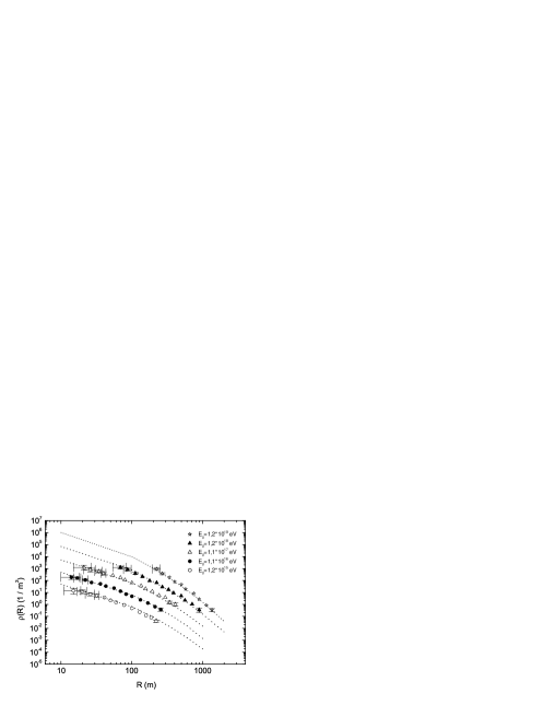
Figure 1: Average LDFs of charged particles measured at the Yakutsk EAS complex array.

Figure 2: Lateral distributions of charged particles and muons. Circles are data from the Yakutsk experiment. Curves — from QGSJET model calculations for the showers generated by the primary proton.

Thus, the function (1) can be used to determine $N_{\text{s}}$ in the showers at the highest energies where there are no measurements of particle density at small distances.

On fig. 2 a comparison is presented between the lateral distributions of charged particles and muons with $E_{\text{th}}\geq 1$ GeV and calculation result from work b:11 . In the work b:11 , a hybrid scheme of EAS simulation is used together with QGSJET01 model. As it follows from fig. 2, calculations give more slope function as for charged particles, so for muons at distances more than $600$ m from the shower axis. If calculated value of $\rho(600)$ (QGSJET01 model) is used for shower energy estimation together with model-independent method for energy estimation used in Yakutsk experiment b:12 then the energy estimated with QGSJET01 would be underestimated by the value equal to the difference of densities $\rho(600)$ (see fig. 2).

II.2 Čerenkov light

Čerenkov light measurements at the Yakutsk array last for more than 35 years. Since the year 1993 there are 50 operating Čerenkov detectors with receiving area of photocathode $176$ and $530$ cm². Observation results for last years are presented on fig. 3. On the same figure calculations are shown from the work b:13 (Dedenko et al.) for primary proton and zenith angle $\theta=0^{\circ}$. In the work a 5-level scheme for air shower generation is used. One can see a good correspondence in experimental data at medium and large distances from the axis. At distances $<80$ m measured flux of Čerenkov light is less than one following from calculations. This discrepancy could be explained as with distinct mass composition so with different zenith angle. Experimental LDFs of Čerenkov light are given for $\theta=17-18^{\circ}$.

On fig. 4 our results (circles) are given in comparison with the data obtained by Haverah Park group b:14 . The solid line is calculation from work b:15 . There is a good correspondence with the experimental data.

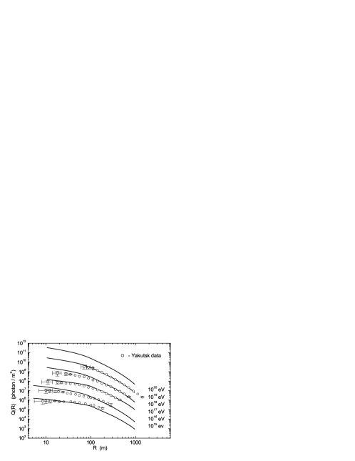
Figure 3: The lateral distribution of EAS Čerenkov light. Curves — QGSJET (Dedenko et al.).

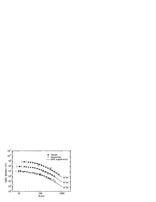
Figure 4: Comparison between the data from Yakutsk and Haverah Park. Curves — QGS (Lagutin et al.).

III LONGITUDINAL DEVELOPMENT OF EAS

Longitudinal development of high- and ultra-high energy air showers was reconstructed from Čerenkov light registered at the Yakutsk EAS array. For this purpose a method proposed in work b:6 was used. Results of the reconstruction are shown on fig. 5 in comparison with calculations obtained for different hadron interaction models. Calculations have been performed for primary protons and iron nuclei. Experimental data presented on fig. 5 are well described by models with fast development like QGSJET in case of primary proton. It can be concluded that primary mass composition is a mixture of nuclei with varying portion of heavy nuclei. The most significant change is observed in the energy region of $10^{16}-10^{17}$ eV (experimental data tend towards heavy composition) and above $3\cdot 10^{18}$ eV where mass composition is closer to proton.

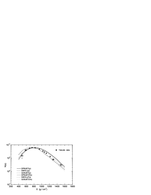
Figure 5: Average cascade curve of the shower development at $E_{0}=10^{19}$ eV. Curves — different hadronic model calculations.

IV EMPIRICAL ESTIMATE OF EAS ENERGY AT THE YAKUTSK ARRAY

The primary energy of a shower at the Yakutsk EAS array is calculated with the expression

$$E_{0}=E_{\text{ei}}+E_{\text{el}}+E_{\mu}+E_{\text{hi}}+E_{\mu\text{i}}+E_{\nu}\text{.}$$

The energy scattered by electrons in the atmosphere above the observation level is given by the expression

$$E_{\text{ei}}=k(X,P_{\lambda})\cdot F\text{,}$$

Here, $F$ is total flux of Čerenkov light from the EAS and $k(X,P_{\lambda})$ — is the coupling coefficient that represents the transparency of the real atmosphere and character of the longitudinal shower development, where $P_{\lambda}$ is spectral atmosphere transparency (SAT), calculated during lidar measurements.

The energy of electrons at the observation level is calculated as

$$E_{\text{el}}=2.2\cdot 10^{6}\cdot N_{\text{s}}(X_{0})\cdot\lambda_{\text{eff}}\text{,}$$

where $N_{\text{s}}(X_{0})$ is the total number of charged particles at sea level and $\lambda_{\text{eff}}$ is the absorption mean free path of shower particles obtained from the correlation of the parameters $N_{\text{s}}(X_{0})$ and $Q(R=400)$ at different zenith angles. Other components are: $E_{\mu}=\varepsilon_{\mu}\cdot N_{\mu}$; $E_{\mu\text{i}}=(0.12\pm 0.09)\cdot E_{\mu}$; $E_{\text{hi}}=(5.6\pm 2.2)\cdot E_{\mu}$; $E_{\nu}=(0.64\pm 0.18)\cdot E_{\mu}$.

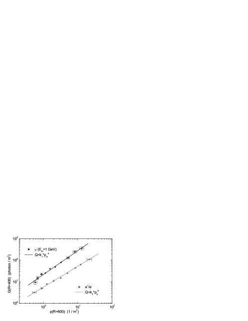
Figure 6: Estimation of the EAS energy by density $\rho_{\text{s}}(600)$, $\rho_{\mu}(600)$ and $Q(400)$.

Using experimental data presented on fig. 6, the following expressions have been obtained at the Yakutsk array for energy estimation by density of charged particles and muons with $E_{\text{th}}\geq 1$ GeV:

$$\lg{E_{0}} = 17.68+0.98\cdot\lg{\rho_{\text{s}}(600)}$$ (2)

$$\lg{E_{0}} = 18.32+1.12\cdot\lg{\rho_{\mu}(600)}$$ (3)

V ENERGY SPECTRUM IN THE ENERGY REGION OF $\sim 10^{15}-10^{20}$ eV

In addition to charged particle surface detection, there is another technique used at the Yakutsk array — the air Čerenkov light measurement, which can be used to draw out the cosmic ray spectrum in independent way b:16 . The spectrum covers wide energy region $10^{15}-10^{20}$ eV. On fig. 7, fig. 8 Čerenkov spectra are compared to calculations with different models of cosmic ray propagation in the Universe b:17 ; b:18 . It follows from fig. 7 and fig. 8 that galactic model describes well our spectrum in the region of $10^{15}-10^{18}$ eV b:17 and metagalactic model b:18  — above $10^{18}$ eV. As it is seen from fig. 8, in the region of $10^{17}-10^{18}$ eV a boundary of transition from galactic cosmic rays to metagalactic possibly exists. This hypothesis requires further research.

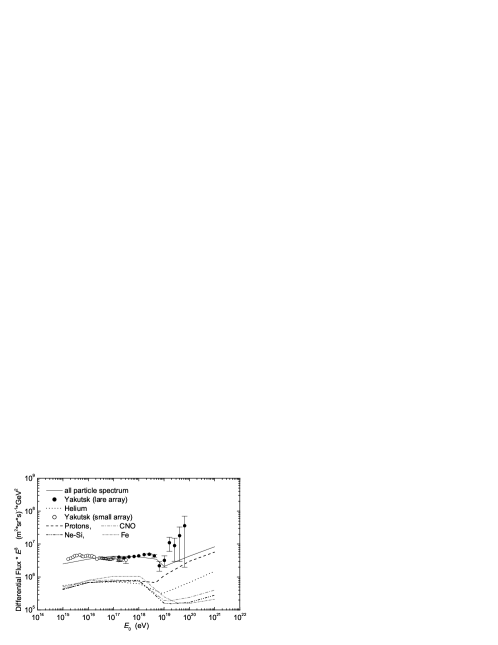
Figure 7: Spectra measured in Yakutsk using the air Čerenkov light. Curves are results of anomalous diffusion model calculations b:17 .

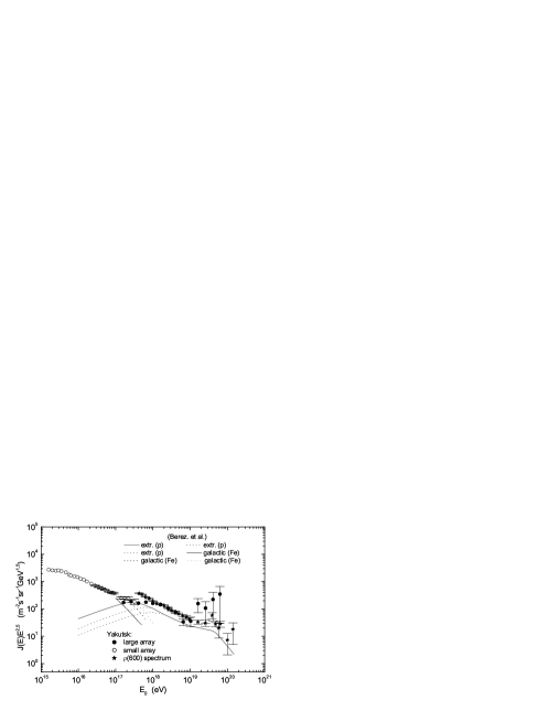
Figure 8: Calculated spectrum of extragalactic proton (solid curve) and of galactic iron spectra (dotted curves) b:18 compared to all-particle spectrum from Yakutsk array.

VI MASS COMPOSITION OF PRIMARY COSMIC RAYS

To interpret Yakutsk experimental data a set of $X_{\text{max}}$ and $\rho_{\text{s}}(600)$ calculated values obtained with CORSIKA simulation code (v.6.0, QGSJET model) was used. Calculations were carried for five primary nuclei (p, He, C, Si, Fe) at three primary energy values $10^{17}$, $10^{18}$, $10^{19}$ eV b:19 . In the work, two-dimensional probability densities $F(X_{\text{max}},\rho(600))$ were used with preliminary procedure of standardization of the experimental data over the whole $(X_{\text{max}},\rho_{\text{s}}(600))$ data set. In the numerical implementation of this method, variables $\tau$ and $\rho$ were used instead of $(X_{\text{max}},\rho_{\text{s}}(600))$:

$$\tau=\frac{X_{\text{max}}}{\sigma_{\text{x}}}-\left<\frac{X_{\text{max}}}{\sigma_{\text{x}}}\right>$$ (4)

$$\rho=\frac{\lg{\rho(600)}}{\sigma_{\lg{\rho(600)}}}-\left<\frac{\lg{\rho(600)}}{\sigma_{\lg{\rho(600)}}}\right>,$$ (5)

where $\sigma_{\text{i}}$ — is a mean square error.

For each of considered energy value and kind of primary nuclei (including nuclei joint in groups $\text{p}+\text{He}$, C, $\text{Si}+\text{Fe}$) probability distributions densities $f(\tau,\rho)$ were constructed. The intersection of $f(\tau,\rho)$ surfaces gives lines $m_{1}$ and $m_{2}$ which optimally divide nuclei into ($\text{p}+\text{He}$), C and ($\text{Si}+\text{Fe}$) groups respectively. The simulations showed that with dividing of data into three groups, the effectiveness of nuclei group ($\text{p}+\text{He}$) to fall into the zone 1 and of ($\text{Si}+\text{Fe}$) to fall into the zone 3 is up to $90$ %. In the zone 2 a strong mixing between showers from different primaries occurs and a portion of carbon is $\sim 50$ % from all particles in this zone.

The $X_{\text{max}}$ value characterizes a maximum of cascade development in individual shower and $\rho(600)$ is the density of particles at the observational level.

Fig. 9 presents the results of multicomponent analysis of $(X_{\text{max}},\rho(600))$ data set obtained at the Yakutsk EAS array. It is seen that there is a correlation between the observed maximum of shower development and the density of charged particles

The analysis was carried out for three values of energy, $2.4\cdot 10^{17}$, $9.8\cdot 10^{17}$ and $4.8\cdot 10^{18}$ eV. In this notion, the point cloud represents standardized values, whose location regions characterize zones directly connected with the mass number of a primary particle. Lines represent borders of such zones. In this case, lines $m_{1}$ and $m_{2}$ optimally divide nuclei into groups ($\text{p}+\text{He}$), C and ($\text{Si}+\text{Fe}$). One can see from fig. 9, that the points are distributed over the zones non-uniformly.

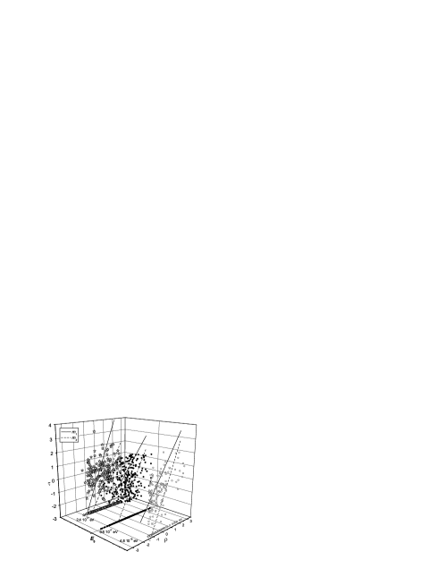
Figure 9: Standardized $X_{\text{max}}$ and $\rho_{600}$ experimental data at different energy values. $m_{1}$ is a borderline between nuclear groups ($\text{p}+\text{He}$) and C, $m_{2}$ is a borderline between nuclear groups C and ($\text{Si}+\text{Fe}$).

Distribution of statistics over the energy intervals draws attention. The portion of ($\text{p}+\text{He}$) nuclei increases from $50$ % to $53$ % and a portion of carbon nuclei — from $23$ % to $31$ %. At the same time, the portion of heavy nuclei decreases from $27$ % to $16$ % with growth of energy from $2.4\cdot 10^{17}$ eV to $4.8\cdot 10^{18}$ eV. The error to recognize the nuclei for the energies of $10^{17}-10^{19}$ eV does not exceed 30 %. Such a distribution of nuclei in PCR does not contradict the conclusions about increase of the portion of protons and helium nuclei in the limit energy region made in our earlier works b:20 ; b:21 ; b:22 where other methods were used.

On fig. 10 a portion of light, medium and heavy nuclei obtained in our analysis is shown. It is seen from the figure that at $E_{0}\geq 4\cdot 10^{18}$ eV portion of heavy nuclei decreases. From fig. 11 it follows that in the energy region $10^{16}-10^{17}$ eV $\left<\ln{A}\right>$ value has its maximum value and after $5\cdot 10^{17}$ eV starts decreasing. Such a change in mass composition in the energy region of $10^{16}-10^{17}$ eV might be caused by modernized diffusion mechanism of cosmic rays propagation in the Galaxy b:17 and possible influence upon the spectrum by lighter extragalactic component arriving from beyond the Galaxy b:18 .

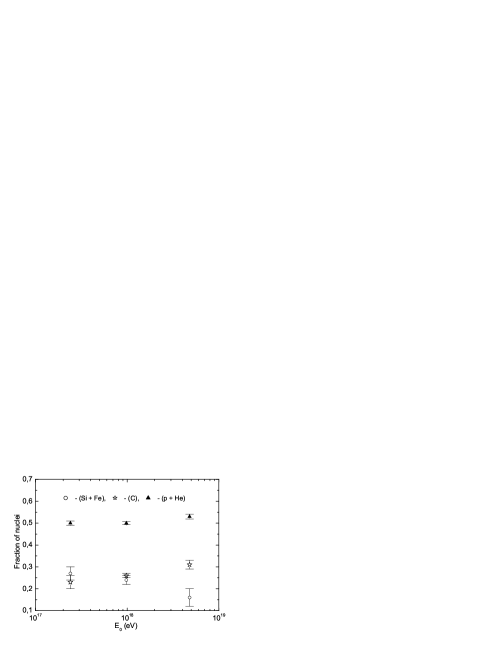
Figure 10: Fraction of the different nuclei in the energy range $E_{0}=10^{17}-10^{19}$ eV.

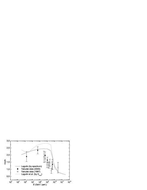
Figure 11: Mean mass numbers in cosmic rays of high- and ultra-high energies. Curves — calculations from anomalous diffusion model of cosmic rays propagation (Lagutin et al. 2004).

- (1) V. P. Artamonov, B. N. Afanasiev, and A. V. Glushkov. Izv. RAN, 58(12):92–97, 1994. (in Russian).
- (2) A. A. Ivanov, S. P. Knurenko, and I. Ye. Sleptsov. In Nucl. Phys. B (Proc. Suppl.), number 122, pages 226–230, 2003.
- (3) S. P. Knurenko, V. P. Egorova, and A. A. Ivanov et al. In Nucl. Phys. B (Proc. Suppl.), number 151, pages 92–95, 2006.
- (4) S. I. Nikolsky, V. P. Pavlyuchenko, and Yi. N. Stamenov. In Kratkiye soobsheniya po fizike, number 9, pages 49–55. M.: FIAN, 1981. (in Russian).
- (5) M. N. Dyakonov, A. A. Ivanov, and S. P. Knurenko. In Cosmic rays with the energy above eV, pages 34–47. Yakutsk: YF SO AN SSSR, 1983. (in Russian).
- (6) S. P. Knurenko, V. A. Kolosov, and Z. E. Petrov et al. In Proc. 27th ICRC, Hamburg, volume 1, pages 157–160, 2001.
- (7) A. A. Ivanov, I. Ye. Sleptsov, and S. P. Knurenko. Izv. RAN, 69(3):363–365, 2005. (in Russian).
- (8) M. N. Dyakonov, V. P. Egorova, and A. A. Ivanov et al. In Ultra-high energy cosmic rays, pages 15–33. Ya. F. SO AN SSSR, 1979. (in Russian).
- (9) A. A. Lagutin, R. I. Raikin, N. Inoue, and A. Misaki. Journ. Phys., 28(6):1259–1274, 2002.
- (10) H. J. Drescher. In Nucl. Phys. B (Proc. Suppl.), number 151, pages 151–158, 2005.
- (11) S. P. Knurenko, A. A. Ivanov, and I. Ye. Sleptsov. JETP Letters, 83(11):473–477, 2006.
- (12) L. G. Dedenko, G. F. Fedorova, and V. I. Galkin et al. In Proc. 29th ICRC, Pune, volume 8, page 308, 2005.
- (13) R. T. Hammond et al. In Proc. 15th ICRC, Plovdiv, volume 8, page 308, 1977.
- (14) A. A. Lagutin et al. Number 1289. Leningrad, June, 1987. Preprint.
- (15) S. P. Knurenko, V. A. Kolosov, and Z. E. Petrov et al. In Proc. 27th ICRC, Hamburg, volume 1, pages 145–147, 2001.
- (16) A. A. Lagutin et al. In Nucl. Phys. B (Proc. Suppl.), number 97, page 267, 2001.
- (17) V. Berezinsky et al. astro-ph/0302483.
- (18) A. A. Lagutin and N. V. Stanovkina. Izv. AGU, (5):76–79, 2004. (in Russian).
- (19) M. N. Dyakonov, V. P. Egorova, and S. P. Knurenko et al. In Extensive air showers with energy above eV, pages 29–56. Ya. F. SO AN SSSR, 1987. (in Russian).
- (20) M. N. Dyakonov, V. P. Egorova, and A. A Ivanov i dr. Pisma v ZhETF, 50(10):408–410, 1989. (in Russian).
- (21) M. N. Dyakonov, S. P. Knurenko, and V. A. Kolosov i dr. In Modern problems of gravity. Trudy Vsesoyuznogo soveshchaniya., pages 114–126. Yakutsk, 1990. (in Russian).