Synthetic Observations of Carbon Lines of Turbulent Flows
in Diffuse Multiphase Interstellar Medium

Abstract

We examine observational characteristics of multi-phase turbulent flows in the diffuse interstellar medium (ISM) using a synthetic radiation field of atomic and molecular lines. We consider the multi-phase ISM which is formed by thermal instability under the irradiation of UV photons with moderate visual extinction $A_{V}\sim 1$. Radiation field maps of C⁺, C⁰, and CO line emissions were generated by calculating the non-local thermodynamic equilibrium (nonLTE) level populations from the results of high resolution hydrodynamic simulations of diffuse ISM models. By analyzing synthetic radiation field of carbon lines of [C II] 158 $\mu$m, [C I] ${}^{3}P_{2}-^{3}P_{1}$ (809 GHz), ${}^{3}P_{1}-^{3}P_{0}$ (492 GHz), and CO rotational transitions, we found a high ratio between the lines of high- and low-excitation energies in the diffuse multi-phase interstellar medium. This shows that simultaneous observations of the lines of warm- and cold-gas tracers will be useful in examining the thermal structure, and hence the origin of diffuse interstellar clouds.

1 Introduction

Recent studies of the multi-phase interstellar medium (ISM) have demonstrated that the origin of small scale interstellar turbulence might be attributed to the thermally unstable nature of the ISM itself (Koyama & Inutsuka, 2002, 2006; Kritsuk & Norman, 2002a, b; Audit & Hennebelle, 2005; Heitsch et al., 2005; Inutsuka, Koyama & Inoue, 2005; Vazquez-Semadeni et al., 2006). Until recently, most theoretical work on interstellar turbulence has assumed that the ISM is isothermal (see for recent reviews, Mac Low & Klessen 2004; Elmegreen & Scalo 2004, and references therein). This approximation has been imposed mainly because quiescent gas evolves almost isothermally at 10K as a result of the thermal balance between radiative heating and dust emission cooling where external UV radiation is well-shielded (Hattori, Nakano & Hayashi, 1969), and partly because of limited computational ability. Detailed analyses of the one-dimensional collapse due to thermal instability can be found in, for example, Hennebelle & Pérault (1999, 2000) and Koyama & Inutsuka (2000). The situation has changed since Koyama & Inutsuka (2002) first pointed out that the thermally unstable nature of multi-phase ISM is able to maintain the turbulent flows. Since then, various attempts have been made to examine the properties of the multi-phase turbulent ISM (Koyama & Inutsuka, 2002; Kritsuk & Norman, 2002a, b; Audit & Hennebelle, 2005). Koyama & Inutsuka (2002) performed two-dimensional simulation of a supernova-induced shock propagating into warm ($\sim$ 6000K) ISM. They demonstrated that broad emission linewidths can be generated in the post-shock layer, where chaotic structures are formed by thermal instability. In their calculation, tiny, cold and dense clumps were seen to move in the surrounding warm diffuse medium subsonically with respect to the warm medium, but supersonically to the sound speed in the cold clumps. In this article, we refer to this model as the “two-phase model” where two thermal states, i.e., cold clumps and warm medium, are generated by thermal instability. Similar conclusions have also been reached by other authors. Among them, Kritsuk & Norman (2002a, b) performed three dimensional simulations of a multi-phase medium and examined the evolution of kinetic energy of the resulting turbulence. Audit & Hennebelle (2005) simulated a two-dimensional converging flow, where the post-shock thermally unstable gas is continuously provided by the two shock waves that confine the post-shock gas. They showed that complex structures similar to those of Koyama & Inutsuka (2002) are formed, and discussed their evolution by comparing cooling length, fragment scale of the cold neutral medium (CNM), Field length, and the typical size of the shocked layer. Heitsch et al. (2005) and Vazquez-Semadeni et al. (2006) have followed this line of work and discussed the observational signature as well. While the calculations above focus mainly on neutral atomic gas, Pavlovski et al. (2005) examined molecular gas of much higher density ($n_{\rm H}\simeq 10^{6}$ cm^-3). They concluded that the gas is kept isothermal due to the fast reformation of the coolant molecules behind shock waves in the dense molecular clouds.

In this article, we concentrate on more diffuse gas ($\approx 1$ cm^-3), which is warmed by mild UV photoelectric heating, and focus on observational characteristics of the two-phase medium. Emission-line diagnosis of atomic and molecular radiation in millimeter and submillimeter bands provides a powerful tool for observational study of interstellar turbulence (e.g., Padoan et al., 2001; Bergin et al., 2004). In addition to existing telescopes equipped with submillimeter receivers, such as SubMillimeter Array (SMA) and Atacama Submillimeter TElescope (ASTE), the highly sensitive instruments of Atacama Large Millimeter/submillimeter Array (ALMA) will be available before long. We thus examine how a characteristic feature of the two-phase turbulence model should appear in observational quantities. We try to find and propose unambiguous and robust observational indicators for the two-phase turbulence model. For this purpose, we perform hydrodynamical simulations of two-phase turbulent flows, and then calculate line emission of atomic carbons and CO molecules. Based on the synthetic emission maps, our results are more suitable for direct comparison with observation than the density or temperature distributions, which are provided by previous hydrodynamical simulations.

The organization of this article is as follows: In §2 we describe our model and basic equations. In §3 we display our synthetic radiation maps of the two-phase model as well as the conventional one-phase (isothermal) turbulent flow model. We also show the results of the analyses of our simulated emission maps of C⁺, C⁰, and CO lines. In §4 we discuss the limits of and uncertainty about our calculation and discuss its relevance to current observational results. We summarize this article in the final section (§5).

2 Models and Calculations

We consider diffuse clouds irradiated by mild UV background radiation of $G_{0}=1$ (where $G_{0}$ is the typical interstellar UV strength in Habing unit), which is attenuated with average visual extinction $A_{V}\lesssim$ 0.1. We perform hydrodynamical simulations first, and then calculate line-emissivity distributions using the simulation data. In the following, we present equations and assumptions for hydrodynamical and radiation calculations in this order.

2.1 Hydrodynamic Equations

We solve an ordinary set of hydrodynamical equations:

$$\frac{\partial\rho}{\partial t}+\nabla\cdot(\rho\boldmath{v}) = 0,$$ (1a)

$$\frac{\partial\boldmath{v}}{\partial t}+(\boldmath{v}\cdot\nabla)\boldmath{v} = -\frac{\nabla P}{\rho},$$ (1b)

$$\frac{\partial\rho e}{\partial t}+\nabla\cdot(\rho e\boldmath{v})+P\nabla\cdot\boldmath{v} = \frac{\rho}{m_{H}}\Gamma-\left(\frac{\rho}{m_{H}}\right)^{2}\Lambda(T)$$ (1c)

$$+\nabla\cdot(K\nabla T)$$

where $\rho$ is the density, $P$ is the pressure, $e=P/(\gamma-1)$ is the specific internal energy with the adiabatic index $\gamma=5/3$, $\Gamma$ and $\Lambda$ represent the heating and cooling rates, respectively, and $\boldmath{v}$ is the velocity of a fluid element. The last term of the third equation (1c) represents thermal conduction. The thermal conduction coefficient $K=2.5\times 10^{3}T^{1/2}$ ergs cm^-1 K^-1 sec^-1 is taken from Parker (1953), which is valid for temperature $T\lesssim 4.47\times 10^{4}$K. For cooling and heating rates, we employ the fitting formulae shown by equation (8) of Koyama & Inutsuka (2006). The formulae are derived by approximately describing the result of Koyama & Inutsuka (2000), who performed non-equilibrium thermal calculations of one-dimensional shock waves. Their formulae contain dust-grain photoelectric heating, cosmic ray and X-ray ionization heating, H₂ formation and destruction, and line cooling by atomic and molecular emission. In equation (1b) we do not introduce the physical viscosity, which affects the saturation level of turbulent motions, because we are more interested in characteristic features in radiation field rather than detailed arguments on the mechanism for maintaining the turbulent motion. Detailed systematic analyses of the saturation amplitude of two-phase turbulent motions are found in Koyama & Inutsuka (2006). We can safely ignore back reactions by cooling radiation to hydrodynamical evolutions either via radiation pressure or radiation force.

Our two-dimensional simulations employ a scheme based on the second-order Godunov method. In order to correctly resolve thermal conduction-induced structures, the Field length $\lambda_{\mathrm{F}}=(KT/n^{2}\Lambda)^{1/2}$, which is the characteristic length scale of thermal conduction, must be resolved by more than three cells (the so-called Field condition, after Koyama & Inutsuka, 2004). Our calculations satisfy this condition with the number of Eulerian grids 2048² in the simulation box of 2.4$\times$2.4 pc².

We introduce a supersonic velocity field to the medium of initially uniform density and temperature, and calculate its evolution without an external driving force (i.e., so-called decaying turbulence). The initial supersonic velocity field has an average Mach number of $\langle\mathcal{M}\rangle\approx 10$, and power spectrum $P(k)\propto k^{-6}$ in the range of $1\leq k/2\pi=1/\lambda\leq 4$, in units of the reciprocal of the size of the simulation box $\lambda$. The purpose of this paper is to simulate the radio band observation of certain samples of turbulent clouds. Thus we set up the initial conditions rather arbitrarily and calculate the dynamical evolution of the relaxation process from these highly turbulent flows. For the actual simulation of the observation described below, we choose snapshots of the time evolution that would mimic the observed velocity profiles (i.e., position-velocity diagram) of diffuse clouds.

2.2 Method of Radiation Calculation

We solve non-local thermodynamic equilibrium (nonLTE) level populations for relevant lines of atomic and molecular carbon, C⁺, C⁰, and CO. Each level population is determined by solving the equations of detailed balance for transitions as a function of local density and temperature taken from the hydrodynamical calculations. In our model of mildly UV-irradiated diffuse medium, in addition to the Ly$\alpha$ line of atomic hydrogen in the UV band, various millimeter and submillimeter lines contribute to the cooling. Among the line-cooling processes, the contribution of [C II] fine structure cooling is dominant in a wide density range of diffuse regimes (see Figure 1a of Koyama & Inutsuka, 2000). Toward higher density, the role of C⁰ and CO cooling gradually increases. Around the column density $N_{\rm H}=10^{20}$cm^-2 where background UV radiation of $G_{0}=1$ begins to be shielded, the dominant coolant changes from ionic to molecular carbon. Our ISM model, which includes heating and cooling under $N_{H}=10^{20}$cm^-2, corresponds to the atomic/molecular transition region, and thus ionic, neutral and molecular carbon species should exist simultaneously. Therefore we examine three species of carbon, i.e., C⁺, C⁰, and CO, in order to probe various thermal states in multi-phase ISM. We calculate C II and C I fine structure transitions, whose excitation energies are 92K([C II]), 24K([C I]${}^{3}P_{1}-^{3}P_{0}$), 39K([C I]${}^{3}P_{2}-^{3}P_{1}$), and 63K([C I]${}^{3}P_{2}-^{3}P_{0}$), as well as CO($J-$($J-1$)) rotational transitions, with $5.5J$ K, where $J$ is the rotational quantum number.

For [C II] 158$\mu$m line, we use a modified cooling function by Koyama & Inutsuka (2002);

$$\Lambda_{\mathrm{CII}} = 2.8\times 10^{-28}\sqrt{T}\cdot\exp\left(-\frac{92}{T}\right)$$ (2)

$$\times y(\mathrm{C}^{+})[y({\mathrm{H}}^{0})+y({\mathrm{H}_{2}})]{n_{\rm H}}^{2}$$

$$~{}~{}~{}~{}~{}~{}\mathrm{erg}~{}\mathrm{sec}^{-1}\mathrm{cm}^{-3},$$

where $y(X)=n(X)/n_{\rm H}$ represents the fractional abundance of the line-emitting particle $X$. Both atomic and molecular hydrogen work as collision partners for exciting C⁺. In the regime where C II cooling dominates, we can safely replace the term for collision partners with $y({\mathrm{H}}^{0})+y({\mathrm{H}_{2}})=y({\mathrm{H}}^{0})$.

The emissivities per unit volume by [C I] and CO lines are calculated by solving the nonLTE level population. The emissivity of species $X$ by transition from level $i$ to $j$ per unit volume (cooling rate) is given by

$$\Lambda_{X,ij}=h\nu_{ij}A_{ij}n(X,i),$$ (3)

where $h\nu_{ij}$ is the energy difference between levels $i$ and $j$, $A_{ij}$ is the Einstein A-coefficient for spontaneous emission from energy level $i$ to $j$, and $n(X,i)$ is the population density of species $X$ and energy level $i$. The level populations are obtained by solving the equations of statistical balance:

$$n(X,i)\sum_{j^{\prime}}(A_{ij^{\prime}}+C_{ij^{\prime}})=\sum_{j^{\prime}}n(X,j^{\prime})[A_{j^{\prime}i}+C_{j^{\prime}i}].$$ (4)

In the above equation, $C_{ij}$ is the collisional transition rate per emitting particle, which is written with the collisional rate coefficient $\gamma_{ij}$ as

$$C_{ij}=\sum_{Y}n(Y)\gamma_{ij},$$ (5)

where $n(Y)$ indicates the density of collision partner $Y$. For neutral carbon atoms, we consider the triplet in the electronic ground state (${}^{3}P_{0},^{3}P_{1},^{3}P_{2}$). Relevant transition coefficients are taken from Hollenbach & McKee (1989). The collision partners for excitation of atomic carbon include atomic hydrogen and electron, and neglect H₂ for only a small contribution of H₂ is expected where C I abundance and line emission have their peaks (the abundance of C⁰ reaches its maximum between the surface of UV irradiated region and the well-shielded inner region where most of carbon is locked in CO molecules). For CO molecules, we make use of a simplified formula for the collisional rate coefficients of McKee et al. (1982). CO is assumed to be excited by collision with atomic and molecular hydrogen. We use the same collisional coefficient as atomic hydrogen for H₂.

In order to calculate line intensities we need to know the ionization degree and the chemical abundances for each species. This requires non-equilibrium calculation of chemical evolution along with hydrodynamical simulation, which is computationally very expensive. To avoid this difficulty, here we simply assume uniform abundance distribution, and a prescribed variation in terms of temperature (see §4.1). For the ionization degree, we assume an electron fraction of $y(e)=10^{-2}$ referring to the thermal equilibrium abundances of Wolfire et al. (1995). In the neutral medium we are considering, change in the assumed value of $y(e)$ does not significantly alter the results since the collisional transition by electrons is not dominant. For carbon species, we take $y({\mathrm{C}^{+}})=10^{-3}$ and $y({\mathrm{C}^{0}})=y(\mathrm{CO})=3\times 10^{-7}$. These abundances are taken from typical values in the one-dimensional calculation of Koyama & Inutsuka (2000) except for ${\mathrm{C}^{0}}$. The abundance of ${\mathrm{C}^{0}}$ was not calculated in Koyama & Inutsuka (2000), and we arbitrarily assumed the same value as CO for simplicity. The fractions of C⁰ and CO are affected by such factors as the degree of shielding of ultraviolet radiation and the abundances of other species. We try to derive quantities that are independent of the abundance distribution, and defer discussion on the effects of chemical evolution in our model to later in §4.1.

Line emissivity of each fluid element has the thermally broadened profile

$$\phi(\nu)=\frac{1}{\Delta\nu_{D}\sqrt{\pi}}\exp\left(-\frac{(\nu-\nu_{0})^{2}}{(\Delta\nu_{D})^{2}}\right),$$ (6)

where $\nu_{0}$ denotes the frequency of the line center, and $\Delta\nu_{D}=(\nu_{0}/c)\sqrt{2k_{B}T/m}$ denotes the thermal width at temperature $T$. Line profiles are obtained by convolving the thermal broadening with the line centroid $\nu_{0}$ Doppler-shifted by the bulk fluid motion. The bulk fluid velocity is taken from results of the hydrodynamical calculations.

3 Results

3.1 Line Emission Maps

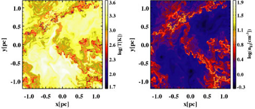
Figure 1: (a) Temperature and (b) density distributions of the two-phase flow model at time $t=2.479$ Myr. Numerous tiny dense and cold clumps are formed within the simulation box.

Figure 1 shows a snapshot of temperature and density distributions. In the density distribution map (Figure 1b), numerous tiny dense clumps are observed, having been formed as a consequence of phase transition in the thermally unstable medium after the initial shock heating. Comparing Figures 1a and b, we can easily recognize that the density map is just a color-inverted version of the temperature map. This is due to the fact that this turbulent flow is essentially driven by the thermal instability characterized by its approximate isobaricity. Under almost uniform pressure, thermally unstable gas forms numerous tiny cold and dense clumps within the surrounding warm and diffuse gas (Koyama & Inutsuka, 2002; Kritsuk & Norman, 2002a; Audit & Hennebelle, 2005). Figures 2a and 2b represent the synthesized emissivity maps of [C II] 158 $\mu$m and CO$(1-0)$ lines.

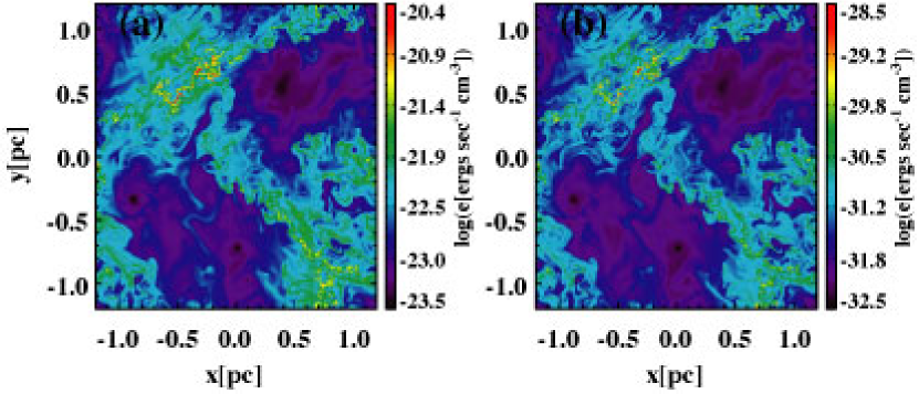
Figure 2: Synthesized (a)[C II] and (b) CO$(1-0)$ line-emissivity distributions in the two-phase flow model at $t=$ 2.479 Myr. Intensities of the emission lines, which are in proportion to the emissivity in the optically thin case, reflect both the density and temperature distributions. Radiation is emitted mainly from tiny, cold, dense clumps.

Since the density is below the critical density for LTE $n_{\mathrm{crit}}(\approx 3000$cm${}^{-3})$ throughout the whole region, and both lines are assumed to be optically thin, line emissivity per unit volume is proportional to $n_{\rm H}^{2}$ under the assumption of uniform abundance distribution. Thus the emissivity map closely resembles the density distribution one. Tiny cold clumps strongly emit radiation in both [C II] and CO$(1-0)$ lines because of high density.

In order to extract outstanding characteristics of two-phase medium, we also perform the simulation of “one-phase” isothermal (10K) turbulent flow with the same resolution ($2048^{2}$ grids). This choice of temperature is based on the conventional assumption in many isothermal turbulence models of dense molecular clouds strongly shielded against UV field (e.g., Padoan et al., 2001). Figure 3 shows the density distributions from a snapshot of the one-phase model. Filamentary structures, which are commonly observed in simulations of isothermal turbulent flow, appear in Figure 3 as well. Sharp edges of filamentary structures imply that they are formed by shock compression.

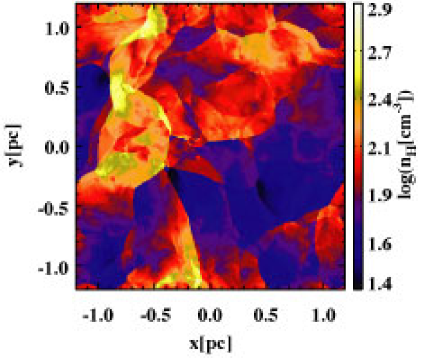
Figure 3: Density distribution in the one-phase flow model at $t=5.248$ Myr. Woven structures with sharp edges are observed, formed through strong shock compression by initial supersonic turbulent motions.

The synthetic emission maps of [C II] 158$\mu$m and CO$(1-0)$ lines, which are calculated in a way similar to those of the two-phase model, are displayed in Figure 4. As in the two-phase model, [C II] and CO$(1-0)$ emission distributions closely trace the density one. For the one-phase model, our emissivity maps agree well with previous work on, for example, synthetic maps of optically thin ¹³CO line of the isothermal model of Padoan et al. (2001).

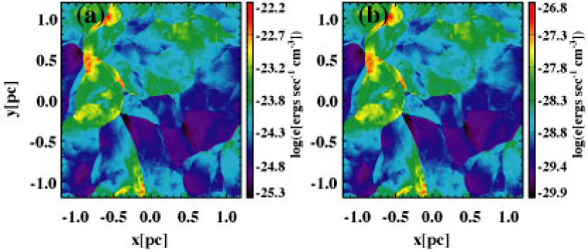
Figure 4: Emissivity distributions of (a) [C II] and (b) CO$(1-0)$ lines in the one-phase flow model with $T=10$K at $t=5.248$ Myr. Highly woven structures are also seen in line-intensity distributions.

3.2 Analyses of Synthetic Line Intensities

To extract characteristic properties of the two-phase models from our calculations, further analysis is required. We simulate realistic observations of a three-dimensional cube by taking one of the axes of our two-dimensional hydrodynamical calculations as a line of sight. Defining the $x$ axis as the line of sight and the $x$ component of the velocity field as the velocity along the line of sight, we can calculate the intensity of the line emission $I(L)$ as

$$I(L)=\frac{1}{4\pi}\sum_{v_{x}}\sum_{x}\frac{d\Lambda_{L}}{dv_{x}}(x,v_{x})\Delta x\Delta v_{x},$$ (7)

where $\Lambda_{L}$ is the emission rate per unit volume on the $L$-th line of sight, $\Delta x$ is the grid size, and $\Delta v_{x}$ is the bin size of the velocity channel, respectively. Straight summation of $\Lambda_{L}$ is applicable because we assume all the lines are optical thin. Hereafter we analyze integrated intensity data obtained by equation (7). Note $\Lambda_{L}$ includes thermal broadening as well as bulk fluid velocity (see eq. 6), and therefore $I(L)$ correctly reflects the velocity structure inherent in the model as well.

3.3 Ratio of High- and Low-Temperature Tracer Lines

A distinguishing feature of the two-phase turbulence model induced by thermal instability is the coexistence of the gases of diversely different thermal conditions. In this section, we investigate characteristics of the two-phase model by simultaneous analysis of two kinds of lines that trace either high- or low- temperature medium. In the following sections, we examine intensity ratios between the [C II] line and CO$(1-0)$ line, CO rotational lines, and C I fine-structure lines.

3.3.1 [C II]-CO(J=1-0) line ratio

Figure 5 displays the $\Lambda_{[{\rm CII}]}-\Lambda_{\rm CO(1-0)}$ ratio (in Figure 5 the ratio of $\Lambda_{[{\rm CII}]}/\Lambda_{\rm CO(1-0)}$ is multiplied by a constant factor $3\times 10^{-7}$ just for clarity of the figure; therefore, in the following arguments, the absolute values of longitudinal axis are in an arbitrary unit, and only the relative positions of the points in the diagram have meaning). The points taken from the one-phase model fall on a straight line of a constant value of $\Lambda_{[{\rm CII}]}/\Lambda_{\rm CO(1-0)}\sim 10^{-2}$, while those from the two-phase model make a slightly bending curve with much larger values of $\Lambda_{[{\rm CII}]}/\Lambda_{\rm CO(1-0)}\gtrsim 10^{2}$ in this diagram.

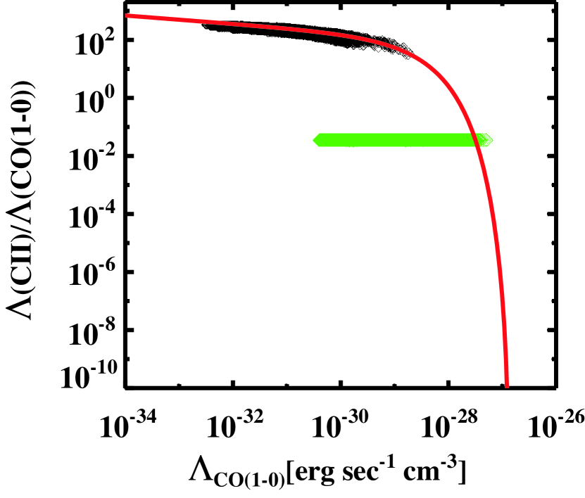
Figure 5: Ratio of emissivities per unit volume, $\Lambda_{\mathrm{[CII]}}/\Lambda_{\mathrm{CO(1-0)}}$ as a function of $\Lambda_{\mathrm{CO}(1-0)}$. The values of $\Lambda_{\mathrm{[CII]}}/\Lambda_{\mathrm{CO(1-0)}}$ are shifted by an arbitrary factor of $3\times 10^{-7}$ for clarity of the figure. The horizontal line located in the lower half consists of dots from the one-phase model, while the upper, slightly bending curve consists of those from the two-phase model. The thin solid curve is the isobaric contour at the saturation pressure $P_{\mathrm{sat}}=10^{3.4}$ K cm^-3.

This difference is interpreted as follows: As we assume that the medium is optically thin, and all the densities in our calculations are below the critical density for both [C II] and CO$(1-0)$ lines ($\approx$ 3000 cm^-3), the line ratio is simply described in terms of $\Lambda$,

$$\frac{I_{\rm[CII]}}{I_{\rm CO(1-0)}}\approx\frac{\Lambda_{\rm[CII]}}{\Lambda_{\rm CO(1-0)}}=\frac{y({\rm C^{+}})\langle\sigma v\rangle_{\rm[CII]}(T)}{y({\rm CO})\langle\sigma v\rangle_{\rm CO(J=1)}(T)}.$$ (8)

In equation (8) $\langle\sigma v\rangle_{\rm[CII]}$ and $\langle\sigma v\rangle_{\rm CO(J=1)}$ are determined by the cross sections for collisional excitations and are dependent only on temperature. In our calculations the abundances of CO and C⁺ are assumed to be uniform, and then equation (8) implies that the ratio $I_{\rm[CII]}/I_{\rm CO(1-0)}$ is a function of temperature. In our one-phase turbulence model of which temperature is adopted to be constant (=10K), the temperature-dependence of equation (8) drops out and the [C II] intensity is linearly proportional to the CO$(1-0)$ intensity (see Figure 5).

On the other hand, the ratio is not constant in the two-phase turbulence model where temperature strongly varies from place to place. In this case, the pressure approaches approximately constant within the whole calculation domain and the points taken from our two-phase model fall on the isobaric contour of $P=P_{\mathrm{sat}}$. We overplot the isobaric contour with $P=P_{\mathrm{sat}}$ with a solid line in Figure 5, which closely trace the dots from our two-phase simulations. Under constant pressure, increasing density indicates decreasing temperature. In the low density (or high temperature $T\gtrsim$ 1000K) limit the cooling rate per unit volume increases with density as $n_{\rm H}^{2}$, and the collisional cross sections $\langle\sigma v\rangle$ are similar for both C⁺ and CO in such a high-temperature regime. Thus $\Lambda_{\mathrm{CO(1-0)}}$ is approximately proportional to $\Lambda_{\mathrm{[CII]}}$. On the other hand, as the temperature decreases below $T\lesssim 100{\rm K}$, $\langle\sigma v\rangle_{\rm[CII]}$ decreases with $T$ much faster than $\langle\sigma v\rangle_{\rm CO(J=1)}$ because of the exponential decrease in the number of particles that can excite the [C II] line (92K). Simultaneous increase in density with a decrease in temperature brings the number of CO molecules in the level $J=1$ close to the LTE limit. Because of the slower decrease in $\langle\sigma v\rangle_{\rm CO(J=1)}$ with temperature compared with $\langle\sigma v\rangle_{\rm[CII]}$, and the saturation of the $J=1$ level population owing to LTE, there is a sharp decline of the isobaric contour toward $\Lambda_{\mathrm{CO(1-0)}}\approx 10^{-27}$ erg sec^-1 cm^-3. This explains the behavior of the isobaric line in Figure 5, which turns downward with increasing density.

3.3.2 CO rotational line ratios

In this subsection, we consider ratios between intensities of CO$(1-0)$ and higher $J$ lines. Since the excitation energies of rotational levels from the ground state $E_{J}/k_{B}=2.75{\rm K}J(J+1)$ increase with $J$, higher $J$ lines trace higher temperature gas. In Figure 6 we show the line intensity ratios $R_{J,(J-1)/10}\equiv I_{\mathrm{CO}(J-(J-1))}/I_{\mathrm{CO}(1-0)}$ for both two-phase and one-phase models. The dependence of line ratios on rotational quantum number $J$ is surprisingly different for these two turbulent flow models.

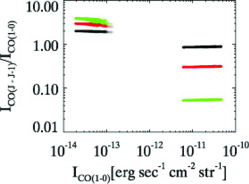
Figure 6: The ratios of intensities of a CO high ($J=2,3,4$) excitation line with the CO$(1-0)$ line. There are two sequences of plots corresponding to the two-phase and the one-phase model, respectively. The green dots are $R_{43/10}$, the red are $R_{32/10}$, and the black are $R_{21/10}$. The left sequence is the two-phase flow data, and the right one is the one-phase flow data. In the two-phase model, the line ratio $R_{J,(J-1)/10}$ increases with $J$, while, in the one-phase model, its dependence on $J$ is opposite for $J\leq$ 4.

In the one-phase model, the line ratios $R_{J,(J-1)/10}$ decrease with increasing $J$, while this trend reverses in the two-phase model up to $J\lesssim 5$: in the one-phase model, although the CO$(2-1)$ line is almost as strong as CO$(1-0)$ line ($R_{21/10}\lesssim 1$), higher $J$ lines become progressively weaker. On the other hand, in the two-phase model, the line ratio $R_{21/10}$ is as large as 2 and $R_{32/10}$ and $R_{43/10}$ become even larger.

This can be explained by the following argument: Since density is lower or at most marginally higher than the critical density ($n_{\rm cr}\sim 3000{\rm cm^{-3}}$) in our snapshots, here we consider the low-density limit. In other words, we discuss the cases where the radiative decay from each level dominates all the collisional transitions both into and from this level, except the collisional excitation from the ground state. Under this assumption, the equations of the detailed balance for the optically thin lines can be approximately described as

$$A_{10}n_{1}=\sum_{J\geq 1}C_{0J}n_{0}$$ (9)

for the ground level ($J=0$) and

$$A_{J+1,J}n_{J+1}+C_{0J}n_{0}=A_{J,J-1}n_{J},$$ (10)

for levels $J\geq 1$. The collisional excitation rate $C_{ij}$ is written as in equation (5). From these equations, we obtain

$$A_{J,J-1}n_{J}=\sum_{J^{\prime}\geq J}C_{0J^{\prime}}n_{0}.$$ (11)

Equation (11) implies that all the CO molecules that are collisionally excited to the state $J$ cascade down to lower levels by spontaneous emission with $\Delta J=1$. Then the downward transition rate from the state $J$ by spontaneous emission is equal to the sum of the collisional excitation rate from the ground state to all the states with $J^{\prime}\geq J$. Using equations (3) and (11), the ratio between the adjacent lines $(J+1)\rightarrow J$ and $J\rightarrow(J-1)$ is

$$R_{(J+1),J/J,(J-1)} = \frac{E_{J+1,J}}{E_{J,J-1}}\frac{\sum_{J^{\prime}\geq J+1}\gamma_{0J^{\prime}}}{\sum_{J^{\prime}\geq J}\gamma_{0J^{\prime}}}$$ (12)

$$= \frac{E_{J+1,J}}{E_{J,J-1}}\frac{G_{J+1}}{1+G_{J+1}},$$ (13)

where $G_{J+1}$ is defined as

$$G_{J+1}=\sum_{J^{\prime}\geq J+1}\frac{\gamma_{J^{\prime}0}}{\gamma_{J0}}\frac{g_{J^{\prime}}}{g_{J}}\exp{\left(-\frac{E_{J^{\prime},J}}{k_{B}T}\right)}.$$ (14)

In the above, we have used the relation

$$\gamma_{0J}=\gamma_{J0}\frac{g_{J}}{g_{0}}\exp{\left(-\frac{E_{J,0}}{k_{B}T}\right)},$$ (15)

where $g_{J}$ is the statistical weight of the level $J$.

Figure 7: Thermal equilibrium curve ($\Gamma=\Lambda$, thick solid curve), and isothermal lines of $T=$ 5000K (dot-dashed), $T=$ 300K (dashed), and $T=$ 50K (dotted : the lowest temperature of the snapshot of two-phase model) in the pressure-density diagram. The saturation pressure $P=P_{\mathrm{sat}}$ is plotted with the thin solid line. The temperature range where bi-stability is possible is limited to 300K$\lesssim T\lesssim$5000K.

In the following, we examine the line intensity ratios using the set of equations (12)-(14) in the low and high temperature limits. In the low temperature limit where $T\ll E_{J+1,J}/k_{B}$, $G_{J+1}$ can be approximated with its first term,

$$R_{(J+1),J/J,(J-1)}\simeq\frac{E_{J+1,J}}{E_{J,J-1}}\frac{\gamma_{J+1,0}}{\gamma_{J,0}}\frac{g_{J+1}}{g_{J}}\exp\left(-\frac{E_{J+1,J}}{k_{B}T}\right).$$ (16)

Equation (16) shows that when the temperature is lower than the excitation energy $E_{J+1,J}/k_{B}$, the line ratio $R_{(J+1),J/J,(J-1)}$ is exponentially reduced. In our one-phase model with $T$=10K, the excitation energy $E_{J,J-1}/k_{B}$ is higher than the kinetic temperature for high $J$ ($J\geq 2$) lines and the line ratio $R_{J,J-1}/R_{10}=\prod_{J^{\prime}=1}^{J}R_{J^{\prime}+1,J^{\prime}/J^{\prime},J^{\prime}-1}$ is significantly smaller than unity. The only exception is $R_{21/10}\sim 1$ since $E_{1,0}/k_{B}=11$K is comparable to the kinetic temperature. On the other hand, in the high-temperature limit where $T\gg E_{J+1,J}/k_{B}$, $G_{J+1}\gg 1$ since numerous terms in the summation of $G_{J+1}$ (eq. [14]) are order of unity. Then,

$$R_{(J+1),J/J,(J-1)}\simeq\frac{E_{J+1,J}}{E_{J,J-1}}.$$ (17)

In our two-phase model, high-temperature regions where high $J$ lines ($T\gtrsim E_{21}/k_{B}$) can be collisionally excited are present. In the snapshot shown in Figure 2, indeed, the temperature ranges from 50K to 3700K which is higher than CO excitation energies up to $J\leq$ 4 ($E_{J}=55$ K) in most of the volume (see Fig. 7). The excitation energies up to $J\leq 4$ are smaller than 50K. Therefore equation (17) is applicable to the whole region and $R_{J,J-1/10}$ becomes order of unity.

3.3.3 [C I] line ratio

In the transition region between the warm atomic region of low density and the cold molecular region of high density, carbon is partly in a neutral atomic form C⁰. In this section, we calculate [C I] fine-structure lines. In the temperature and density range under consideration, important lines are the forbidden transitions among the triplet ${}^{3}P_{2}$, ${}^{3}P_{1}$ and ${}^{3}P_{0}$ in the ground electronic state. In Figure 8, we show the ratio of ${}^{3}P_{1}-^{3}P_{0}$ (24K) and ${}^{3}P_{2}-^{3}P_{1}$ (39K) lines. Similar to CO rotational line ratios, the [C I] line ratio becomes close to unity in the two-phase model, while it is significantly smaller than unity in the one-phase model.

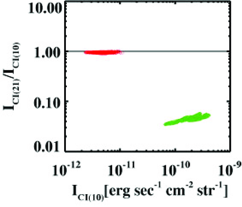
Figure 8: The ratios of C I fine-structure-line intensities $I(^{3}P_{2}-^{3}P_{1})/I(^{3}P_{1}-^{3}P_{0})$ as a function of $I(^{3}P_{1}-^{3}P_{0})$. The two sequences correspond to the one- and two-phase models. The ratios of high- and low-transition-energy lines of C⁰ resemble those of CO molecules: in the two-phase model, the ratio is close to unity, while in the one-phase model the ratio is smaller than 0.1. See discussion in §3.3.2.

This behavior can be understood in a similar way to the argument for CO rotational lines (§3.3.2). Again, we consider the low-density limit. In the following we call levels ${}^{3}P_{0}$, ${}^{3}P_{1}$, and ${}^{3}P_{2}$ levels 0, 1, and 2, respectively. Since the radiative transition from level 2 to 0 is negligible compared with that from level 2 to 1, the equations for statistical balance read

$$A_{21}n_{2}+C_{01}n_{0}=A_{10}n_{1}$$ (18)

for level 1, and

$$C_{02}n_{0}=A_{21}n_{2}$$ (19)

for level 2. From these equations and relations (5) and (15), the line ratio is given by

$$R_{21/10} = \frac{E_{2,1}A_{21}n_{2}}{E_{1,0}A_{10}n_{1}}$$ (20)

$$= \frac{E_{2,1}}{E_{1,0}}\frac{\gamma_{02}}{\gamma_{01}+\gamma_{02}}$$ (21)

$$= 1.625\frac{G}{1+G}$$ (22)

where

$$G = \frac{\gamma_{20}g_{2}}{\gamma_{10}g_{1}}\exp{\left(-\frac{E_{2,1}}{k_{\rm B}T}\right)}$$ (23)

$$= 0.96\left(\frac{T}{100{\rm K}}\right)^{0.12}\exp{\left(-\frac{39{\rm K}}{T}\right)},$$

where we consider only collision with neutral hydrogen as for the excitation partner for numerical evaluation. The above expression clearly expresses that the line ratio becomes close to unity for $T\gtrsim 39{\rm K}$ (as in the two-phase model), while for lower temperature (as in the one-phase model of $T=10$K) it decreases exponentially.

3.3.4 Summary of the Line-ratio Analyses

We have demonstrated in this subsection that the intensity ratio $R_{h/l}$ of lines of high-transition energy ($\Delta E_{h}/k_{B}\approx$ 100K) and low-transition energy ($\Delta E_{l}/k_{B}\approx$ 10K) is as high as unity in the two-phase model, while $R_{h/l}$ is much smaller than unity in the 10K isothermal model. This feature is quite robust and is independent of the species of emitting particles (atomic carbon or CO molecule) and the nature of transitions (fine-structure transitions or rotational transitions). Discussion in §3.3.2 explains the trend in line ratios in terms of the level population in low-density gas. The level populations are determined by collisional excitation and radiative de-excitation by spontaneous emission. In this case the number of particles that have enough energy for level excitation is proportional to $\exp(-\Delta E/k_{B}T)$, and then the level population reflects the ratio of transition energy and kinetic energy, $\Delta E/k_{B}T$. In other words, our results show that simultaneous observation of both high- and low-energy lines from the diffuse atomic/molecular transition region will reveal the thermal structures of the gas. If the high line ratio is observed in such regions in future, we can confirm the existence of two-phase turbulent flows. In the following section, we discuss the implications of our results for the CO line ratio in more detail.

4 Discussion

4.1 Possible CO abundance variation in the warm phase

We have assumed uniform abundance distribution both temporally and spatially for all the species. This assumption appears too artificial if we consider complex chemical reactions in the temperature range $T\lesssim 10^{3}$K. Actual chemical abundances in diffuse clouds will evolve both in space and time, reflecting the environments of the clouds and their evolutionary history, that is, the development of the multi-phase medium. In particular, whether CO is present in such a diffuse environment is quite uncertain. Since line intensity is proportional to the abundance of emitting species in an optically thin medium, the lack of CO in the warm gas would reduce the CO line intensity. In Figure 2a, one can see that warm ($T\sim 1000$K) gas occupies a large fraction of volume in the two-phase medium. In evaluating the CO line intensity by integrating the emissivity along the line of sight (or the $x$ axis in our analysis), we need to take into account the possible deficiency of CO molecules in the warm phase.

To assess the extent of this effect on our results, we perform the following simple experiments: Although formation and destruction rates of CO molecules are dependent on various thermal factors, e.g., density and temperature, the degree of depletion onto dust grains and so on in a complex fashion, it is plausible to assume that the abundance of CO, $y(\mathrm{CO})$ increases with decreasing temperature and increasing density. In our two-phase model, the whole region is approximately in pressure balance. Thus higher density means lower temperature, and CO abundance can be regarded as a function only of temperature, as long as chemical reactions of CO are in equilibrium. As the simplest example, we assume that CO is completely destroyed above a threshold temperature $T_{\mathrm{crit}}$. Namely, the CO abundance $y(\mathrm{CO})$ is taken as a step function of temperature $T$;

$$y(\mathrm{CO})=\cases{3\times 10^{-7}&$T\leq T_{\mathrm{crit}}$,\cr 0&$T>T_{\mathrm{crit}}$.\cr}$$ (24)

We take $T_{\mathrm{crit}}$ as a free parameter and examine the effect of different values $T_{\mathrm{crit}}$ on the line ratios. Figure 7 shows that the medium is thermally unstable in the range of 300K $\lesssim T\lesssim$ 5000K. Therefore the spread of temperature grows as large as this range in our two-phase flow calculations (50K $\lesssim T\lesssim$ 3,700K). We study four cases of $T_{\mathrm{crit}}$ = 100K, 400K, 1000K, and 3000K, which correspond to $n_{H}=40$, 10, 4, and 1.3 cm^-3, respectively, under the saturation pressure $P_{\mathrm{sat}}=10^{3.4}$ K cm^-3. We repeat the same analyses as in §3 for each of $T_{\mathrm{crit}}$.

In Figure 9, we show the CO($J-(J-1)$)/CO$(1-0)$ line ratios for different values of $T_{\mathrm{crit}}$. With a decrease in $T_{\mathrm{crit}}$, the volume occupied by the warm phase (where $y(\mathrm{CO})$ is set to be 0) drastically increases. Radiation is emitted only from surviving cold clumps. In spite of a drastic increase in volume of the warm phase, the line ratios do not change significantly (Figure 9). This result is supported by our discussion in §3.3.2 that the line ratio of CO rotational transitions depends only on the ratio of the excitation energy of the line $\Delta E$, and the kinetic temperature of the gas $k_{B}T$, as long as density is low ($n<n_{\mathrm{crit}}$). As depicted by the isothermal lines in Figure 7, after the system settles onto a constant pressure around the saturation pressure $P_{\mathrm{sat}}$, the lowest temperature of the two-phase model is as high as 50K in our calculation. This lowest temperature assures $E_{J}/k_{B}T<1$ for $J\lesssim 4$ ($T_{J}=$ 55K), so that even in the coldest region in our two-phase model the line ratios $R_{J,(J-1)/10}$ exceed (or are close to) unity. Since CO molecules are preferentially formed in the dense strongly shielded clumps (see also discussion in this section below), the temperature inside the CNM of the two-phase ISM can be lower than our results owing to the resultant CO cooling. In fact, according to Wolfire et al. (1995), the thermal equilibrium temperature in CNM is as low as $\sim$ 20K. The condition for high line ratio $E_{J}/k_{B}T<1$ becomes more difficult to be satisfied in colder CNM: the line ratio is accordingly lowered. Thus, the value of $R_{J,(J-1)/10}$ of higher $J$ is reduced, while $R_{21/10}$ stays the same as our results except in strongly shielded molecular clouds of 10K owing to the very low excitation energy only 16.5K. In this case we should use the line ratio $R_{J,(J-1)/10}$ of low $J$ lines to study the thermal structure of the CNM.

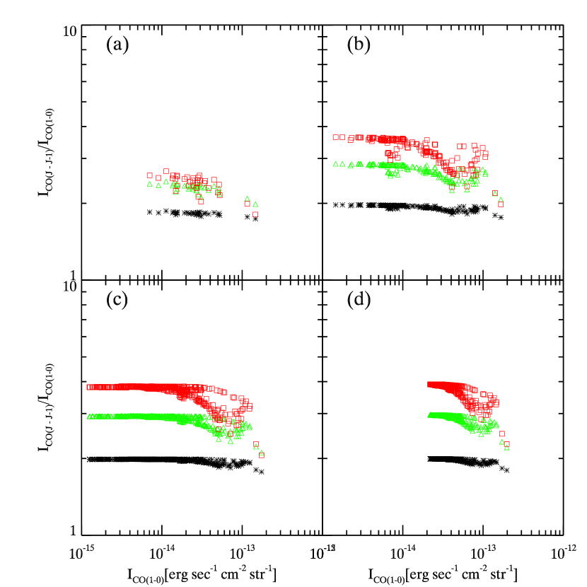
Figure 9: CO rotational line ratios with different values of threshold temperature $T_{\mathrm{crit}}$, above which CO abundance is set to zero. Dots of each color correspond to the same transition $J$ as those displayed in Figure 6. The threshold temperatures are (a) $T_{\mathrm{crit}}=100$K, (b) 400K, (c) 1000K, and (d) 3000K. If the pressure is at the saturation value $P_{\mathrm{sat}}=10^{3.4}$ K cm^-3, the equivalent threshold densities are (a) 40 cm^-3, (b) 10 cm^-3, (c)4 cm^-3, and (d) 1.4cm^-3, respectively. One can observe that as $T_{\mathrm{crit}}$ increases, the value of $I(\mathrm{CO(1-0)})$ increases. This is because emission from the warm gas is added to the summation along the line of sight. Also the values of the ratio do not change significantly, because, even in the coldest regions, the energy difference of the levels $\Delta E/k_{B}T<1$ in the two-phase model (see discussion in §3.3.2).

The increase in the threshold temperature $T_{\mathrm{crit}}$ is accompanied by an increase in the average temperature $T$ in the emission region. Since the line ratio $R_{J,(J-1)/10}$ grows larger as the average temperature $T$ increases (§3.3.2), the shift of the threshold temperature $T_{\mathrm{crit}}$ does not alter the trend toward the averaged $R_{J,(J-1)/10}>1$ as long as $\Delta E/k_{B}T<1$. Note that our simple experiments include two extreme cases of high- and low- $y(\mathrm{CO})$ values in the warm phase. Thus we conclude that, as long as we are concerned with the line-ratio analysis presented in this article, the result is not significantly affected by complicated chemical evolution. In other words, the line ratio, not the intensity of each line, is a good observational tool for understanding the thermal structure of turbulent interstellar medium.

Since the chain reaction for formation of CO molecules starts with a reaction involving H₂, the presence of H₂ is a necessary condition for CO formation. H₂ molecules are formed via association of two hydrogen atoms on the surface of dust grains. The formation timescale of H₂ molecules is described as $\tau_{\mathrm{H}_{2}}=1.67\times 10^{9}n_{\rm H}^{-1}$ years (Spitzer 1978). The formation timescale becomes on the order of $10^{6}$ years in the dense cold clumps, where $n_{H}\gtrsim 10^{3}$ cm^-3. Then if the dense clumps survive as long as $10^{6}$ years, CO molecules can form inside. There are some arguments supporting the existence of CO molecules in tenuous warm ISM. Recently, Inoue, Inutsuka & Koyama (2006) emphasized the importance of gas flows (i.e. evaporation) from cold phase to warm phase. If molecules are abundant inside the cold clouds, they will be dispersed into the warm phase. The efficient evaporation of CO from cold clumps enables the supply of CO molecules to the warm gas on a relatively short timescale, although the chemical timescale is much longer than other relevant timescales in the warm phase. Of course, if the UV radiation is as intense as in average diffuse ISM, such CO molecules would be photodissociated immediately. Hennebelle & Inutsuka (2006) proposed an alternative model for cold molecular clouds that possess warm gas deep inside. In this picture, CO molecules can avoid photodissociation within such warm neutral medium (WNM) because external UV radiation is blocked by the surrounding cold molecular gas. In this scenario, the condition $\Delta E/k_{B}T<1$ is satisfied for CO molecules in WNM.

Here we discuss two possible evolutionary scenarios for CO abundance in diffuse ISM. First, we consider the case of relatively strong interstellar UV radiation, stronger than the adopted value ($G_{0}=1$ in our article). If there were a large number of FUV photons, CO molecules would be easily photodissociated. The shielding of UV photons by atomic and molecular hydrogen and dust grains would result in selective destruction of CO molecules in the tenuous warm medium, but CO molecules in dense, cold clumps, surrounded by a warm medium, would be protected against UV penetration. Another possibility is that a strong UV field might thermally stabilize the medium at a single warm phase (Wolfire et al., 1995). In this case, however, CO molecules would not be able to survive photodissociation and CO line emission would be very weak, even though there are some turbulent flows. The survey observations of molecular clouds in the Galactic plane suggest that the number of regions of high-line ratio $R_{21/10}\gtrsim 1.0$ is small (Sakamoto et al., 1997; Oka et al., 1998). These results might be interpreted as a signature of the lack of initial CO molecules by photodissociation. If this is the case, more refractory molecules must be used as tracers of the two-phase medium. In order to examine what transitions can be better tracers, it is necessary to include greater detail of chemical evolution in our hydrodynamical simulations, as well as of the evolution of the main cooling and heating sources. Second, we consider the case of weak UV irradiation as we have considered in this article. In our two-phase models, the temperatures do not exceed $T\approx$ 5000K, and CO molecules once formed are not subject to the collisional dissociation. In this case, our experiments in this subsection are straightforwardly applicable and the ratio of rotational transitions of CO molecules is a good probe of thermal structure in the turbulent ISM.

4.2 Comparison with Observational Results

4.2.1 Related Observations of Diffuse Clouds

The effective cooling function we adopted (equation 2) was calculated under the condition of small visual extinction, $A_{V}\lesssim 0.1$. This environment corresponds to the periphery of molecular clouds where the composition of carbon changes from atomic to molecular form. Sakamoto & Sunada (2003) found peculiar structures in the position-velocity (P-V) diagram around $A_{V}\lesssim 1$ in their observations of CO$(1-0)$ in Taurus HCL2, which spans over a wide range of $A_{V}$. Tiny clumps with sharp velocity gradients of radius $R\approx 0.05$pc suddenly appeared when $A_{V}$ fell below unity in all of three observed strips. They speculated that these structures were cold dense clumps formed by thermal instability since this instability under mild UV heating occurred approximately around $A_{V}\sim 1$. In Figure 10 we display the synthetic P-V diagram of CO$(1-0)$ line from the snapshots of the simulations at 3 Myr. The two-phase model shows that velocity of clumpy structures spreads over a wide range ($\Delta v_{r}\approx$ 5 km sec^-1). Indeed, our synthetic P-V diagram of the two-phase model looks quite similar to that of Sakamoto & Sunada (2003) at $A_{V}\lesssim$1. Since our simulations do not consistently include the spatial variation of UV shielding in modeling periphery of molecular clouds, direct comparison with these observational results should be done with caution. This similarity is, however, quite encouraging for confirming our two-phase model driven by UV photoelectric heating.

IRAM observations of starless molecular clouds also suggest the possibility that tiny gas clumps are filling the beam (Falgarone et al., 1998). Furthermore, in more diffuse regions in the Galactic plane, ISO observations of H₂ rotational lines suggest the existence of collisionally heated warm gas ($T\lesssim 10^{3}$K) within the cold diffuse ISM (Falgarone et al., 2005). Although both of the observed regions are denser than our calculations, their structures might be roughly consistent with the two-phase medium models generated by UV photoelectric heating (Koyama & Inutsuka, 2002; Audit & Hennebelle, 2005) or dissipative heating of Alfvén waves (Hennebelle & Inutsuka, 2006). We can clarify the nature of the multi-phase ISM by making comparisons with line-emission calculations like ours and such detailed observations of diffuse ISM as described above.

4.2.2 Comments on observations of the CO line ratio $R_{21/10}$

Despite our conclusion that the two-phase medium has a high line-ratio $R_{J,J-1/10}=$

$I_{\mathrm{CO}(J-(J-1))}/I_{\mathrm{CO}(1-0)}\gtrsim$ 1.0, observations have found that regions of high line-ratio $R_{21/10}=$ $I_{\mathrm{CO}(2-1)}/I_{\mathrm{CO}(1-0)}$ $\gtrsim$ 1.0 are of limited fraction (Sakamoto et al., 1997; Oka et al., 1998) and usually only appear close to HII regions. Our results of high $R_{21/10}$ values are in part due to the assumption of small optical thickness ($\tau\ll$ 1). If we included the effect of finite optical thickness, the line ratio $R_{21/10}$ averaged over the simulation box would become smaller. However, as for the peripheral regions, which are optically thin, our treatment is still valid and our conclusions should not be altered. Discrepancy between existing observations and our prediction is probably due to the fact that observations tend to be strongly biased to clouds with high CO intensity, thus having higher average density compared with the transition regions we discussed. To observationally examine the atomic/molecular transition regions, we must take care not to include both high and low CO intensity regions in a single observing beam in resolving the spatial gradient of $A_{V}$. For this purpose, observations not only with high angular resolution but also with high sensitivity are needed for achieving high S/N observation of faint transition regions, avoiding contamination of high intensity regions. We hope that future instruments will provide a good information for the two-phase scenario of ISM turbulence.

Here we discusss some of the characteristics of the cold clumps analyzed in this paper and future observation. The typical size of the cold clumps is determined by the maximum growth wavelength in thermally unstable medium $\lambda_{\mathrm{MGR}}\approx\sqrt{\lambda_{\mathrm{F}}\lambda_{\mathrm{cool}}}$ (Field, 1965), where $\lambda_{\mathrm{F}}=(KT/{n_{\rm H}}^{2}\Lambda)^{1/2}$ is the Field length, and $\lambda_{\mathrm{cool}}=c_{s}\cdot(3/2)k_{\rm B}T/({n_{\rm H}}\Lambda)=c_{s}\tau_{\mathrm{cool}}$ is the cooling length, respectively. Numerically these values are

$$\lambda_{\mathrm{F}} = 7.6\times 10\left(\frac{T}{\mathrm{300K}}\right)^{3/2}\left(\frac{n_{\rm H}\Lambda}{10^{-25}{\rm erg~{}sec^{-1}}}\right)^{-1/2}$$ (25a)

$$\left(\frac{n_{\rm H}}{\mathrm{100cm}^{-3}}\right)^{-1/2}\mathrm{AU,}$$

$$\lambda_{\mathrm{cool}} = 3.6\times 10^{3}\left(\frac{T}{\mathrm{300K}}\right)^{3/2}\left(\frac{n_{\rm H}\Lambda}{10^{-25}{\rm erg~{}sec^{-1}}}\right)^{-1}\mathrm{AU,}$$

$$\lambda_{\mathrm{MGR}} = 5.3\times 10^{2}\left(\frac{T}{\mathrm{300K}}\right)^{3/2}\left(\frac{n_{\rm H}\Lambda}{10^{-25}{\rm erg~{}sec^{-1}}}\right)^{-3/4}$$ (25c)

$$\left(\frac{n_{\rm H}}{\mathrm{100cm}^{-3}}\right)^{-1/4}\mathrm{AU,}$$

where ${n_{\rm H}\Lambda}$ is cooling rate per particle, and the normalizations are taken from typical values in our calculation. If tiny cold clumps reside at the distance of nearby molecular clouds $D=$ 140pc, the angular size of a clump of radius $\lambda_{\mathrm{MGR}}=5.3\times 10^{2}$AU is $\sim 3.7^{\prime\prime}$. From Figures 6, 8 and equation (7) intensities of CO($1-0$) and [C I] lines of the two-phase medium are $I(\mathrm{min})\gtrsim 10^{-13}(\Delta x/2.4\mathrm{pc})$ erg sec^-1 cm^-2 str^-1 in our calculations (where $\Delta x$ is the total length scale of the two-phase medium along the line of sight). This intensity value corresponds to the brightness temperature $T_{b}=2.46\times 10^{-4}$K ($\Delta x/2.4\mathrm{pc}$)K, and is too weak to be detected with ALMA telescope unless the line-of-sight length of the cloud is sufficiently large (ALMA Sensitivity Calculator), even though its high angular resolution is sufficient for resolving each tiny clump. This might suggest that we should target near-by clouds such as some of the high latitude clouds (e.g., Magnani, Blitz & Mundy, 1985). In addition to the weak average intensity, the volume filling factor of the tiny CNM clumps of which intensity dominates, is much less than unity (Fig. 2). Taking into account of these difficulties, we should be careful in the interpretation of the observations for the tiny CNM clumps in the diffuse two-phase ISM even with ALMA.

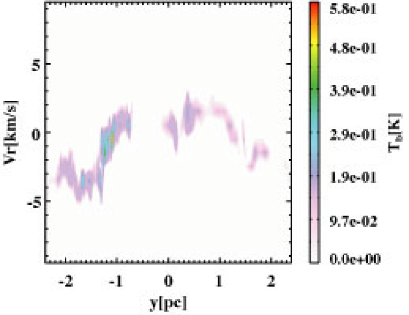
Figure 10: Synthetic position-velocity diagram of the CO$(1-0)$ line at $\sim$ 3Myr snapshots of the two-phase model. Tiny structures spread with a velocity dispersion of $\Delta v_{r}\sim 5$ km/s.

On the other hand, Figure 10 shows that the tiny clump-like structures are assembled into larger structures of $\lesssim$ 0.1 pc when integrated along a line of sight in the P-V diagram. The flux density of such assembly is

$$F_{\nu} = 0.38\left(\frac{I}{1\times 10^{-13}\mathrm{erg}~{}\mathrm{sec}^{-1}~{}\mathrm{cm}^{-2}~{}\mathrm{str}^{-1}}\right)\left(\frac{\Delta v_{x}}{1\mathrm{km}~{}\mathrm{sec}^{-1}}\right)^{-1}\left(\frac{\Delta x}{2.4\mathrm{pc}}\right)$$ (26)

$$\times\left(\frac{R}{0.05\mathrm{pc}}\right)^{2}\left(\frac{D}{140\mathrm{pc}}\right)^{-2}~{}~{}\mathrm{mJy},$$

which might be observable with a future telescope equipped with highly sensitive receivers. For better evaluation of the intensity, we need to study the global structure of the atomic/molecular transition region which supposedly consists of the tiny clump-like structures appeared in our simulations. Such a global modelling is beyond the scope of this paper, but should be included in future simulations.

When future highly sensitive multi-$J$ line observations of “peculiar” structures with typical size $\sim$ 0.1pc detected in the strip-scanned CO($1-0$) data (Sakamoto & Sunada 2003; see §4.2.1) are available, they will greatly improve our understandings of their origin and identity. In those rims of molecular clouds with $A_{V}\lesssim 1$, even smaller structures might be found with future deep observations. Small ($\lesssim$ 0.1 pc) structures with high-line ratio in imaging observations would be the best verification of the two-phase ISM turbulence models and of the formation scenarios of molecular clouds based on the multi-phase turbulence models (e.g., Koyama & Inutsuka, 2000; Bergin et al., 2004). Detailed observations using forthcoming powerful instruments will reveal the thermal structure in diffuse interstellar medium, as well as in dense molecular clouds. We hope our calculation of the carbon line ratio would be a prototype to study the nature of ISM using forthcoming high quality observational data.

5 Summary and Conclusion

We examined observational characteristics of the two-phase turbulence model by combining hydrodynamical simulations and radiation calculations. We modeled the diffuse interstellar medium irradiated by UV radiation of $G_{0}=1$, attenuated with an average visual extinction of $A_{V}\sim 0.1$. In our model settings, the two-phase structures are formed by photoelectric heating, and therefore our model corresponds to the atomic/molecular transition region at the periphery of dense molecular clouds. In order to examine such transition regions, we calculated line intensities based on nonLTE level populations for three species of carbon, C⁺, C⁰, and CO. By comparing two line intensities of high- and low- temperature tracers, we found that the line ratio $R_{h/l}$ distinctly reflects the thermal structure of the medium. The results of our analyses showed that, in the two-phase model, higher transition energy lines can be stronger than those of lower energy as long as $\Delta E/k_{B}T<1$. Our argument on the level population in low-density limit ($n<n_{\mathrm{crit}}$) demonstrated that the line ratio of high- and low- temperature tracers are determined by the ratio of transition energy and gas kinetic energy, $\Delta E/k_{B}T$. In addition to uniform abundance calculations, we also analyzed cases where CO is dissociated above a threshold temperature, or equivalently, below a threshold density. Our analyses showed that abundance distribution of CO molecules in the warm phase does not significantly affect the high line ratio that characterize the two-phase model, as long as CO molecules are not completely photodissociated. This is because, even in the coldest regions in our two-phase model, the temperature is as high as 50K ($\approx E_{4}/k_{B}$, the energy level of $J=4$ of the CO rotational transition), and satisfies $\Delta E/k_{B}T<1$. By seeking these features in the diffuse atomic/molecular transition regions, we will be able to confirm the existence of two-phase interstellar turbulence by using the high angular resolution and high sensitivity of future instruments.

References

- Audit & Hennebelle (2005) Audit, E., & Hennebelle, P. 2005, A&A, 433, 1.
- Bergin et al. (2004) Bergin, E. A., Hartmann, L. W., Raymond, J. C. & Ballesteros-Paredes, J. 2004, ApJ, 621, 921.
- de Jong et al. (1980) de Jong, Dalgarno, & Boland, 1980, A&A, 91, 68.
- Elmegreen & Scalo (2004) Elmegreen, B. G., & Scalo, J. 2004, ARA&A, 42, 211.
- Falgarone et al. (1998) Falgarone, E., Panis, J.F., Heithausen, A., Pérault, M. , Stutzki, J., Puget, J.L., & Bensch, F. 1998, A&A, 331, 669
- Falgarone et al. (2005) Falgarone, E., Verstraete, L., Pineau des Forêts, G. & Hily-Blant, P. 2005, A&A, 433, 997.
- Field (1965) Field, G. 1965, ApJ, 142, 531.
- Hattori et al. (1969) Hattori, T., Nakano, T. & Hayashi, C. 1969, Prog. Theor. Phys. 42. 781.
- Heitsch et al. (2005) Heitsch, F., Burkert, A., Hartmann, L.W., Slyz, A. D., & Devriendt, J. E. G. 2005, ApJ 633, L113
- Hennebelle & Pérault (1999) Hennebelle, P. & Pérault, M. 1999, A&A 351, 309.
- Hennebelle & Pérault (2000) Hennebelle, P. & Pérault, M. 2000, A&A 359, 1124.
- Hennebelle & Inutsuka (2006) Hennebelle, P. & Inutsuka, S. 2006, ApJ, 647, 404.
- Hollenbach & McKee (1989) Hollenbach, D. & McKee, C. F. 1989, ApJ, 342, 306.
- Inoue, Inutsuka & Koyama (2006) Inoue, T., Inutsuka, S., & Koyama, H. 2006, ApJaccepted (astro-ph/0604564).
- Inutsuka, Koyama & Inoue (2005) Inutsuka, S., Koyama, H., & Inoue, T. 2005, AIPC. proc. 784, 318.
- Koyama & Inutsuka (2000) Koyama, H., & Inutsuka, S. 2000, ApJ, 532, 980.
- Koyama & Inutsuka (2002) Koyama, H., & Inutsuka, S. 2002, ApJ, 564, L97.
- Koyama & Inutsuka (2004) Koyama, H., & Inutsuka, S. 2004, ApJ, 602, L25.
- Koyama & Inutsuka (2006) Koyama, H., & Inutsuka, S. 2006, submitted to ApJ, astro-ph/0605528.
- Kritsuk & Norman (2002a) Kritsuk, A. G., & Norman, M. L. 2002, ApJ, 580, L51.
- Kritsuk & Norman (2002b) Kritsuk, A. G., & Norman, M. L. 2002, ApJ, 596, L127.
- Larson (1981) Larson, R. B. 1981, MNRAS, 194, 809.
- Mac Low & Klessen (2004) Mac Low, M.-M. & Klessen, R. S. 2004, Rev. Modern. Phys. 76, 125
- Magnani, Blitz & Mundy (1985) Magnani, L., Blitz, L., & Mundy, L. 1985, ApJ, 295, 402.
- McKee & Ostriker (1977) McKee, C. F., & Ostriker, J. P. 1977, ApJ, 218, 148.
- McKee et al. (1982) McKee, C. F., Storey, J. W. V., Watson, D. M., & Green, S. 1982, ApJ, 259, 647-656.
- Nakano (1998) Nakano, T. 1998, ApJ, 494, 587
- Oka et al. (1998) Oka, T., Hasegawa, T., Handa, T., Hayashi, M., & Sakamoto, S. 1996, ApJ, 460, 334
- Padoan et al. (2001) Padoan, P., Juvela, M. Godman, A. A., & Nordlund, A. 2001, ApJ, 553, 227.
- Parker (1953) Parker, E. N. 1953, ApJ, 117, 431.
- Pavlovski et al. (2002) Pavlovski, G., Smith, M. D., Mac Low, M., & Alexander, R. 2002, MNRAS, 337, 477.
- Pavlovski et al. (2005) Pavlovski, G., Smith, M. D., & Mac Low, M. 2005, astro-ph/0504504
- Sakamoto et al. (1997) Sakamoto, S, Hasegawa T., Handa T., Hayashi, M., & Oka, T. 1997, ApJ, 486, 276.
- Sakamoto & Sunada (2003) Sakamoto, S., & Sunada, K. 2003, ApJ, 594, 340.
- Spitzer (1978) Spitzer, L. Jr., 1978, ”Physical Processes in the Interstellar Medium”, Wiley & Sons, Inc.
- Stahler & Palla (2004) Stahler, S. W., & Palla, F. 2004, “The Formation of Stars”, WileyVCH.
- Vazquez-Semadeni et al. (2006) Vazquez-Semadeni, E., Ryu, D., Passot, T., Gonzalez, R. F., & Gazol, A. 2006, ApJ643, 245.
- Wolfire et al. (1995) Wolfire, M. G., Hollenbach, D., McKee, C.F., Tielens, A. G. G. M., & Bakers, E. L. O. 1995, ApJ, 443, 152.