Iron line and diffuse hard X-ray emission from the starburst galaxy M82

Abstract

We examine the properties of the diffuse hard X-ray emission in the classic starburst galaxy M82. We use new Chandra ACIS-S observations in combination with reprocessed archival Chandra ACIS-I and XMM-Newton observations. We find $E\sim 6.7$ keV Fe He$\alpha$ emission (from highly ionized iron) is present in the central $|r|<200$ pc, $|z|<100$ pc of M82 in all datasets at high statistical significance, in addition to a possibly non-thermal X-ray continuum and marginally significant $E=6.4$ keV Fe $K\alpha$ line emission (from weakly ionized iron). No statistically significant Fe emission is found in the summed X-ray spectra of the point-like X-ray sources or the ULX in the two epochs of Chandra observation. The total nuclear region iron line fluxes in the 2004 April 21 XMM-Newton observation are consistent with those of the Chandra-derived diffuse component, but in the 2001 May 6 XMM-Newton observation they are significantly higher and also both E=6.4 and E=6.9 keV iron lines are detected. We attribute the excess iron line emission to the Ultra-Luminous X-ray source in its high state. In general the iron K-shell luminosity of M82 is dominated by the diffuse component. The total X-ray luminosity of the diffuse hard X-ray emission (corrected for emission by unresolved low luminosity compact objects) is $L_{\rm X,2-8keV}\sim 4.4\times 10^{39}\hbox{${\rm\thinspace erg}{\rm\thinspace s}^{-1}\,$}$ in the $E=2$ – 8 keV energy band, and the 6.7 keV iron line luminosity is $L_{\rm X,6.7keV}\sim$(1.1 – 1.7) $\times 10^{38}\hbox{${\rm\thinspace erg}{\rm\thinspace s}^{-1}\,$}$. The diffuse hard X-ray continuum is best fit with power law models of photon index $\Gamma\sim 2.5$ – 3.0, although thermal bremsstrahlung model with $kT\sim 3$ – 4 keV are also acceptable. A simple interpretation of the hard diffuse continuum is that it is the bremsstrahlung associated with the 6.7 keV iron line emission. This interpretation is problematic as it would imply an unrealistically low gas-phase iron abundance $Z_{\rm Fe}\sim 0.4Z_{\rm Fe,\odot}$, much lower than the super-Solar abundance expected for supernova ejecta. We explore the possibility of non-equilibrium ionization, but find that this can not reconcile the continuum and iron line emission. Nor can Inverse Compton X-ray emission be the dominant source of the diffuse continuum as theory predicts flatter power law slopes and an order of magnitude less continuum flux than is observed. The 6.7 keV iron line luminosity is consistent with that expected from the previously unobserved metal-enriched merged supernova ejecta that is thought to drive the larger-scale galactic superwind. The iron line luminosity implies a thermal pressure within the starburst region of $P/k\sim 2\times 10^{7}{\rm K}\hbox{${\rm\thinspace cm}^{-3}\,$}$ which is consistent with independent observational estimates of the starburst region pressure.

1. Introduction

Starburst galaxies – objects with intense recent star formation – have galaxy-sized outflows with velocities in excess of several hundred to a thousand kilometers per second. These superwinds are common in the local Universe, occurring in nearly all galaxies classified as undergoing starburst activity (Lehnert & Heckman, 1995; Heckman, 1998), and appear ubiquitous among the Lyman break galaxies at redshift $\sim 3$ where they are blowing $\sim 100$ kpc sized holes in the IGM (e.g.  Pettini et al., 2001; Adelberger et al., 2003).

Superwinds are believed to be driven by the thermal and ram pressure of an initially very hot ($T\sim 10^{8}$ K), high pressure ($P/k~{}\sim 10^{7}{\rm K}\hbox{${\rm\thinspace cm}^{-3}\,$}$) and low density wind, itself created from the merged remnants of very large numbers of core-collapse supernovae (SNe), and to a lesser extent the stellar winds from the massive stars, that occur over the $\sim 100$ Myr duration of a typical starburst event (Chevalier & Clegg, 1985). Direct observational detection of gas this hot through X-ray spectroscopy or imaging has only recently become possible because of the high spatial resolution of Chandra X-ray Observatory, as starburst regions are also home to large numbers of X-ray-luminous accreting neutron stars and black holes that must be resolved out in order to see any diffuse hard X-ray emission.

All known superwinds were detected through observations of ambient disk or halo gas that has been swept-up by the hotter but more tenuous wind of merged SN ejecta, which has itself escaped direct observational detection until recently. The majority of nearby superwinds have been discovered using optical imaging and spectroscopy to identify outflow in the warm ionized medium (WIM, $T\sim 10^{4}$ K), in many cases directly imaging bipolar structures aligned with the host galaxy minor axis that have kinematics indicative of outflow at velocities of $v_{\rm WIM}=$ a few $\times 100$ to $1000\hbox{${\rm\thinspace km}{\rm\thinspace s}^{-1}\,$}$ (e.g.  Axon & Taylor, 1978; Heckman, Armus, & Miley, 1987; Bland & Tully, 1988; Heckman, Armus, & Miley, 1990; Lehnert & Heckman, 1995, 1996). McCarthy et al. (1987), Heckman et al. (1990), and Lehnert & Heckman (1996) use this entrained low-filling factor gas as a tracer of the pressure in the inner kiloparsec or so of many nearest brightest superwinds, and find the very high central pressures and radial variation in pressure expected from the Chevalier & Clegg (1985) wind model for the thermalized SN ejecta within the vicinity of the starburst region. Superwinds from galaxies at high redshift are recognized by virtue of blue-shifted interstellar absorption lines from warm-neutral and warm-ionized gas species (Pettini et al., 2000; Frye et al., 2002), absorption features very similar to those seen in local starburst galaxies with superwinds (Phillips, 1993; Kunth et al., 1998; González Delgado et al., 1998; Heckman et al., 2000). Nearby superwinds have also been extensively studied in soft X-ray emission (e.g.  Dahlem et al., 1998; Strickland et al., 2004) which probes emission from hot gas with temperatures in the range $T\sim 10^{6}$ to $10^{7}{\rm K}$, following their initial detection by Einstein X-ray observatory (Watson, Stanger, & Griffiths, 1984; Fabbiano & Trinchieri, 1984). Indeed, observations have demonstrated that all phases of the ISM found in normal late type galaxies are also incorporated into starburst-driven superwinds (see the review of Dahlem, 1997).

However, prior to the launch of the Chandra X-ray Observatory (CXO) in 1999, there had been no believable detection of thermal X-ray emission from the $T\sim$ a few $\times 10^{7}$ to $10^{8}$ K merged SN ejecta whose thermal pressure initially drives the superwind in any starburst galaxy. This very hot plasma should be a source of thermal bremsstrahlung in the hard X-ray energy band, as well as strong $E\approx 6.7$ and (possibly) $6.9$ keV emission from highly-ionized Helium-like and Hydrogen-like iron. Hard X-ray emission had been previously been detected from nearby starburst galaxies such as M82 and NGC 253 with X-ray observatories such as EXOSAT (Schaaf et al., 1989), Ginga (Tsuru et al., 1990), ASCA (Ptak et al., 1997; Tsuru et al., 1997) and BeppoSAX (Persic et al., 1998; Cappi et al., 1999). However, the poor-to-nonexistent spatial resolution of these observations prevented a clean assessment of the relative contribution to the hard X-ray emission from compact accreting objects and from any truly diffuse component (the half power enclosed angular diameter of the point spread function (PSF) of BeppoSAX and ASCA at $E\sim 6{\rm\thinspace keV}$ were $r_{50}\sim 2\arcmin$ and $\sim 3\arcmin$ respectively. This was the highest spatial resolution available for any hard X-ray observatory before the launch of Chandra. Assuming a distance of 2.6 Mpc to NGC 253 and 3.6 Mpc to M82, an angular size of $2\arcmin$ corresponds to a physical size of $1.5{\rm\thinspace kpc}$ for NGC 253 and $2.1{\rm\thinspace kpc}$ for M82).

Nevertheless it was clear that the majority of the hard X-ray emission from these galaxies came from compact objects. The observed total hard X-ray luminosities of these galaxies were $\gtrsim 1.5$ orders of magnitude higher than expected from the the very hot gas in a superwind model (Strickland & Stevens, 2000). Both the ASCA and BeppoSAX observations of M82 and NGC 253 also discovered emission possibly due to high ionized iron (Ptak et al., 1997; Tsuru et al., 1997; Persic et al., 1998; Cappi et al., 1999), although this emission was of low equivalent width. The weakness of the Fe K-shell emission implied sub-Solar Fe abundances ($Z_{Fe}\lesssim 0.3Z_{Fe,\odot}$), a peculiar result given that super-Solar abundances ($Z_{Fe}\sim 5Z_{Fe,\odot}$) are expected from pure core-collapse SN ejecta. Alternatively the hard X-ray emission could be dominated by non-thermal continuum emission, possibly from X-ray binaries, thus reducing the equivalent width of the Fe line from the diffuse hot gas. Furthermore, some Galactic X-ray binaries do show Fe K-shell emission (e.g. see Vrtilek, Soker, & Raymond, 1993), so the Fe emission observed in M82 and NGC 253 might come from compact objects rather than any diffuse gas. Despite the low spatial resolution of ASCA, the hard X-ray emission in NGC 253 was distributed so broadly over the disk of the galaxy that Ptak et al. (1997) were able to resolve multiple individual hard X-ray sources. These were also directly associated with point-like X-ray sources seen in soft X-ray observations with the ROSAT High Resolution Imager (HRI). The strong temporal variability in the hard X-ray luminosity of M82 (Ptak & Griffiths, 1999; Matsumoto & Tsuru, 1999) demonstrated that one or more accreting compact objects dominated the hard X-ray emission at some, and possibly all, epochs.

The on-axis half-enclosed-power PSF diameter of Advanced CCD Imaging Spectrometer (ACIS) on the Chandra X-ray Observatory is $0\farcs 8$, a factor of $150$ smaller than BeppoSAX, and also considerably better than the equivalent value of $\sim 13$ – $15\arcsec$ for the MOS and PN detectors on XMM-Newton. The angular diameter of the starburst region in M82 is $\sim 45\arcsec$ (see e.g.  Golla, Allen, & Kronberg, 1996), while that of NGC 253 is $\lesssim 15\arcsec$ (Ulvestad & Antonucci, 1997; Forbes et al., 2000). It is clear that Chandra is the first, and only, X-ray instrument with spatial resolution high enough to resolve the starburst regions in even the nearest starburst galaxies such as M82 and NGC 253.

Using the spectral-imaging CCDs of the ACIS-I camera of Chandra, (Griffiths et al., 2000) detected diffuse hard X-ray emission coincident with the nuclear starburst region of M82. They interpreted the spectrum of this diffuse emission at thermal bremsstrahlung from a hot plasma of temperature $T\sim 4\times 10^{7}{\rm K}$. This was motivated by the detection of excess emission in the energy range $E=5.9$ to 6.9 keV which they attributed to unresolved line emission from highly-ionized iron. This feature that would not be expected if the diffuse X-ray emission where non-thermal in origin, for example inverse Compton (IC) scattering of IR photons off relativistic electrons. This work was based on ACIS-I observations taken in late 1999, soon after the cosmic-ray-induced damage to front-illuminated ACIS-I CCDs had been discovered. As a result, the spectral calibration of these observations was especially difficult. In particular, the radiation-induced reduction in spectral resolution and absolute energy scale calibration of the instrument made it difficult to be sure that Fe emission feature was indeed real.

ACIS-S observations also uncovered diffuse hard X-ray emission in the compact nuclear starburst region of NGC 253 (Weaver et al., 2002). The emission is strongest within the central $5\arcsec$ of the galaxy, and showed a strong hard X-ray emission line spectrum with features attributable to Si, S, Ca and Fe (the back-illuminated chips on ACIS-S suffered less radiation damage than the front-illuminated chips, and hence have higher spectral resolution). This spectrum is more reminiscent of a highly photoionized plasma than a collisionally ionized plasma. As there is independent evidence for a low luminosity AGN (LLAGN) in the center of NGC 253 (Ulvestad & Antonucci, 1997), Weaver et al. (2002) suggest that the diffuse hard X-ray emission from NGC 253 is dominated by gas photoionized by the LLAGN.

Thus the nature of this diffuse hard X-ray emission in M82, and its possible relationship to the very hot merged SN ejecta thought to drive M82’s superwind, has not yet been resolved and is the focus of this paper. We emphasize that M82 is the best case for exploring the properties of diffuse very hot gas created by starburst activity, as the diffuse hard X-ray emission is brighter and has a larger angular extent than in NGC 253. Furthermore, there is no known LLAGN in M82 to complicate matters.

In this paper we make use of the longest available Chandra ACIS and XMM-Newton observations and the most recent instrumental calibrations to further investigate the properties of the diffuse hard X-ray emission in this archetypal starburst galaxy. With Chandra we spatially separate the diffuse hard X-ray emission from resolved point source emission, and use the XMM-Newton observations provide the best signal-to-noise spectra of the nuclear starburst region of the galaxy. These observations also sample four different epochs, allowing us to separate the time-constant diffuse component of the hard X-ray iron line emission from a one-time contribution by the Ultra-Luminous X-ray source found in the shorter XMM-Newton observation.

2. Observations and data reduction

We obtained a 18 ks-long observation of M82 on 2002 June 18 (1061 days since the launch of Chandra), with the central few kpc of the galaxy on the back-illuminated S3 chips of the Chandra ACIS-S instrument (observation ObsID 2933). This ACIS-S observation has higher spectral resolution than the ACIS-I observations presented in Griffiths et al. (2000). In addition this new observation, we have reanalyzed two archival ACIS-I observations of M82, both taken on 1999 September 20 (55 days since launch, ObsIDs 1302 and 361, PI Murray and Garmire respectively), making use of the latest spectral calibrations, and corrections for the radiation-damage induced charge transfer inefficiency (CTI) in the ACIS-I chips that were unavailable at the time of Griffiths et al. study. The longer of these two ACIS-I observations (ObsID 361, approximately 33 ks in length) was analyzed by Griffiths et al. (2000).

In addition to reanalyzing this dataset, we have also combined the ObsID 1302 and ObsID 361 data into a single longer dataset. Although image-based analysis of multiple merged Chandra datasets is common in the literature, it is normally inadvisable to perform spectral analysis on such merged data. In this particular case this is not a concern as the observations were performed concurrently, and the pointing directions and telescope roll of the observations are essentially identical. As photons within the nuclear region of interest fell on the same pixels of the same chips in both observations, the chip-location-specific instrument responses are the same and we can proceed with a spectral analysis on the merged data.

For convenience we shall refer to the different datasets analyzed here as the ACIS-S (obsID 2933), 33 ks ACIS-I (ObsID 361) and merged ACIS-I (ObsID 361 + ObsID 1302) observations.

The Chandra data was reduced and analyzed in largely the same ways as described in Strickland et al. (2004), although using more recent versions of the software and improved spectral and energy calibrations. A few details of the data reduction of specific relevance to this paper are discussed here, in particular the differences from the the Strickland et al. (2004) data reduction.

We also reduced and analyzed the data for the two longest XMM-Newton observations of M82, obtaining the data from the public archive. The EPIC instruments on XMM-Newton do not have high enough spatial resolution to separate the diffuse and point source related X-ray emission in the nucleus of M82. We make use of EPIC’s higher effective collecting area to place high signal-to-noise constraints on the total K-shell iron line emission from M82 at different epochs from the Chandra observations.

The Chandra and XMM-Newton observations are summarized in Table 1.

We adopt a distance of $3.6{\rm\thinspace Mpc}$ to M82. This is based on the Cepheid distance of $3.63\pm{0.34}{\rm\thinspace Mpc}$ to its close neighbor galaxy M81 (Freedman et al., 1994), to which M82 is connected by Hi tidal tails (Cottrell, 1977). This distance is consistent with detection of the tip of the red giant branch in M82, which indicates a distance of $3.9\pm{0.4}{\rm\thinspace Mpc}$ (Sakai & Madore, 1999). At our adopted distance an angular size of $1\arcsec$ corresponds to a physical size of 17.5 pc. We also adopt a position angle of $73\arcdeg$ for the major axis of the galaxy (Achtermann & Lacy, 1995) and the location of the dynamical center of the galaxy at $\alpha=09^{\rm h}55^{\rm m}51\fs 9,\delta=+69\arcdeg 40\arcmin 47\farcs 1$ (J2000.0) from Weliachew et al. (1984).

Table 1Chandra and XMM-Newton observations of M82

Date	Observatory	Instrument	ObsID	Exposure time	Name used
1999-09-20	Chandra	ACIS-I	361	15388 (I3)	(not used)
1999-09-20	Chandra	ACIS-I	1302	32932 (I3)	33ks ACIS-I
1999-09-20	Chandra	ACIS-I	361+1302	48320 (I3)	merged ACIS-I
2001-05-06	XMM-Newton	EPIC	0112290201	23327 (PN), 29685 (MOS1), 29687 (MOS2)	XMM-short
2002-06-18	Chandra	ACIS-S	361	17912 (S3)	ACIS-S
2004-04-21	XMM-Newton	EPIC	0206080101	59990 (PN), 73637 (MOS1), 73629 (MOS2)	XMM-long

Note. — The ObsID is the unique observation identification number assigned by the Chandra and XMM-Newton Science Centers. The exposure times (in seconds) quoted are those remaining after the removal of periods of higher-than-normal background. The specific chip (for Chandra observations) or detector (for XMM-Newton) the exposure time applies to is noted in parentheses.

2.1. Chandra data

2.1.1 CTI and gain correction

The data was reduced using CIAO (version 3.2). The latest calibrations from version 3.0 of the Chandra calibration database (CALDB). Note that this version of CIAO can correct for the radiation-induced CTI (manifest as an apparent decrease photon event energy, and spectral resolution, with increasing distance from the CCD readout) of the front-illuminated ACIS CCDs, but not the back-illuminated CCDs, for observations with the focal plane instruments at $-120\arcdeg$ C. However, the effect of CTI in the ACIS-S observations of M82 is mitigated by the placement of the nuclear region within $\sim 1/3$ of a chip-width from the readout edge of the S3 chip, and the relative lack of radiation damage to the back-illuminated chips S1 and S3. The changes in apparent photon energy due to ongoing increases in CTI in the the back-illuminated CCDs is largely corrected for in CIAO 3.2 by the incorporation of time-dependent gain corrections.

CIAO 3.2 can not CTI-correct the earlier ACIS-I observations of M82, which were taken with a focal plane temperature of $-110\arcdeg$ C. In these observations the nucleus of M82 is at the far edge of the I3 chip from the readout edge, maximizing the negative effects of CTI. We used the CTI-correction software (version 1.45) developed by the Penn State University (PSU) ACIS group (see Townsley et al., 2000) to CTI-correct the M82 ACIS-I data, before reducing the data using CIAO as normal. This corrects for the position-dependent energy degradation, including the secular increase in CTI discussed above, but does not correct for decrease in spectral energy resolution also associated with CCD CTI. For this reason the CTI-corrected ACIS-I observations of M82 have lower spectral resolution than the ACIS-S observations.

The standard Chandra data pipe-line introduces an artificial 0$\farcs$5 Gaussian randomization of photon positions. We remove this in our reduction of the data. In Strickland et al. (2004) we applied a technique called PHA randomization to remove an artificial quantization in the raw photon pulse height amplitude (PHA) values. CTI and time-dependent gain corrections automatically remove this quantization, making CIAO PHA randomization unnecessary (L. Townsley, private communication). Removal of events at node-boundaries and standard event grade filtering was performed to further reduce the number of non-X-ray events in the data.

Following gain or CTI correction, both the ACIS-S and ACIS-I datasets were processed to remove artificial streaks of events along the same CCD columns as the brightest point source in M82. This streak is caused by photons from bright point sources that are detected during the $40\mu$s time period while the chip is being read out after each 3.2 s exposure. Corrections were applied to each ACIS data set to remove the event streaks expected from the six brightest point sources within the nuclear region of M82.

In order to achieve the most-accurate absolute astrometric solution for these observations the latest satellite aspect solutions were applied to the data. With these sub-arcsecond corrections applied, the astrometry of the data should be accurate to $0\farcs 6$ at 90% confidence.

2.1.2 Flare-removal and source searching

We used the techniques for removing periods of higher-than-normal particle background (flares), and point source detection and removal, described in Strickland et al. (2004). We refer the reader to that work for a detailed description.

After flare removal, the exposure time on the S3 chip in the ACIS-S observation of M82 is $t_{exp}=17.912$ ks, $t_{exp}=32.932$ ks on the I3 chip of the 33ks ACIS-I observation and $t_{exp}=48.320$ ks on the I3 chip of the merged ACIS-I observation.

2.1.3 Background subtraction

The diffuse hard X-ray emission from the central region of M82 covers a region of sky $\lesssim 1\arcmin$ in angular diameter. In this aperture the background (a sum of the extragalactic and galactic X-ray background emission and particle events in the detector) is weak but non-negligible.

Soft diffuse X-ray emission from the superwind covers the majority of the S3 chip in the ACIS-S observation (see Fig. 3 in Strickland et al. 2004), leaving little area ($\lesssim 5.4$ arcmin²) from which to extract a high signal to noise background spectrum. We instead used the blank-sky datasets produced by Maxim Markevitch for background subtraction. These include CTI and gain correction consistent with our ACIS-S observation of M82, unlike the blank sky datasets that are part of CALDB 3.0.

We used data from regions on the other ACIS chips that are free of point source or diffuse X-ray emission in our observation (specifically chips S1, S2 and S4) to (a) check that the spectral shape of the background in our observation is consistent with that in the blank-sky datasets, and (b) calculate the factor by which the blank sky background data needs to be scaled to match the background in our observation. The back-illuminated S1 chip is the most useful chip in this regard. In the ACIS-S observation the S1 chip is offset to the SSE of the nucleus of M82, along the minor axis of the galaxy. The edge of the chip nearest to M82 is $\sim 10\arcmin$ from the nucleus, well beyond the edge of any diffuse X-ray or other emission associated with the superwind. Furthermore, its sensitivity to background events is very similar to that of the S3 chip, unlike the front-illuminated S2, S4 and S5 chips of the ACIS-S. We found that both the absolute normalization and spectral shape of the observed S1 background matched that in the blank-sky background datasets very closely. The background normalization in our M82 observation was marginally lower than in the blank-sky datasets (by $1.9\pm{1.4}$% in the 5 – 8 keV energy band, $1.2\pm{1.2}$% in the 2 – 8 keV band, using an area of $\sim 60$ arcmin². These values are consistent the $\sim 2$% rms scatter in the normalization of the hard X-ray component from observation to observation (Hickox & Markevitch, 2006). Their measurements used a higher energy range than the one we have used, but as they also show that the spectrum of the background very stable we conclude that a 1.9% renormalization is within the expected levels of variation.

At lower energies, or in narrower energy bands the constraints are weaker and hence consistent with no difference in normalization). There is known soft diffuse X-ray emission at the location of the S2 and S4 chips, but in the hard X-ray band the observed and blank-sky background surface brightness levels in these chips are also consistent with each other. The resulting blank-sky background dataset for the S3 chip had an effective exposure of 458.60 ks, when the 1.9% renormalization described above was been applied.

The resulting background dataset has the same pointing and orientation as the actual observations of M82. Background subtraction is accomplished simply by subtracting from the observation data (be it an image or spectrum) the equivalent data from the background dataset in the same spatial region and energy band, scaled by the ratio of exposure times. The background is typically small compared to the true emission from M82 (see Table 2). At energies between $E=5$ – 7 keV the background within a radius of $\sim 0\farcm 5$ of the center of M82 is approximately $\sim 1$% of the total emission and $\sim 4$% of the diffuse emission.

This method ignores the fact that some of the extragalactic X-ray background will be absorbed by M82’s disk (i.e. M82 will cast a shadow in the X-ray background), resulting in a slight over-subtraction of the background. Bregman & Irwin (2002) demonstrated such shadowing of the soft X-ray background by the disk of the edge-on spiral NGC 891. Shadowing is only visible at low energies ($E\lesssim 1$ keV), where the total Chandra ACIS-S background (instrumental particle events as well as the Galactic and extragalactic X-ray backgrounds) is reduced to $\sim 70\pm{10}$% of the value found in regions not covered by the galaxy. Thus we may have over-estimated the background in some regions by $\sim 30$%. Given that the background is so small compared to the diffuse emission we are interested in this systematic error is negligible compared to statistical uncertainties in the diffuse flux (Table 2). Furthermore the shadowing of the extragalactic background will be greatest toward the center of M82, but the relative significance of this systematic over-subtraction is mitigated by the intrinsically higher emission from M82 in this region.

For the ACIS-I observations of M82 background subtraction is slightly more straightforward. Moderately large fractions of each of the four ACIS-I chips lie beyond the diffuse soft X-ray emission associated with the superwind, and hence are used to for background subtraction. All of the hard diffuse X-ray emission lies within the I3 chip, for which a background region of area $18$ square arcminutes free of diffuse and point-source X-ray emission is available.

This local background estimate needs to be scaled appropriately when calculating the expected background in any other region on the same ACIS-I chip, given that the background will change with position. For image-based analysis we used the relative intensity from an exposure map (the product of the effective exposure, and collecting area, at some X-ray photon energy for each point on each ACIS chip) to map from an observed local background to a chip-wide model background image. This was done on a chip-by-chip and energy band-by-energy band basis.

For spectral analysis we do not use this exposure-map based correction. We instead scale the spectrum from the background region by the ratio of the area of the source region (the center of M82) to the larger background region. No correction for vignetting or shadowing of the background is applied, but this does not introduce significant systematic errors because the background is so small compared to the diffuse emission.

2.1.4 Spectral fitting

Spectral fitting was performed using XSPEC (version 11.3.1t). Spectral response files were created for the ACIS-S data using CIAO and the latest CALDB. The instrument effective area takes into account the time-and-spatially-dependent decrease in low-energy sensitivity due to molecular contamination of the optical blocking filter (OBF), as well as the weak spatial dependence of the effective area. For the ACIS-I observation we used the ACIS-I3 aim-point RMF file provided as part of the PST CTI correction software, and created the ARF file with the CIAO task mkarf using the QEU file provided with the PSU software.

For the ACIS-S observation a background spectrum was extracted from the blank-sky background dataset in a $1\arcmin$-diameter circle centered on the dynamical center of M82 (see § 4). Note that using the blank-sky background datasets automatically takes account of the spatial dependence of the background. For the ACIS-I observation the background spectrum was taken from the large emission-free region on the I3 chip mentioned above.

Background-subtracted spectra were manually created using the CIAO task dmtcalc, instead of letting the Xspec spectral-fitting program perform the background subtraction itself. This allows us to both re-bin the spectra to ensure a minimum of 10 counts per bin after background subtraction (using dmgroup), and associate more-realistic statistical errors with the data (the Gehrels (1986) approximation to Poissonian errors, instead of $\surd N$ errors).

2.1.5 The effect of new calibration products

We investigated the effect these recent calibrations have on our results, compared to those based on the CIAO 2.2, CALDB 2.12, non-CTI-corrected data reduction used in Strickland et al. (2004). There is no significant difference in conclusions based on image analysis using these different calibrations. This is to be expected, as the photon energy range in most images is much larger than the changes to photon energy resulting from the CTI or gain corrections. Where the new calibrations do make a significant difference is in spectral fitting, in particular to the energy of line features or line-complexes. For example, we find the mean energy of the Fe-K feature in the ACIS-S observation nuclear spectrum is $\sim 0.1{\rm\thinspace keV}$ higher when using the most recent calibration data and gain corrections.

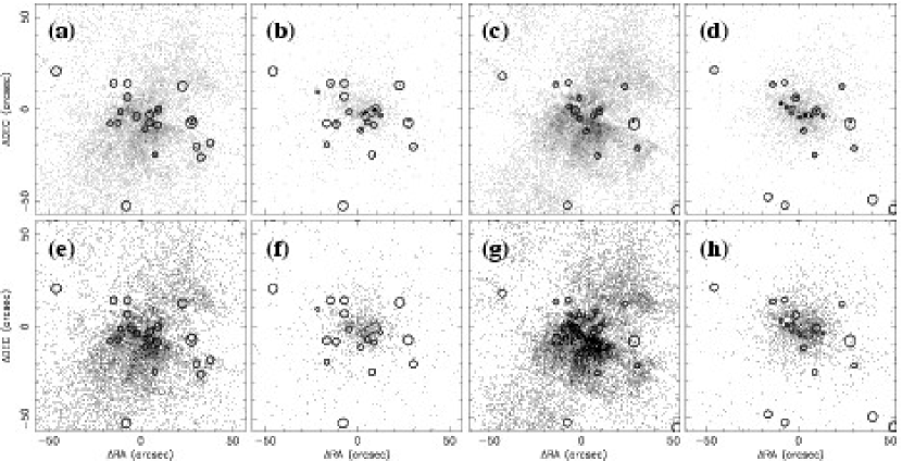
Figure 1.— The center of M82 as seen with Chandra. Each image shows the raw, unsmoothed, photon distribution in the soft 0.3–2.0 keV (panels a and c) and and hard 2.0–8.0 keV energy bands (panels b and d), binned in $0\farcs 492$-wide pixels, over a $2\times 2$ kpc ($1\farcm 90\times 1\farcm 90$) region centered on the dynamical center of the galaxy. Panels a and b are from the ACIS-S observation, while panels c and d are from the merged ACIS-I observation. The images are shown on a square-root intensity scale running from 0 to 75 counts per pixel. Point-like X-ray sources detected in the soft and hard energy bands are shown surrounded by a circle, equivalent in size to the region used to remove the point sources from the images and spectra. Panels e, f, g and h are equivalent to panels a, b, c and d respectively, except that point sources have been removed and interpolated over, and the intensity scale runs from 0 to 25 counts per pixel. The background has been subtracted from all the images in the manner described in § 2.1.3.

2.2. XMM-Newton observations

The two longest XMM-Newton observations of M82 were performed on 2001 May 06 (ObsID 112290201, PI Martin Turner, initial duration 29.4 ks, henceforth referred to as “XMM-short”) and on 2004 April 21 (ObsID 206080101, initial duration 105.4 ks, PI Piero Ranalli, which we shall refer to as “XMM-long”). We did not use a shorter observation ($\sim 10$ ks) taken on the same date as the XMM-short observation because of the low S/N of the resulting spectra.

We reprocessed the archived data using version 6.5 of the XMM-Newton SAS software, and reran the EPIC MOS and PN analysis chains with the latest calibration data. The recommended standard event grade filters and proton flare screening was applied to each dataset. After filtering the remaining exposure times in the XMM-short observation were 21.1 ks and 29.4 ks for PN and each MOS instruments respectively, and in the XMM-long observation 54.0 ks and 72.8 ks for the PN and each MOS detectors respectively.

Spectra and response files were created using SAS using the methods described in the on-line SAS Data Analysis Threads.

Nuclear-region spectra were extracted from the same area used for the Chandra ACIS spectra (see § 4.1). Background spectra for each observation were accumulated in regions of radius $1\farcm 25$ that were free of point sources or diffuse X-ray emission. The same background region was used for all three detectors (PN, MOS1 and MOS2) and whenever possible was on the same CCD chip as the nuclear diffuse emission.

3. Image analysis of the Chandra data

3.1. The spatial distribution of the diffuse soft and hard X-ray emission

The spatial distribution of the soft and hard X-ray emission within $\sim 1$ kpc of the center of M82 as seen in the ACIS-S and merged ACIS-I observations is shown in Fig. 1. Point-like sources identified within each observation are enclosed by circular or rectangular apertures. The only significant differences between the ACIS-S and ACIS-I images are changes in the brightness of some of the point-like X-ray sources due to intrinsic variability, and drops in the apparent diffuse soft X-ray surface brightness in the bottom and top left of the ACIS-I image due to the gaps between the CCD chips.

Images with the point-sources removed are shown in panels e to f of Fig. 1, and were created by replacing events within the point source regions by a Poissonian random deviate consistent with the events detected within a local background annulus of width $1\farcs 5$ around each source-region (CIAO task dmfilth run in POISSON mode). Care was taken to ensure that these background regions did not themselves include any other point source emission. This source removal method is performed on each image. Images in an energy band $<3$ keV have had the point sources removed that were detected only in the soft $E=0.3$–2.0 keV energy band, as sources detected only within the hard $E=2.0$–8.0 keV energy band are most likely heavily obscured and hence invisible at lower energies. Hard X-ray images are cleared of point sources detected in either of the soft or hard X-ray bands. This method produces a source-subtracted image of the 33ks ACIS-I data that is essentially identical that from the PSF-fitting and subtraction method presented in Griffiths et al. (2000).

A more detailed break down of the spatial distribution of the diffuse X-ray emission within the central 2 kpc of M82 as a function of photon energy is shown in Fig. 2, based on the ACIS-S data alone. For comparison we also plot ground-based optical R-band and continuum-subtracted H$\alpha$+[N II] images of the same region.

The effect of absorption by material between us and in the X-ray emitting plasma near the plane of the galaxy is visible at X-ray energies $E<1.1$ keV as a band of low X-ray surface-brightness bisecting the wind from north east to south west, obscuring the nuclear starburst region. This X-ray absorption band has a larger minor-axis extent than the narrower dust lanes seen in the optical images shown in Fig. 2.

At X-ray energies $E\lesssim 0.6$ keV (at energies around the E=0.57 O VII and 0.65 keV O VIII emission lines) the central region of the galaxy is heavily obscured, and the brightness of the diffuse X-ray emission peaks at $z\gtrsim 20\arcsec$ ($\sim 400$ pc) from the mid-plane. In contrast the mid-plane, nucleus and the inner wind are visible in emission from Helium and Hydrogen-like ions of Magnesium ($E\sim 1.3$ – 1.5 keV, where the similarity in morphology to the H$\alpha$+[N II] emission is striking) and Silicon ($E\sim 1.8$ to 2.0 keV), and the brightest emission occurs within $z\sim 50$ pc of the mid-plane. Read & Stevens (2002) and Origlia et al. (2004) studied the nuclear-region element abundance (within $\sim 15\arcsec$ radius of the center of the galaxy) using XMM-Newton RGS grating data. The Origlia et al. study derived a hot-phase Oxygen abundance that is unusually low compared to other $\alpha$-elements. Neither study could take account of the strong spatial variations in foreground absorption within this region (because of the low spatial resolution of XMM-Newton), which our Chandra data shows to be of particular significance in M82 at energies near the oxygen lines. Fitting simple models to spectra with intrinsically complex absorption is known to lead to systematic errors in deriving X-ray abundances from CCD-resolution X-ray spectra (Weaver et al., 2000). We therefor suspect that the abundances derived from XMM-Newton studies of M82 in the Read & Stevens (2002) and Origlia et al. (2004), in particular the apparently low Oxygen abundance, are incorrect.

Diffuse hard X-ray emission is clearly visible within the central starburst region, even in images without point source subtraction. Unlike the diffuse soft X-ray emission from the superwind, the spatial extent of the brightest region of diffuse hard X-ray emission is larger along major axis (i.e. along the plane of the galaxy) than along the minor axis. Measured by eye, hard diffuse X-ray emission has a major-axis radial extent of $\sim 20\arcsec$ ($\sim 350$ pc) approximately centered on the dynamical center of the galaxy, and extends $\sim 8\arcsec$ ($\sim 140$ pc) and $\sim 12\arcsec$ ($\sim 210$ pc) above and below the plane of the galaxy (to the south east and north west of the plane, respectively). Note that diffuse hard X-ray emission can be found outside this central region, although at lower surface brightness. This is discussed further in § 3.3.

The spatial distribution of the diffuse hard X-ray emission is relatively smooth. This is not a limitation of spatial resolution, photon statistics or the method of point source removal, as significant structure is visible in the soft X-ray images. This suggests that the source of the hard X-ray emitting material is also relatively uniformly distributed within the starburst region.

There are three bright point-like X-ray sources just to the west of the center of the galaxy in the ACIS-S and ACIS-I observations (one of which is the variable ultra-luminous X-ray source described in Kaaret et al. 2001; Matsumoto et al. 2001). Point-source removal is difficult in this region, as bright sources have large PSF wings. Combined with the close proximity of these sources to each other we were forced to use a $10\farcs 8\times 4\farcs 4$ rectangular region for point source removal. The flux at each pixel within this region in the source-subtracted images is a Poisson random deviate drawn from the distribution of the fluxes within $1\farcs 5$ of the edge of this rectangle, which includes the region of brightest diffuse hard X-ray emission at the mid-plane of the disk. This method is likely to slightly over-estimate the diffuse X-ray surface brightness at the off-plane location of the ULX, as this entire region is filled in by dmfilth approximately uniformly. Thus the apparent association between the ULX and a bright region of diffuse hard X-ray emission extending off the bright mid-plane ridge (e.g. seen in Fig. 2h) may not be real.

Table 2Count rates and diffuse emission fractions.

Energy	$R_{\rm tot}$	$R_{\rm diff}$	$R_{\rm ps}$	$R_{\rm bg}$	$f_{\rm diff}$	$f_{\rm diff}^{T}$
(keV)	(cts/s)	(cts/s)	(cts/s)	(cts/s)	$\cdots$	$\cdots$
(1)	(2)	(3)	(4)	(5)	(6)	(7)
ACIS-S observation (S3 chip)
0.3 – 0.6	$0.0208\pm{0.0012}$	$0.0191\pm{0.0011}$	$0.0017\pm{0.0004}$	$0.00089\pm{0.00005}$	$0.917\pm{0.203}$	$0.91\pm{0.20}$
0.6 – 1.1	$0.5603\pm{0.0057}$	$0.5263\pm{0.0055}$	$0.0340\pm{0.0014}$	$0.00051\pm{0.00004}$	$0.939\pm{0.041}$	$0.93\pm{0.05}$
1.1 – 1.6	$0.4783\pm{0.0052}$	$0.4347\pm{0.0050}$	$0.0437\pm{0.0016}$	$0.00030\pm{0.00003}$	$0.909\pm{0.035}$	$0.90\pm{0.04}$
1.6 – 2.2	$0.3298\pm{0.0044}$	$0.2727\pm{0.0040}$	$0.0571\pm{0.0018}$	$0.00057\pm{0.00004}$	$0.827\pm{0.029}$	$0.81\pm{0.04}$
2.2 – 2.8	$0.1256\pm{0.0027}$	$0.0901\pm{0.0023}$	$0.0356\pm{0.0015}$	$0.00025\pm{0.00003}$	$0.717\pm{0.033}$	$0.69\pm{0.04}$
0.3 – 2.8	$1.5149\pm{0.0093}$	$1.3429\pm{0.0087}$	$0.1721\pm{0.0032}$	$0.00252\pm{0.00008}$	$0.886\pm{0.017}$	$0.87\pm{0.03}$
5.0 – 6.0	$0.0485\pm{0.0017}$	$0.0138\pm{0.0009}$	$0.0347\pm{0.0014}$	$0.00037\pm{0.00003}$	$0.284\pm{0.015}$	$0.20\pm{0.01}$
6.0 – 7.0	$0.0289\pm{0.0013}$	$0.0079\pm{0.0007}$	$0.0210\pm{0.0011}$	$0.00041\pm{0.00003}$	$0.274\pm{0.020}$	$0.19\pm{0.02}$
3.0 – 9.9	$0.3166\pm{0.0043}$	$0.1071\pm{0.0026}$	$0.2095\pm{0.0035}$	$0.00548\pm{0.00011}$	$0.338\pm{0.007}$	$0.26\pm{0.01}$
Merged ACIS-I data (I3 chip)
0.3 – 0.6	$0.0085\pm{0.0005}$	$0.0082\pm{0.0005}$	$0.0004\pm{0.0001}$	$0.00035\pm{0.00011}$	$0.956\pm{0.288}$	$0.95\pm{0.23}$
0.6 – 1.1	$0.3252\pm{0.0026}$	$0.3172\pm{0.0026}$	$0.0080\pm{0.0004}$	$0.00038\pm{0.00011}$	$0.975\pm{0.053}$	$0.97\pm{0.06}$
1.1 – 1.6	$0.3773\pm{0.0028}$	$0.3447\pm{0.0027}$	$0.0326\pm{0.0008}$	$0.00022\pm{0.00009}$	$0.914\pm{0.025}$	$0.91\pm{0.04}$
1.6 – 2.2	$0.2276\pm{0.0022}$	$0.1877\pm{0.0020}$	$0.0398\pm{0.0009}$	$0.00025\pm{0.00010}$	$0.825\pm{0.021}$	$0.81\pm{0.03}$
2.2 – 2.8	$0.0949\pm{0.0014}$	$0.0691\pm{0.0012}$	$0.0258\pm{0.0008}$	$0.00020\pm{0.00009}$	$0.728\pm{0.024}$	$0.71\pm{0.03}$
0.3 – 2.8	$1.0336\pm{0.0047}$	$0.9269\pm{0.0044}$	$0.1067\pm{0.0015}$	$0.00141\pm{0.00019}$	$0.897\pm{0.013}$	$0.89\pm{0.03}$
5.0 – 6.0	$0.0405\pm{0.0009}$	$0.0101\pm{0.0005}$	$0.0305\pm{0.0008}$	$0.00024\pm{0.00009}$	$0.249\pm{0.009}$	$0.20\pm{0.01}$
6.0 – 7.0	$0.0233\pm{0.0007}$	$0.0063\pm{0.0004}$	$0.0170\pm{0.0006}$	$0.00024\pm{0.00009}$	$0.269\pm{0.013}$	$0.22\pm{0.01}$
3.0 – 9.9	$0.2473\pm{0.0023}$	$0.0830\pm{0.0014}$	$0.1644\pm{0.0019}$	$0.00212\pm{0.00023}$	$0.335\pm{0.005}$	$0.29\pm{0.01}$

Note. — Column 1: Energy band associated with the following count rates. Columns 2, 3 and 4: Background-subtracted count rate within a $0\farcm 476$ radius of 09:55:51.9, +69:40:47.1 (J2000.0). The total background-subtracted count rate (including both diffuse emission and point sources) is $R_{\rm tot}$, while $R_{\rm diff}$ and $R_{\rm ps}$ are the count rates associated with diffuse and point-source emission respectively. Column 5: The background count rate within the same region (see § 2.1.3). Column 6: The apparent diffuse fraction $f_{\rm diff}=R_{\rm diff}/R_{\rm tot}$. Column 7. The diffuse fraction after correcting for unresolved point sources, assuming $x_{r}=0.90$ for the ACIS-S observation and $x_{r}=0.94$ for the merged ACIS-I observation. See § 3.2 for further details. The errors quoted in columns 2 – 6 are $1\sigma$ statistical uncertainties, while the error quoted in column 7 is the combination of the statistical uncertainty in $f_{\rm diff}$ and an assumed 3% uncertainty in $x_{r}$.

3.2. Diffuse emission and unresolved point sources

Count rates for the diffuse emission and the detected point sources within 500 pc of the center of M82 are given in Table 2 for both the ACIS-S and merged ACIS-I observations (the results for the 33 ks ACIS-I observation are consistent with the merged observations). The diffuse count rates are based on the point-source removal technique described above. The point source count rate within any energy band is the difference between the total count rate and the estimated diffuse count rate.

The fraction of the X-ray counts within each energy band from apparently diffuse emission, the diffuse fraction $f_{\rm diff}$, is also presented in Table 2. Some fraction of the apparently diffuse emission comes from unresolved point sources, as only the members of the M82 X-ray source population with individual luminosities $L_{\rm X}\gtrsim 4\times 10^{36}$ erg s^-1 are detected as point-like in these observations (Strickland et al., 2004). Star forming galaxies typically have X-ray point source populations with cumulative luminosity functions of the form $N(>L)\propto L^{-\gamma}$, where $\gamma<1$ (Colbert et al., 2004), i.e. the total luminosity is dominated by the brightest sources. Thus the ratio of the total luminosity in detected point sources to the total luminosity from all point sources is $x_{r}\approx 1-(L_{\rm min}/L_{\rm max})^{1-\gamma}$. Here $L_{\rm min}$ and $L_{\rm max}$ are the luminosities of the faintest and brightest point sources detected. Using this to correct the diffuse fraction for the expected unresolved point source contribution we obtain an estimate of the true diffuse emission fraction $f_{\rm diff}^{\rm T}=1-(1-f_{\rm diff})/x_{r}$. We used a variety of methods to estimate $x_{r}$ in the ACIS-S and ACIS-I observations of M82, where the faintest point sources detected in any energy band typically have $\gtrsim 10$ counts, and the brightest source is the ULX with several thousand counts. We found that for M82 $x_{r}$ depends only weakly on the energy band considered, and the largest effect is the assumed luminosity function slope. We used two values for the slope $\gamma=0.50$ (Kilgard et al., 2003) and $\gamma=0.57$ (Colbert et al., 2004), deriving estimates of $x_{r}$ in the range 0.87 – 0.93 for the ACIS-S observation, and $x_{r}$ in the range 0.91 – 0.96 for the deeper merged ACIS-I observation.

Correcting $f_{\rm diff}$ for unresolved point sources has little effect at energies below $E\sim 3$ keV, but is a non-negligible correction at higher energies. Nevertheless, significant residual diffuse hard X-ray emission exists even after correcting for unresolved point sources, with a fraction $\gtrsim$ 70 % ($f_{\rm diff}^{T}/f_{\rm diff}$) of the apparent diffuse hard X-ray emission being unattributable to unresolved point sources.

In general the estimated diffuse fraction is consistent between the ACIS-S and ACIS-I observations, despite the differences in spectral sensitivity between the back-illuminated and front illuminated chips, and the different epochs of observation. Note that the diffuse fraction is likely to vary with time, in particular in the harder X-ray bands ($E>3$ keV) as significant variability is associated with the nuclear X-ray point sources (e.g.  Collura et al., 1994; Ptak & Griffiths, 1999; Matsumoto & Tsuru, 1999; Matsumoto et al., 2001; Kaaret et al., 2001). Several of the point-like X-ray source did show minor variability in flux between the ACIS-I and ACIS-S observations (as can be seen in Fig. 1), but this was not of a magnitude sufficient to significantly alter the diffuse fraction.

The diffuse fraction is high ($f^{T}_{\rm diff}\geq 70$%) at energies $E\lesssim 3$ keV, but is relatively constant with energy at higher energies ($E\gtrsim 3$ keV) at a value of $f^{T}_{\rm diff}\sim 20$ – 30%. This transition in diffuse fraction occurs at the same energy associated with the transition from X-ray emission extended preferentially along the minor-axis (the soft X-ray emission in the wind) to predominantly major-axis extended hard diffuse X-ray emission shown in Fig. 2.

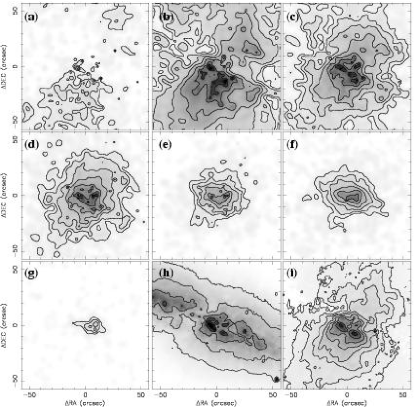
Figure 2.— The distribution of diffuse X-ray emission in the central $2\times 2$ kpc of M82 as a function of energy is shown in panels a to g, compared to optical R-band continuum and continuum-subtracted H$\alpha$+[N II] emission in panels h and i. The energy bands used are E=0.3–0.6 keV (a), 0.6–1.1 keV (b), 1.1–1.6 keV (c), 1.6–2.2 keV (d), 2.2–2.8 keV (e), 3.0–7.0 keV (f) and 6.0-7.0 keV (g). All images are shown on a square root intensity scale. Contour levels increase in factors of 2 in surface brightness. Images are aligned so that North is up and East is to the left. The X-ray images are from the ACIS-S observation, have had background and point source emission removed, and have been adaptively smoothed so that features are locally significant at S/N=3. The intensity scale for the X-ray images runs from 0 to 5 counts (per $0\farcs 492$ pixel), and the contours begin at a level of 0.04 counts per pixel. The effect of strong absorption in the plane of the galaxy is visible at X-ray energies $<1.1$ keV as a band bisecting the wind from north east to south west, obscuring the nuclear starburst region.

Although the ULX is the single brightest X-ray point source over the 0.3–8.0 keV energy band, it accounts for somewhat less than half of the total resolved point source related flux from the central kiloparsec of M82 in either Chandra ACIS observation. In the merged ACIS-I observations of 1999 September 20, the ULX contributed $\sim 51$% of the 0.3–2.8 keV energy band count rate, $\sim 41$% of the 3.0–9.9 keV band count rate and $\sim 45$% of the 0.3-9.9 keV band count rate within a radius of $29\arcsec$ of the center of the galaxy. In the ACIS-S observation of 2002 June 18 the corresponding numbers are 19, 39 and 30% respectively. We estimate that the true count rate of the ULX is probably 50% higher than the observed count rate in the soft energy band, and 20% higher in the hard energy band, due to the effects of pile-up in the ACIS CCD detectors (based on the PIMMS count rate prediction tool), but this does not alter the general conclusion that in total the other resolved point sources contribute a comparable flux to that of the ULX at the specified epochs.

3.3. The spatial extent of the diffuse hard X-ray emission

We created surface brightness profiles along the major and minor axes of the galaxy in several different energy bands in order to better quantify the spatial extent of the diffuse hard X-ray emission in M82, particularly in comparison to the better studied diffuse soft X-ray emission. We also calculated the spectral hardness $Q=(H-S)/(H+S)$, where $H$ and $S$ are the counts in chosen hard and soft energy bands respectively, along these axes. Only data within ${48}\arcsec$ (${835}$ pc) of the respective axis was used when creating each profile in order to achieve a reasonable balance between maximizing the number of counts without averaging over too large an area. We re-binned each profile so as to achieve $\geq 20$ counts per bin per energy band for plotting and fitting the surface brightness profiles, and $\geq 40$ counts per bin per energy band when calculating the spectral hardness. The resulting profiles for the merged ACIS-I observation is are shown in Fig. 3. The ACIS-S surface brightness profiles are in general very similar to the ACIS-I profiles shown in this figure. The most notable differences are purely instrumental due to the effects of the gaps between the ACIS-I CCD chips (at $z\sim-600$ pc and $r\sim-400$ pc). At photon energies $E\gtrsim 1$ keV all profiles show a central peak in emission, the surface brightness of which drops off rapidly with distance, surrounded by more-extended lower surface brightness X-ray emission.

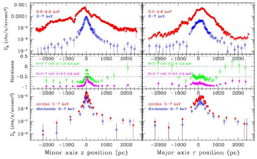
Figure 3.— Minor and major axis diffuse X-ray emission surface brightness and spectral hardness profiles, from the merged ACIS-I observation. The positive $z$ axis is along $PA=343\arcdeg$, and the positive $r$ axis along $PA=253\arcdeg$. The background (§ 2.1.3) has been removed, and point sources interpolated over. Error bars are $1\sigma$ uncertainties. The spectral hardness ratio is defined as $Q=(H-S)/(H+S)$, where $H$ and $S$ are the counts in the higher and lower energy bands respectively.

Along both major and minor axes the hardness ratios show that the emission within $\lesssim 400$ pc of the center of the galaxy is spectrally distinct from the kiloparsec scale emission. The effect of absorption by the disk is seen most clearly in the minor axis hardness ratios. Along the minor axis this hardness ratio drops from the nuclear starburst region to the larger scale wind. Moving to the SE along the wind the hardness is relatively constant in both the ACIS-S and ACIS-I data, although in contrast the hardness ratio increases moving NW from the nucleus.

Simple model fitting demonstrates that to first order the scale heights of the soft and hard diffuse X-ray surface brightness outside the nuclear region are very similar, $H\sim 500$ – 1000 pc. A particularly interesting result is the apparent detection of diffuse hard X-ray emission out to larger $z$ and $r$ distances than recognized in the Griffiths et al. (2000) analysis of the initial ACIS-I observations (out to $|z|\sim|r|\sim 2$ kpc). However this faint extended hard emission X-ray might be due to the extended wings of the Chandra point spread function, rather than being genuinely diffuse emission. We will investigate this issue further in the future.

3.4. Comparison to features at other wavelengths

It is instructive to compare the spatial distribution of the soft and hard X-ray within the central region of M82 to starburst-related activity seen at other wavelengths. In Fig. 4 we plot the location of the near-IR super-star clusters (McCrady et al., 2003), the radio SNRs (Unger et al., 1984; Kronberg & Sramek, 1985; Muxlow et al., 1994; Wills et al., 1998), and the expanding shells seen described in Hi (Wills et al., 2002) and CO-emission (Neininger et al., 1998; Weiß et al., 1999; Matsushita et al., 2000).

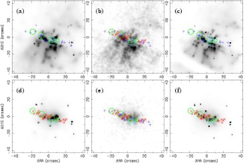
Figure 4.— The X-ray emission from the central $1.5\times 1.5$ kpc region of M82 is shown in comparison to the near-IR super-star clusters of McCrady et al. (2003, small blue crosses), the radio SNRs of Wills et al. (1998, red X’s), the Hi shells described in Wills et al. (2002, shown as blue circles of diameter equivalent to the observed shell) and the CO-superbubble (Weiß et al., 1999, cyan polygon). Panels a and b show ACIS-S images in the $E=0.3$–2.0 keV energy band, including the point source emission in (a) and source-subtracted in (b). Adaptive smoothing has been used in (a), whereas in (b) the smoothing used a Gaussian mask of FWHM$=2\arcsec$. Panel (c) is equivalent to (a), but shows the merged ACIS-I image. Panels (d) through (f) are equivalent to panels (a) through (c), except the images are in the 2.0 – 8.0 keV energy band.

Matsumoto et al. (2001) discuss the relationship between the X-ray point sources seen in the Chandra High Resolution Camera observations of M82 and the 23 radio sources seen at 5 GHz presented in Muxlow et al. (1994). The coordinates of the X-ray point sources seen in both our re-processed ACIS observations and the published HRC observations match within the uncertainties. In Fig. 4 we plot the locations of the 33 compact radio sources observed at 1.4 GHz by Wills et al. (1998). The clearest association of an X-ray source with a radio source at either 1.4 or 5 GHz is with the enigmatic radio source 41.9+58, one of the few radio sources in M82 that is fading with time (Kronberg et al., 2000). The radio source 44.0+59.6, another of the brightest radio sources, falls at the location of a weaker hard X-ray point source. In general the radio sources, most of which are young SNRs evolving in confining dense gaseous environments (Kronberg et al., 2000; Chevalier & Fransson, 2001), are not associated with X-ray point sources.

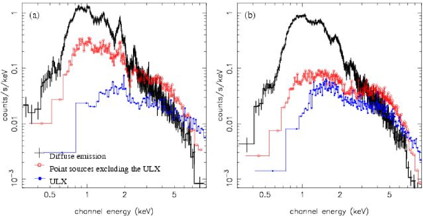
Figure 5.— Background-subtracted ACIS spectra of the nuclear diffuse emission, the summed nuclear point sources (excluding the ULX), and the ULX itself as seen in the ACIS-S observation (a) and the merged ACIS-I observations (b). To improve the clarity of the figure the error bars are not shown on the point source and ULX spectra. The primary differences between the ACIS-S and ACIS-I spectra are purely instrumental, and are due to the poorer low energy sensitivity and spectral resolution of the cosmic-ray-damaged ACIS-I detectors.

Although the SNRs associated with radio sources may not directly contribute to the mechanical powering of the superwind because of their confinement, they must delineate the region associated with current SN activity. It is noteworthy that the major-axis extent of both the soft and hard diffuse X-ray emission is so similar to that of the radio sources — this is the unambiguous sign of a massive-star-related SN-driven wind. The distribution of the diffuse hard X-ray emission differs from that of the radio sources only in that it has a larger minor-axis extent, to be expected if the X-ray-emitting plasma is being advected out along the minor axis.

The near-IR star clusters defined in McCrady et al. (2003) are more widely distributed along the major axis of the galaxy than the radio sources or the soft and hard diffuse X-ray emission. However not all of these clusters are young enough to support ongoing core-collapse SN activity. It is not surprising that there is very little diffuse X-ray emission in the vicinity of the $60\pm{20}$ Myr-old super star cluster F (Smith & Gallagher, 2001). One of the point-like X-ray sources may be associated with the nearby cluster L.

Three of the four expanding Hi shells identified by Wills et al. (2002) lie within the region covered by diffuse soft and hard X-ray emission. As mentioned previously, one of these Hi shells is probably associated with the CO-bubble discussed in Weiß et al. (1999) and Matsushita et al. (2000). This entire region along the major axis is the location of the brightest soft and hard diffuse X-ray emission, there being no discernible difference in X-ray surface brightness between the regions interior and exterior to the Hi and/or CO shells.

4. Spectral analysis of the Chandra and XMM-Newton data

We will begin with an analysis of the Chandra ACIS-S and ACIS-I spectra of each of the diffuse, point source and ULX spectra, followed by assessment of the significance of the $E\sim 6.4$ keV and $E\sim 6.7$ keV iron line features in those spectra. We will then present a more elaborate model that attempts to account for the presence of unresolved point source emission in the diffuse spectrum, and assess what limits can be placed on $E=6.97$ keV emission from hydrogen-like ionized iron in the Chandra spectra. This section is concluded with analysis of the integrated nuclear spectra as seen in the two separated XMM-Newton observations (by integrated we mean that the spectra include diffuse, point source and ULX emission). We will show that a full picture of the origin of the iron line emission from M82 is only obtained if the data from both Chandra and XMM-Newton at all epochs is assessed.

The Chandra ACIS spectra of the central kiloparsec of M82 are quite complex, particularly in the soft X-ray band, where spatially-varying absorption and possible variations in mean plasma temperature occur (see Fig. 5). With the $\Delta E\sim 0.1$ keV resolution of the ACIS-I and ACIS-S CCD detectors the strong line emission from O, Fe, Ne, Mg, Si, and S are heavily blended, making a unique and physically accurate spectral fit currently difficult. Our focus in this paper is instead on the harder X-ray emission with energies $E\gtrsim 2$ keV, where there are fewer spectral features and absorption can effectively be ignored. In particular we are interested in the continuum spectral shape of the diffuse hard X-ray emission, and whether it is similar to that of the resolved point source population. Given the ambiguous detection of iron line emission in the Griffiths et al. (2000) study, another question we wish to answer is what are the statistical significances and fluxes of any $E\sim 6.4$, 6.7 or 6.9 keV iron line emission from the diffuse component? Is the Fe-K emission associated with the point source population, and/or the enigmatic luminous and variable ULX, as Strohmayer & Mushotzky (2003) conclude based on the ObsID 112290201 XMM-Newton observation of M82?

4.1. Chandra ACIS spectra

We extracted spectra from the ACIS-S and ACIS-I datasets within a radius of $28\farcs 6$ (equivalent to a physical radius of 500 pc) of the dynamical center of M82 at $\alpha=09^{\rm h}55^{\rm m}51\fs 9,\delta=+69\arcdeg 40\arcmin 47\farcs 1$ (J2000.0). We extracted and fit spectra to both the merged ACIS-I observation (which has the greatest number of counts) and the 33ks ACIS-I observation (the observation used by Griffiths et al. 2000). A spectrum of the diffuse X-ray emission was created by excluding all detected point sources using either circular or rectangular masks, as shown in Fig. 1. The source extraction radius used depended on source flux, and ranged from $1\farcs 2$ to $3\farcs 0$, most typically being $1\farcs 5$ – $2\arcsec$. These radii were chosen to maximize the removal of point-source related flux from the diffuse spectrum: a radius of $1\farcs 5$ encloses $\sim 85$ – 97% of the flux from a point source, depending on the energy of the photons (the enclosed energy fraction is smaller at higher energies). We also created a summed spectrum of the point source population (excluding the ULX) using these point source extraction regions, and a spectrum of the ULX itself. A small component of the point source and ULX spectra is from truly diffuse emission within the extraction regions. The spectrum of the ULX suffers from “pile-up,” in which two or more X-ray photons arrive in a single pixel within a single 3.2s ACIS exposure and are falsely detected as a single photon of higher energy. We do not seek to correct for this process, but merely to see if any Fe-K line emission can be detected above the local continuum.

We only fit the ACIS spectra in the energy range $E=3.15$ –3.80 keV and $4.20$ – 9.0 keV. Excluding the data below 3.15 keV removes any contribution from the soft diffuse emission and associated Si and S emission, as well as the instrumental Ir edges. We exclude the energy range 3.8-4.2 keV to avoid any He-like and H-like Calcium emission, which is present at marginal significance in the ACIS-S diffuse emission spectrum but is not obvious in the ACIS-I spectra. Our aim is to simplify the spectral fitting by essentially only considering a pure continuum plus any iron lines.

When modeling the continuum in the diffuse and point source spectra we found that standard thermal bremsstrahlung and power law models were adequate. The spectra of the ULX are heavily piled up, and can not be adequately fit with power law or bremsstrahlung models (even when we also included the “pileup” model available in XSPEC). We found that a simple broken power law model, with the transition between the two power law slopes occurring at $E\sim 6.0\pm 0.5$ keV, provided the best fit the the apparent continuum in the ULX spectra. No absorption model was used, as a column $\hbox{$N_{\rm H}$}\sim 10^{23}$ is required to produce an optical depth of $\tau\sim 1$ at $E\sim 3$ keV.

At the spectral resolution of ACIS-S and ACIS-I the Fe-K$\alpha$ fluorescence lines from nearly neutral iron and the Fe He$\alpha$ line complex from highly ionized iron can be modeled as narrow Gaussian ($\sigma=1$ eV) lines at $E=6.40$ and $E=$6.69 keV respectively. Although it is possible to fit the ACIS spectra to determine the the line energy and/or width this does not place any useful constraint on these parameters, nor does this result in statistically superior fits compared to models using the expected line width and energy (by statistically superior we mean a change in chi-squared per change in degrees of freedom $\Delta\chi^{2}/\Delta\nu\geq 1$). For example, when fitting for the line energy of the Fe He$\alpha$ line the best fits were $E=6.66^{+0.10}_{-0.11}$ keV (ACIS-S) and $E=6.69\pm{0.17}$ keV (merged ACIS-I spectrum). Thus for the majority of the spectral fits described below, the line energies and widths were fixed at the expected values, and we fit only for each line intensity.

Table 3Model fits to the diffuse, point source and ULX spectra

Model	Dataset	Continuum model		6.4 keV Fe K$\alpha$ line		6.7 keV Fe He$\alpha$ line		6.9 keV Fe Ly$\alpha$ line		$\chi^{2}$	$\nu$
		$kT$ or $\Gamma$	norm	norm	EW	norm	EW	norm	EW
(1)	(2)	(3)	(4)	(5)	(6)	(7)	(8)	(9)	(10)	(11)	(12)
Chandra diffuse emission spectra
BR, two lines	ACIS-S	$6.2^{+4.7}_{-2.0}$	$9.7^{+2.8}_{-1.9}$	$4.4^{+4.6}_{-4.4}$	112	$8.2^{+5.9}_{-5.9}$	273	$\cdots$	$\cdots$	36.1	81
$\cdots$	33ks ACIS-I	$3.5^{+1.0}_{-0.7}$	$13.0^{+3.5}_{-2.7}$	$5.2^{+4.9}_{-4.9}$	190	$6.3^{+5.4}_{-5.4}$	270	$\cdots$	$\cdots$	65.1	115
$\cdots$	merged ACIS-I	$3.4^{+0.7}_{-0.5}$	$13.6^{+3.0}_{-2.4}$	$5.1^{+4.0}_{-4.0}$	175	$7.7^{+4.6}_{-4.6}$	335	$\cdots$	$\cdots$	94.4	136
BR, no lines	ACIS-S	$8.0^{+8.1}_{-2.8}$	$8.8^{+2.2}_{-1.3}$	$\cdots$	$\cdots$	$\cdots$	$\cdots$	$\cdots$	$\cdots$	43.5	83
$\cdots$	33ks ACIS-I	$4.4^{+1.3}_{-0.9}$	$10.9^{+2.6}_{-1.9}$	$\cdots$	$\cdots$	$\cdots$	$\cdots$	$\cdots$	$\cdots$	77.1	117
$\cdots$	merged ACIS-I	$4.3^{+1.0}_{-0.7}$	$11.3^{+2.2}_{-1.7}$	$\cdots$	$\cdots$	$\cdots$	$\cdots$	$\cdots$	$\cdots$	115.2	138
PL, two lines	ACIS-S	$2.1^{+0.3}_{-0.3}$	$13.7^{+8.7}_{-5.3}$	$4.2^{+4.6}_{-4.2}$	108	$7.9^{+5.8}_{-5.8}$	259	$\cdots$	$\cdots$	34.8	81
$\cdots$	33ks ACIS-I	$2.7^{+0.3}_{-0.3}$	$26.4^{+12.8}_{-8.5}$	$4.9^{+4.9}_{-4.9}$	181	$5.6^{+5.3}_{-5.4}$	232	$\cdots$	$\cdots$	61.0	115
$\cdots$	merged ACIS-I	$2.7^{+0.2}_{-0.2}$	$28.4^{+10.9}_{-7.8}$	$4.8^{+4.0}_{-4.0}$	165	$6.9^{+4.6}_{-4.6}$	293	$\cdots$	$\cdots$	87.2	136
PL, no lines	ACIS-S	$2.0^{+0.3}_{-0.3}$	$11.1^{+6.6}_{-4.1}$	$\cdots$	$\cdots$	$\cdots$	$\cdots$	$\cdots$	$\cdots$	41.9	83
$\cdots$	33ks ACIS-I	$2.5^{+0.3}_{-0.2}$	$20.2^{+8.9}_{-6.1}$	$\cdots$	$\cdots$	$\cdots$	$\cdots$	$\cdots$	$\cdots$	71.4	117
$\cdots$	merged ACIS-I	$2.5^{+0.2}_{-0.2}$	$21.3^{+7.5}_{-5.5}$	$\cdots$	$\cdots$	$\cdots$	$\cdots$	$\cdots$	$\cdots$	105.4	138
BR+PL, three lines	ACIS-S	$3.8^{+2.5}_{-1.2}$	$10.3^{+5.4}_{-3.1}$	$4.4^{+4.6}_{-4.4}$	115	$8.1^{+5.8}_{-5.8}$	253	$1.2^{+4.8}_{-1.2}$	37	35.1	80
$\cdots$	33ks ACIS-I	$2.8^{+0.8}_{-0.5}$	$14.9^{+5.5}_{-3.7}$	$5.4^{+5.2}_{-4.9}$	202	$5.8^{+5.7}_{-5.5}$	235	$0.4^{+5.2}_{-0.4}$	20	63.1	114
$\cdots$	merged ACIS-I	$2.7^{+0.6}_{-0.4}$	$15.7^{+4.6}_{-3.3}$	$5.1^{+4.3}_{-4.0}$	177	$7.4^{+4.5}_{-5.4}$	319	$0.0^{+4.1}_{-0.0}$	0	91.0	135
PL+PL, three lines	ACIS-S	$2.5^{+0.5}_{-0.5}$	$19.1^{+17.8}_{-9.3}$	$4.2^{+4.6}_{-4.2}$	108	$7.8^{+5.8}_{-5.8}$	242	$0.8^{+4.8}_{-0.8}$	24	34.3	80
$\cdots$	33ks ACIS-I	$3.0^{+0.3}_{-0.3}$	$35.1^{+0.4}_{-12.2}$	$4.7^{+4.4}_{-4.7}$	172	$5.5^{+5.0}_{-5.5}$	227	$0.0^{+4.1}_{-0.0}$	0	59.9	114
$\cdots$	merged ACIS-I	$3.0^{+0.3}_{-0.2}$	$37.0^{+20.4}_{-9.9}$	$4.5^{+4.3}_{-3.6}$	154	$6.8^{+4.3}_{-5.0}$	284	$0.0^{+3.1}_{-0.0}$	0	85.1	135
Chandra summed point source spectra, excluding the ULX
PL, two lines	ACIS-S	$1.0^{+0.2}_{-0.2}$	$5.4^{+2.1}_{-1.5}$	$3.2^{+6.6}_{-3.2}$	40	$1.1^{+1.1}_{-7.1}$	13	$\cdots$	$\cdots$	83.0	134
$\cdots$	33ks ACIS-I	$1.0^{+0.2}_{-0.1}$	$4.0^{+1.3}_{-0.7}$	$0.0^{+3.8}_{-0.0}$	0	$3.0^{+4.6}_{-3.0}$	54	$\cdots$	$\cdots$	109.5	166
$\cdots$	merged ACIS-I	$1.0^{+0.1}_{-0.1}$	$3.9^{+0.9}_{-0.7}$	$0.0^{+2.9}_{-0.0}$	0	$4.5^{+5.4}_{-4.5}$	78	$\cdots$	$\cdots$	130.9	206
PL, no lines	ACIS-S	$1.0^{+0.2}_{-0.2}$	$5.2^{+1.9}_{-1.4}$	$\cdots$	$\cdots$	$\cdots$	$\cdots$	$\cdots$	$\cdots$	83.7	136
$\cdots$	33ks ACIS-I	$1.1^{+0.2}_{-0.2}$	$4.1^{+1.1}_{-0.9}$	$\cdots$	$\cdots$	$\cdots$	$\cdots$	$\cdots$	$\cdots$	109.3	168
$\cdots$	merged ACIS-I	$1.0^{+0.1}_{-0.1}$	$3.7^{+8.0}_{-6.6}$	$\cdots$	$\cdots$	$\cdots$	$\cdots$	$\cdots$	$\cdots$	132.5	208
Chandra ULX spectra
BPL, two lines	ACIS-S	$0.3^{+0.4}_{-0.3}$, $-4.5^{+0.9}_{-1.5}$	$0.7^{+0.8}_{-0.4}$	$1.2^{+6.6}_{-1.2}$	19	$0.4^{+7.6}_{-0.4}$	5	$\cdots$	$\cdots$	48.9	89
$\cdots$	33ks ACIS-I	$0.6^{+0.3}_{-0.3}$, $-4.2^{+1.1}_{-1.2}$	$1.1^{+0.8}_{-0.4}$	$1.7^{+5.4}_{-1.7}$	37	$1.2^{+4.1}_{-1.2}$	23	$\cdots$	$\cdots$	71.5	122
$\cdots$	merged ACIS-I	$0.5^{+0.3}_{-0.2}$, $-3.0^{+0.8}_{-1.4}$	$1.0^{+0.5}_{-0.3}$	$0.0^{+4.2}_{-0.0}$	0	$0.0^{+6.4}_{-0.0}$	0	$\cdots$	$\cdots$	103.3	175
BPL, no lines	ACIS-S	$0.3^{+0.4}_{-0.4}$, $-4.5^{+0.6}_{-0.8}$	$0.7^{+0.8}_{-0.7}$	$\cdots$	$\cdots$	$\cdots$	$\cdots$	$\cdots$	$\cdots$	49.0	91
$\cdots$	33ks ACIS-I	$0.6^{+0.3}_{-0.3}$, $-2.6^{+0.9}_{-0.9}$	$1.2^{+0.8}_{-0.5}$	$\cdots$	$\cdots$	$\cdots$	$\cdots$	$\cdots$	$\cdots$	71.5	124
$\cdots$	merged ACIS-I	$0.5^{+0.2}_{-0.2}$, $-3.1^{+1.0}_{-1.0}$	$1.1^{+0.5}_{-0.3}$	$\cdots$	$\cdots$	$\cdots$	$\cdots$	$\cdots$	$\cdots$	103.3	177
XMM-Newton nuclear region spectra including point sources and the ULX
BPL, three lines	XMM-short	$0.7^{+0.1}_{-0.1}$, $2.0^{+0.1}_{-0.1}$	$12.6^{+0.6}_{-0.2}$	$6.6^{+3.7}_{-3.7}$	23	$15.0^{+3.9}_{-2.0}$	58	$6.9^{+3.8}_{-3.9}$	28	1024.9	1555
$\cdots$	XMM-long	$1.6^{+0.1}_{-0.1}$, $2.6^{+0.2}_{-0.2}$	$24.7^{+1.8}_{-1.1}$	$1.3^{+1.5}_{-1.3}$	9	$8.1^{+1.7}_{-1.6}$	70	$0.2^{+1.5}_{-0.2}$	2	1194.6	1573

Note. — All errors are 90% confidence for 1 interesting parameter. Column 1: Abbreviations for the continuum model used, and whether the 6.4 and 6.7 keV lines were fit for. Thermal Bremsstrahlung: BR; Power Law: PL; Broken power law: BPL; Bremsstrahlung with additional power law component representing unresolved X-ray binary emission: BR+PL; Power law with additional power law component representing unresolved X-ray binary emission: PL+PL; The break energy for the BPL model is not tabulated, but ranged from 5.6 to 6.3 keV in the best fit models to both the Chandra and XMM-Newton spectra. The power law component used in the BR+PL and PL+PL models to represent the unresolved X-ray binary emission is described in § 4.2. Column 3: Temperature kT (keV) for bremsstrahlung models, or photon index for power law models. Two photon indexes are given for the broken power law models fit to the ULX. Column 4: Continuum model normalization factor. These values are numerically $10^{4}\times K$, where $K$ is the XSPEC model normalization factors. For the bremsstrahlung models $K=3.02\times 10^{-15}/4\pi D^{2}\times\int n_{e}n_{I}dV$ where $n_{e}$ and $n_{I}$ are the electron and ion number densities respectively (cm^-3), $D$ is the distance to the source in cm and $V$ the volume of the emitting region. For the power law and broken power law models $K$ is the photon flux per unit energy (units of photons/keV/cm²/s), evaluated at $E=1$ keV Columns 5, 7 and 9: Line normalizations, effectively total line flux in units of $10^{-6}$ photons s^-1 cm^-2. Columns 6, 8 and 10: Line equivalent widths corresponding to the best-fit line and continuum normalizations, in units of eV. Column 11: Best-fit $\chi^{2}$ value. Column 12: Total number of degrees of freedom.

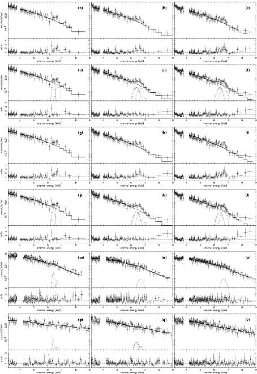
Figure 6.— Nuclear diffuse (panels a – l), point source (excluding the ULX, panels m – o) and ULX spectra (panels p – r) and best-fit models with residuals. The first column are ACIS-S spectra, the second column spectra from the 33ks ACIS-S observation and the third column spectra from the merged ACIS-I observation. Panels a – c and g – i (the first and third rows) are pure power law and bremsstrahlung models respectively, in which residuals in 6.2 – 6.8 keV energy range are clearly visible. Panels d – f and j – l (second and fourth rows) are power law with lines and bremsstrahlung with lines model fits to the diffuse spectra. The point source spectra are shown with best-fit models of a power law plus lines in panels m – o, and the ULX spectra with a broken power law plus lines model in panels p – r. The emission lines in the point source and ULX models are not required statistically.

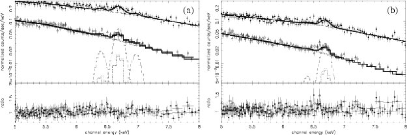
Figure 7.— XMM-Newton spectra of the nuclear region of M82, along with best-fitting models. The shorter of the two observations is shown in panel a, and the longer in panel b. Data from the PN detector is shown as filled black circles, MOS1 data as open triangles and MOS2 data as open squares. The solid, dashed and dotted lines are the best fit model components.

The best-fit spectral models are plotted along with the diffuse, point source and ULX spectra in Fig. 6, and the best-fit model parameters are shown in Table 3. The derived fluxes for the diffuse emission are shown in Table 4. The pure continuum model fits to the diffuse emission spectra (i.e. without any line components) show strong residuals in the energy range 6.2 – 6.8 keV in the ACIS-S, 33ks ACIS-I and merged (48ks) ACIS-I spectra, and the addition of the two lines does a good job of removing these residuals. The addition of the Gaussian model components representing Fe K$\alpha$ and Fe He$\alpha$ emission improves the quality of fit in all the diffuse emission spectra, but not in the point source and ULX spectra. Quantitatively the best-fit $\chi^{2}$ values are reduced by between 7 and 18 for the diffuse spectra, but change by only $\Delta\chi^{2}=-1.6$ to +0.2 in point source spectra, and do not change at all in the ULX spectra.

A power law continuum model gives a marginally better fit to the diffuse emission continuum than a bremsstrahlung model in ACIS-S and ACIS-I spectra, but visual inspection of the best fit models shows that the differences between the two best-fit continuum models are very subtle. It is noteworthy that the slopes of the all of the best fit power law models to the diffuse emission ($2.0\lesssim\Gamma\lesssim 2.7$) are significantly different from the slope of the resolved point source spectra ($\Gamma=1.0\pm{0.2}$). This is further evidence that the bulk of the diffuse hard X-ray emission does not arise in an unresolved population of point sources that are similar to but fainter than the resolved point source population. The power law slopes fit for the ACIS-S and ACIS-I diffuse emission spectra differ at greater than 90% confidence. We will address this issue when we fit the more elaborate models to the diffuse emission in § 4.2.

CCD-resolution X-ray spectra that fit well with a continuum plus weak line feature are often also well-fit by a continuum plus absorption edge model. This model is physically plausible in the case of AGN where there may be very large column densities of absorbing material along the line of sight to the point-like continuum source. In the case of M82 where the apparent line feature is seen in the diffuse X-ray emission that covers a region several hundred parsecs in size an implausible amount of iron would be required in an absorption edge model. We therefor do not consider this case further.

4.1.1 The significance of the iron lines in the diffuse emission spectra

These spectral fits demonstrate the presence of weak line features in the diffuse emission spectra, and very weak or negligible line emission in the point source and ULX spectra. That the ACIS-S and ACIS-I spectra independently yield similar best-fit spectral parameters suggests that these results are not a statistical fluke or calibration oddity. Nevertheless we would like to better quantify the true significance of the Fe line detections in the diffuse emission, and the lack of detection in the point source and ULX spectra.

In X-ray astronomy it has been traditional to use an F-test to assess the significance of the addition of a weak line component to a spectral fit, but Protassov et al. (2002) show that this is inappropriate. We therefor used Monte-Carlo models to assess the significance of the line features in the diffuse and ULX spectra, as well as the uncertainties in the diffuse emission line fluxes.

Table 4Hard X-ray fluxes and luminosities

Dataset	Continuum, 2 – 8 keV)		6.4 keV Fe K$\alpha$ line		6.7 keV Fe He$\alpha$ line		6.9 keV Fe Ly$\alpha$ line
$\cdots$	$f_{X}\times 10^{12}$	$L_{\rm X}\times 10^{-39}$	$f_{X}\times 10^{14}$	$L_{\rm X}\times 10^{-37}$	$f_{X}\times 10^{14}$	$L_{\rm X}\times 10^{-37}$	$f_{X}\times 10^{14}$	$L_{\rm X}\times 10^{-37}$
$\cdots$	${\rm\thinspace erg}{\rm\thinspace s}^{-1}\,$${\rm\thinspace cm}^{-2}\,$	${\rm\thinspace erg}{\rm\thinspace s}^{-1}\,$	${\rm\thinspace erg}{\rm\thinspace s}^{-1}\,$${\rm\thinspace cm}^{-2}\,$	${\rm\thinspace erg}{\rm\thinspace s}^{-1}\,$	${\rm\thinspace erg}{\rm\thinspace s}^{-1}\,$${\rm\thinspace cm}^{-2}\,$	${\rm\thinspace erg}{\rm\thinspace s}^{-1}\,$	${\rm\thinspace erg}{\rm\thinspace s}^{-1}\,$${\rm\thinspace cm}^{-2}\,$	${\rm\thinspace erg}{\rm\thinspace s}^{-1}\,$
(1)	(2)	(3)	(4)	(5)	(6)	(7)	(8)	(9)
ACIS-S	$2.86_{-0.29}^{+0.11}$	$4.43_{-0.45}^{+0.17}$	$5.67_{-3.77}^{+3.77}$	$8.78_{-5.85}^{+5.84}$	$11.00_{-5.02}^{+5.02}$	$17.00_{-7.78}^{+7.78}$	$<9.24$	$<14.3$
33ks ACIS-I	$2.76_{-0.12}^{+0.17}$	$4.28_{-0.26}^{+0.19}$	$5.82_{-3.30}^{+3.74}$	$9.02_{-5.12}^{+5.80}$	$7.11_{-4.37}^{+3.83}$	$11.0_{-6.78}^{+5.95}$	$<7.15$	$<11.1$
Merged ACIS-I	$2.81_{-0.12}^{+0.11}$	$4.35_{-0.19}^{+0.17}$	$5.53_{-2.52}^{+3.32}$	$8.58_{-3.91}^{+5.15}$	$8.73_{-3.77}^{+3.36}$	$13.50_{-5.85}^{+5.22}$	$<6.58$	$<10.2$
XMM-short	$\cdots$	$\cdots$	$6.77_{-2.30}^{+2.26}$	$10.50_{-3.57}^{+3.51}$	$16.10_{-2.54}^{+2.55}$	$24.90_{-3.95}^{+3.95}$	$7.74_{-2.60}^{+2.59}$	$12.0_{-4.04}^{+4.02}$
XMM-long	$\cdots$	$\cdots$	$1.32_{-0.94}^{+0.94}$	$2.04_{-1.45}^{+1.46}$	$8.70_{-1.06}^{+1.10}$	$13.50_{-1.65}^{+1.71}$	$<3.00$	$<4.66$
ULX high state	$\cdots$	$\cdots$	$5.45_{-2.48}^{+2.45}$	$8.45_{-3.85}^{+3.80}$	$7.37_{-2.76}^{+2.78}$	$11.40_{-4.28}^{+4.31}$	$7.47_{-2.62}^{+2.79}$	$11.60_{-4.06}^{+4.33}$

Note. — Fluxes and luminosities quoted refer to the diffuse emission alone for the Chandra ACIS data. The contribution of the unresolved point sources has been removed from these values. Fluxes derived from the XMM-Newton data are the total line fluxes from the nuclear region, which are a combination of the point source and diffuse X-ray emission. No broad-band flux is quoted for the XMM-Newton data as we do not attempt to separate the diffuse the diffuse and point source contributions. The diffuse emission fluxes shown above have been corrected from those derived from the diffuse spectra to account for the diffuse flux in the point source and ULX spectra regions (an increase by a factor 1.32 for the ACIS-S data and 1.20 for both ACIS-I datasets). All errors are 68.3% confidence in one interesting parameter. Upper limits are reported at 99% confidence. Note that the E=2 – 8 keV energy band continuum luminosities do not include the line emission.

We created 40000 realizations of pure-continuum spectra (no lines) using both the ACIS-S and merged ACIS-I dataset best-fit power-law models, and fit them in the same manner as the real data with power law plus line models. We then assessed how often the fit-derived line fluxes in the 6.4 keV, 6.7 keV and summed 6.4 and 6.7 keV lines equaled or exceeded the observed values. We found that we can reject the null hypothesis (that the lines found in the real data are merely noise) at high confidence for all lines in both datasets.

For the weaker of the line features seen in the diffuse emission, the E=6.4 keV line, the null hypothesis can be rejected at 98.6225% confidence for the ACIS-S observation alone, and at 99.9225% confidence for the merged ACIS-I observation considered on its own. The probability that a spurious E=6.4 keV line feature would appear in both sets of observations if there were no line emission at $E=6.4$ and 6.69 keV is essentially negligible.

The null hypothesis can be rejected with even more confidence for the 6.7 keV line feature, at 99.99985% confidence for the ACIS-S data considered alone. In none of the 40000 simulation of the merged ACIS-I data did Poissonian noise create a spurious 6.7 keV line feature with a flux equal to or greater than that observed.

The $E=6.7$ keV Fe line normalization derived from the ACIS-S data is larger than that from the ACIS-I data by a factor of $\sim 1.6$, marginally larger than the $68$% confidence regions. The continuum normalizations also differ in the same sense but by a factor of $1.2$. Accounting for the continuum contribution from unresolved point sources (discussed below) will reduce the differences in spectral shape and normalization between the ACIS-S and ACIS-I spectra.

Table 5Best fitting Fe $He\alpha$ line energies

Dataset	6.4 keV line present?	Fe He$\alpha$ line		Fit statistic
		Centroid (keV)	Width (keV)	$\Delta\chi^{2}$	$\Delta\nu$
(1)	(2)	(3)	(4)	(5)	(6)
ACIS-S	yes	$6.66^{+0.10}_{-0.11}$	(f)	-0.3	-1
$\cdots$	no	$6.66^{+0.10}_{-0.22}$	(f)	1.7	0
$\cdots$	no	$6.61^{+0.14}_{-0.15}$	$0.15^{+0.19}_{-0.15}$	0.2	-1
Merged ACIS-I	yes	$6.69\pm{0.17}$	(f)	-0.1	-1
$\cdots$	no	$6.64^{+0.06}_{-0.22}$	(f)	2.6	0
$\cdots$	no	$6.54^{+0.13}_{-0.15}$	$0.20^{+0.17}_{-0.20}$	0.1	-1
XMM-long	yes	$6.65\pm{0.02}$	(f)	-6.7	-1
$\cdots$	no	$6.65\pm{0.02}$	(f)	-5.4	0
$\cdots$	no	$6.65\pm{0.02}$	$0.07\pm{0.03}$	-9.2	-1
XMM-short	yes	$6.66\pm{0.03}$	(f)	-2.3	-1
$\cdots$	no	$6.66^{+0.03}_{-0.04}$	(f)	5.6	0
$\cdots$	no	$6.63^{+0.09}_{-0.08}$	$0.23^{+0.08}_{-0.07}$	-2.9	-1

Note. — The change in the fit statistic with respect to the best-fit model from Tab 3 if the energy and width of the $E\sim$ 6.7 keV is fit for, and if the $E=6.4$ keV line is present or not. For the Chandra diffuse emission spectra the best-fit model used was the “PL+PL, three lines” model. For the XMM-Newton spectra of the entire nuclear region the best-fit model was the “BPL, three lines” model. Confidence regions correspond to 90% confidence for one interesting parameter. Column 2: Records whether or not a narrow line at $E=6.4$ keV is included in the spectral model. Column 3: The energy of the Fe He$\alpha$ Gaussian line centroid (keV). Column 4: The Gaussian width of the Fe He$\alpha$ Gaussian line (keV). Note that this is $\sigma$, not the FWHM. Models where this width was fixed at the default value 0.001 keV are denoted with “(f)”. Column 5: The change in the best-fit $\chi^{2}$ value from the default model in Table 3. A negative $\Delta\chi^{2}$ indicates a better fit. Column 6: The change in the number of degrees of freedom $\nu$ from the default model.

4.1.2 Is only one of the lines real?

We also considered the possibility that only one of the lines is genuine, and that the other is noise. Considering the case where only the 6.4 keV line was assumed to be genuine, the number of times we found a spurious 6.7 keV line with the observed flux in 10000 simulated spectra was 1 for the ACIS-S data and 0 for the longer merged ACIS-I observation, i.e. this hypothesis can be rejected at $\gtrsim 99.99$% confidence for each of the datasets independently.

The chance that we could mistakenly find a 6.4 keV line feature if there were in reality only a 6.7 keV line feature is not negligible for the ACIS-S data: this hypothesis can only be rejected at 51% confidence. In the higher S/N merged ACIS-I observation this hypothesis can be safely rejected with 99.8% confidence.

Note that these probabilities assume that the lines are intrinsically narrow and are at the expected energies of E=6.4 and 6.69 keV. If we allow the central energy (and optionally the width) of the Gaussian component represent the Fe He$\alpha$ line to vary the statistical significance of the 6.4 keV line feature is reduced. Table 5 shows the best-fit line energies and $\chi^{2}$ values for models fitting for the Fe He$\alpha$ line energy compared to the default spectral fits described above. We also experimented with removing the 6.4 keV line so as to assess whether a single line at $E\neq 6.69$ keV provides as good a fit as two lines at $E=6.4$ and $E=6.69$ keV

For the ACIS diffuse emission spectra fitting for the Fe He$\alpha$ line energy provides essentially negligible improvement in the fit statistic. Removing the 6.4 keV line leads to marginally worse fits ($\Delta\chi^{2}\sim 2$). However a single broader line at $E\sim 6.5$ – 6.6 keV provides as good a fit as two narrow lines at $E=6.4$ and 6.69 keV in both the ACIS-S and merged ACIS-I diffuse emission spectra. The best-fitting line width of $\sigma\sim 0.2\pm{0.2}$ keV is to poorly constrained to be used as a physical constraint on the validity of the model.

Based on purely statistical arguments we can not distinguish between a model for the diffuse nuclear emission with two narrow lines at $E=6.4$ and $E=6.69$ keV and a model with a single broader line at $E\sim 6.6$ keV. We conclude that the evidence for the $E=6.4$ keV iron line in the ACIS diffuse emission spectra is of marginal statistical significance.

4.1.3 Iron lines and the point sources

Including line components in the fits to the summed point source and ULX spectra leads to negligible changes in the best-fit $\chi^{2}$ values. From the existing fits it is safe to assume that there is no significant iron line emission in the spectra of the point sources (excluding the ULX). In the case of the ULX the apparent continuum level in the $E=6$ – 7 keV energy band is significantly higher than in the diffuse or point source spectra. Would such a high continuum make it difficult to see weak iron line emission in the Chandra ACIS spectra, or even miss line fluxes as high as those found in the diffuse emission? For the ULX to be a significant contributor to the total hard X-ray iron line emission from M82 it would have to produce a line luminosity comparable to that from the diffuse emission. We created 10000 simulated spectra of the ULX, again for both ACIS-S and ACIS-I observations, using the best-fit broken power law continuum model along with iron lines equal in flux to those in the best-fit diffuse emission spectra, and then evaluated how often we would have fit line fluxes for the ULX as low we observed. For the ACIS-S this would only tend to happen 15.3, 2.5, and 1.0% of the time, for the 6.4 keV, 6.7 keV and summed line fluxes respectively. The equivalent numbers for the ACIS-I dataset are 2.4, 0.7 and 0.1%.

We conclude that despite the relatively high continuum level in the Chandra ACIS spectra of the ULX we could detect iron lines of comparable flux to that in the diffuse emission spectra with relative ease. That we did not in either set of Chandra observations indicates that the ULX was not a source of significant 6.4 keV or 6.7 keV line emission in September 1999 or June 2002.

Table 6The 6.9 keV line flux and 6.9/6.7 keV line ratio.

Dataset	6.9 keV line norm	6.9/6.7 keV line ratio	$kT_{\rm CIE}$
(1)	(2)	(3)	(4)
ACIS-S	$<6.27$	$<0.80$	$<1.1\times 10^{8}$
33ks ACIS-I	$<5.39$	$<0.97$	$<1.2\times 10^{8}$
Merged ACIS-I	$<4.91$	$<0.72$	$<1.0\times 10^{8}$
XMM-long	$<2.69$	$<0.33$	$<7.6\times 10^{7}$
XMM-short	$6.9\pm{0.23}$	$0.46\pm{0.27}$	$(8.7^{+2.0}_{-2.7})\times 10^{7}$
ULX high state	$6.7\pm{0.39}$	$1.03\pm{0.66}$	$(1.3^{+0.4}_{-0.5})\times 10^{8}$

Note. — Upper limits are reported at 99% confidence. Where two-sided confidence regions are reported they are 68.3% confidence for one interesting parameter. Column 2: Upper limit or best-fit value for the 6.969 keV line normalization, in units of $10^{-6}$ photons s^-1 cm^-2. Column 3: Upper limit or best-fit value for the ratio of the photon flux in the 6.9 keV (Fe Ly$\alpha$) to 6.7 keV (Fe He$\alpha$) lines, Column 4: Upper limit or value for the plasma temperature in Kelvin, derived from the 6.9/6.7 keV line ratio, assuming collisional ionization equilibrium (CIE) and using the APEC plasma code.

4.2. More elaborate fits the Chandra diffuse emission spectra

It is worthwhile to consider two further elaborations of the previously performed spectral fits: accounting for the contribution of unresolved point sources to the continuum spectral shape, and placing limits on the line flux of Hydrogen-like Fe at $E=6.97$ keV.

Based on the diffuse fractions described in § 3.2 we know that a small but non-negligible fraction of the Chandra diffuse spectra is contributed by unresolved point sources (URPS). The fraction of the apparently diffuse count rate in the E=3.0 – 9.9 keV energy band arising in these unresolved sources is $R_{\rm diff-urps}/R_{\rm diff}=1-(f^{\rm T}_{\rm diff}/f_{\rm diff})\sim 0.23$ for the ACIS-S observation and $\sim 0.13$ for the merged ACIS-I observation. The longer exposure time of the merged ACIS-I observation leads to a significant improvement in point source removal, and reduction in spectral contamination by unresolved sources. The power law slope of the summed spectrum of the resolved point sources ($\Gamma\sim 1.0$) is significantly flatter that the fitted diffuse emission continua ($\Gamma\sim 2.1$ (ACIS-S) or 2.7 (ACIS-I)). If the unresolved sources have a similar spectrum to the resolved point sources then accounting for the URPS contribution should steepen the fitted continuum spectral shape of the true diffuse emission.

We modeled the contribution of the URPS to the diffuse spectra as a power law component with the same spectral slope as the resolved point sources, and with a normalization that produces the expected count rate $R_{\rm diff-urps}=(f_{\rm diff}-f^{\rm T}_{\rm diff})\times R_{\rm tot}$ in the 3.0 – 9.9 keV energy band. Given the uncertainties in $f^{\rm T}_{\rm diff}$ and $R_{\rm tot}$ this normalization is accurate to $\sim 5$%. The power law slope and normalization of the URPS component are fixed and are not allowed to vary during the spectral fitting. A Gaussian line component at a fixed energy of $E=6.969$ keV was added to represent the Fe Ly$\alpha$ line. The results of these fits are given in Table 3.

Both bremsstrahlung and power law models were used for the continuum shape of the true diffuse X-ray component, although we found that a power law continuum was still favored statistically over a bremsstrahlung model. The best fit normalization of the 6.9 keV line is often zero and in all cases statistically consistent with zero (although note that the two sided confidence regions reported by XSPEC and given in Table 3 do not strictly apply when the region includes zero. Rigorously derived upper limits on the 6.9 keV line flux are described below).

Best-fit $\chi^{2}$ values are lower (i.e. better) than the simpler models previously discussed, but the improvement is not statistically significant. Nevertheless this exercise is worthwhile in that including the expected contribution from the URPS leads to a closer match between the fitted ACIS-S and ACIS-I diffuse component continuum shape ($\gamma$ or kT).

We used Monte-Carlo simulations (with 5000 realizations each for the ACIS-S, 33ks ACIS-I and merged ACIS-I spectra) to derive upper limits on the 6.9 keV line flux and 6.9/6.7 line flux ratio. Simulations were used to convert the limits on the line flux ratio into limits on the plasma temperature, assuming collisional ionization equilibrium (CIE). These limits are shown in Table 6, and the corresponding line luminosities are given in Table 4.

4.3. XMM spectra

Nuclear region spectra were extracted from both of the XMM-Newton observations within a radius of $28\farcs 6$ of $\alpha=09^{\rm h}55^{\rm m}51\fs 9,\delta=+69\arcdeg 40\arcmin 47\farcs 1$ (J2000.0), the same region as used for the Chandra spectra. It is impossible to separate the nuclear diffuse emission from the point sources and ULX emission with XMM-Newton, so the spectra shown in Fig. 7 represent all the emission from this region. We will not attempt to spectrally-separate the different components of the diffuse hard X-ray continuum, but are interested primarily in the Fe line fluxes and energies: are they consistent with the Chandra ACIS spectra; and can the superior sensitivity of the XMM-Newton spectra be used to detect or place stronger limits on the $E=6.4$ and $E=6.9$ keV line emission?

For each observation the EPIC PN, MOS1 and MOS2 spectra were simultaneously fit with the same spectral model, allowing for minor differences between the PN and MOS calibrations by fitting for a multiplicative term that is applied to the model normalizations (typically the MOS1 and MOS2 model normalizations must be increased by $\sim 5$ – 8% [MOS1] and $\sim 3$% [MOS2]). The spectral data are fit only in the 3.4 – 9.0 keV energy range, and the spectra are rebinned to attain $\geq 10$ counts per bin.

We find that a broken power law provides the best representation of the continuum spectral shape in both XMM-Newton datasets. The best fit spectral parameters are presented in Table 3, the 6.9 keV line flux and 6.9/6.7 keV line ratios in Table 6, and the line luminosities in Table 4.

In the longer XMM-Newton observation (2004 April 21) the $E=6.7$ and 6.9 keV iron line fluxes are very similar to those seen in the Chandra ACIS spectra, although the 6.4 keV line flux is significantly lower in the XMM-Newton spectrum.

Fitting for the energy of the Fe He$\alpha$ line in this dataset results in a significant improvement in the fit at a line centroid energy of $E=6.65\pm{0.02}$ keV (see Table 5). Removing the weak E=6.4 keV Fe K$\alpha$ line results in slightly worse fit, but as with the ACIS diffuse emission spectra we find that the evidence for the presence of $E=6.4$ keV emission is of marginal quality. Once again a broad line (Gaussian $\sigma=0.07\pm{0.03}$ keV, 90% confidence in one parameter) provides a better fit than a narrow Fe He$\alpha$ line. This, if not due to systematic effects in the detector, corresponds to a velocity FWHM $\sim 7400\pm{3200}\hbox{${\rm\thinspace km}{\rm\thinspace s}^{-1}\,$}$ or the thermal line width for $T\sim 7\times 10^{10}$ K iron ions. These values are large compared to the maximum bulk velocities and temperatures expected in thermalized SN ejecta of $v\sim 3000\hbox{${\rm\thinspace km}{\rm\thinspace s}^{-1}\,$}$ and $T\sim 10^{8}$ K (Chevalier & Clegg, 1985), leading us to doubt whether the broadening of the $E\sim 6.65$ keV line is real. Unfortunately the lack of a strong (and intrinsically narrow) 6.4 keV line prevents us from assessing the level of systematic effects (for example as done in Tanaka et al. 2000).

In the XMM-Newton observation of 2001 May 06 the iron line fluxes are considerably larger than seen in any of the ACIS spectra or the longer XMM-Newton observation. Furthermore there is a significant detection of the 6.9 keV line, and the overall hard X-ray continuum is several times brighter than at the epoch of the XMM-long observation. It is most likely that the ULX is responsible for this additional flux, given previous and more extreme hard X-ray variability (Ptak & Griffiths, 1999; Matsumoto & Tsuru, 1999).

Assuming that the iron line flux seen in the longer XMM-Newton observation comes from a non-varying diffuse X-ray component we can calculate the line flux due to the ULX alone in the high state it was in on 2001 May 06. For completeness we present these estimated ULX line fluxes and a temperature estimate from the 6.9/6.7 keV line ratio in Tables 6 & 4, even though they do not pertain to the diffuse emission.

Fitting for the Fe He$\alpha$ line energy in this observation only leads to a marginal improvement in the fit (Table 5). The presence of the 6.4 keV line is strongly favored, if Fe He$\alpha$ is narrow, but as with the other nuclear spectra we have discussed a single broad line at $E\sim 6.6$ keV provides as good a fit as two narrow lines at $E=6.4$ keV and $E=6.69$ keV.

5. Discussion

The multiple Chandra and XMM-Newton observations of M82 provide a relatively self-consistent picture of the diffuse hard X-ray continuum and iron line emission. The emission is brightest within the spatial region associated with the ongoing starburst and supernova activity. Emission at $E\sim 6.7$ keV (the Fe XXV He$\alpha$ line complex) is detected with high statistical significance in all the observations we have analyzed. We can only place upper limits on diffuse $E\sim 6.9$ keV emission (the Fe Ly$\alpha$). The statistical significance of diffuse $E\sim 6.4$ keV emission is marginal in both the diffuse spectra obtained with Chandra and the total nuclear spectra provide by the XMM-Newton observations.

5.1. Iron line emission: previous observations and point sources

These results demonstrate that the iron line emission in M82 comes from a diffuse source and not from compact objects in three of the four epochs sampled by Chandra and XMM-Newton observations. In general the iron line emission from the summed point sources and/or the ULX appears to be of negligible intensity compared to the diffuse iron line emission.

Nevertheless the distinctly higher iron line intensity (in particular at $E=6.9$ keV) seen in the XMM-short observation compared to the relatively consistent iron line intensities seen the in the other Chandra and XMM-Newton observations indicate that compact objects can contribute at times to the iron line emission from M82. It is most likely that the additional iron line emission came from the ULX.

The analysis presented by Strohmayer & Mushotzky (2003), where they assumed that all the iron line emission came from the ULX, was based on this XMM-short observation. With our results we can now separate remove the time-constant diffuse contribution to the total iron line emission in this observation (Table 4). The 6.4 and 6.7 keV iron line fluxes from ULX in this high iron-line-emitting state were comparable to the total diffuse iron line emission. At this epoch the 6.9 keV line emission from the ULX is of comparable intensity to the 6.7 keV emission.

K-shell iron line emission has previously been detected in Ginga, ASCA and BeppoSAX X-ray spectra of M82, although the uncertainties in the mean line energy and flux were large. Ginga observations of M82 (Ohashi et al., 1990; Tsuru, 1992) detected emission at $E\sim 6.7$ keV with an equivalent width of $170\pm{60}$ eV. Ptak et al. (1997) reported a marginally significant ($3\sigma$) detection of a line at $E\sim 6.6$ keV with an equivalent width of 100 eV based on observations with ASCA. Using the same data Tsuru et al. (1997) concluded that evidence for the line was not significant, and gave an upper limit at 99% confidence on the equivalent width of any line in the energy range $6.3\lesssim E$ (keV) $\lesssim 7.1$ of less than 100 eV. Later observations of M82 with ASCA found a variable X-ray source (most probably the ULX) in an extremely luminous state, and in these observations the spectra displayed weak iron line emission with an equivalent width of $121^{+56}_{-61}$ eV (Matsumoto & Tsuru, 1999). Cappi et al. (1999) fit for both Fe K$\alpha$ and Fe He$\alpha$ lines in the BeppoSAX observations of M82, of which only the latter was detected (at $E=6.6\pm{0.2}$ keV) with an equivalent width of $60^{+36}_{-45}$ eV.

These historical values are similar to the range we find in the two XMM-Newton observations, where the total iron line equivalent widths were 109 eV (XMM-short) and 81 eV (XMM-long), although this may be a coincidence. Indeed, based on our results we would expect the iron line equivalent width in M82 to vary, as we know that the total hard X-ray continuum is strongly influenced by the variability associated with point sources, and also that at some epochs (in one of the four observations we analyze) one or more point sources also contribute to the iron line emission.

Cappi et al. (1999) provide Fe He$\alpha$ and Fe K$\alpha$ line photon fluxes and upper limits in their analysis of the BeppoSAX observation of M82 which are consistent with the iron line normalizations we find (Table 3). The most convincing case for $E=6.4$ keV Fe K$\alpha$ emission we have is in XMM-short observation. Here the observed line photon flux was $(6.6\pm{3.7})\times 10^{-6}$ photons ${\rm\thinspace cm}^{-2}\,$ s${}^{-1}\,$, consistent with the upper limit of $<1.5\times 10^{-5}$ photons ${\rm\thinspace cm}^{-2}\,$ s${}^{-1}\,$ in the BeppoSAX observation. The Fe He$\alpha$ line flux is not well constrained in the BeppoSAX data: $(1.6^{+1.1}_{-1.0})\times 10^{-5}$ photons ${\rm\thinspace cm}^{-2}\,$ s${}^{-1}\,$, which is consistent with both the flux from the diffuse emission alone ($\sim 6$ – $8\times 10^{-6}$ photons ${\rm\thinspace cm}^{-2}\,$ s${}^{-1}\,$) or the larger flux of $(1.5^{+0.4}_{-0.2})\times 10^{-5}$ photons ${\rm\thinspace cm}^{-2}\,$ s${}^{-1}\,$ in the XMM-short observation.

Even in Chandra and XMM-Newton data the iron lines do not immediately stand out, so it is unsurprising (if disappointing) that the observations of M82 by previous generations of X-ray telescopes do not place tight constraints on the historical iron line luminosity of this galaxy.

5.2. Expectations for diffuse hard X-ray emission in M82

The presence of diffuse hard X-ray emission in the center of M82 from a $T\sim 10^{8}$ K plasma has been expected since the seminal theoretical paper of Chevalier & Clegg (1985). Various authors have also considered inverse Compton (IC) scattering of IR photons by relativistic electrons (responsible for the strong non-thermal radio emission from the center of M82) as a significant source of diffuse hard X-ray emission (e.g.  Schaaf et al., 1989; Moran & Lehnert, 1997).

5.2.1 6.7 keV iron line emission

Diffuse thermal X-ray emission is expected in the standard superwind model (Chevalier & Clegg, 1985; Heckman et al., 1990), and as long as there is little mass-loading (the mixing of cooler ambient gas into the merged SN ejecta, see Suchkov et al. 1996) the temperature of the hot plasma in the starburst region will be high enough for hard X-ray bremsstrahlung emission and 6.7 keV iron line emission.

Here we will address whether the observed 6.7 keV iron line luminosities imply plasma properties consistent with a standard Chevalier & Clegg superwind model. We defer a detailed investigation of what constraints these hard X-ray observations of M82 can place on starburst superwind models to a companion paper.

The highest 6.7 keV line luminosities we can associate with the diffuse emission is $L_{\rm X,6.7}=1.70\times 10^{38}\hbox{${\rm\thinspace erg}{\rm\thinspace s}^{-1}\,$}$ (Table 4). The implied starburst region plasma emission integral is $EI=fn_{e}n_{H}V=L_{\rm X,6.7}/(Z_{\rm Fe,\star}\Lambda_{6.7}[T_{\star},Z_{\rm Fe,\odot}])$ where the hot plasma of temperature $T_{\star}$, iron abundance $Z_{\rm Fe,\star}$ (relative to the Solar iron abundance) and emissivity at Solar abundance $\Lambda_{6.7}[T,Z_{\rm Fe,\odot}]$ occupies a fraction $f$ of the starburst region volume $V_{\star}$.

Supernova and stellar wind ejecta in a starburst are relatively enriched in iron with respect to the Solar value, and at the temperatures concerned it is likely that there is little or no depletion onto dust grains. To determine $Z_{\rm Fe,\star}$ we used version 4 of the Starburst99 population synthesis code (Leitherer et al., 1999). We used a continuous star formation model, with a Salpeter IMF between stellar masses 1 – 100 $\thinspace M_{\sun}$, forming stars of Solar metallicity, and evaluated the output once the stellar populations are essentially in a steady state balancing death and replacement ($\sim 30$ Myr after the onset of star formation). For these parameters the iron abundance is $Z_{\rm Fe,\star}=5.2Z_{Fe,\odot}$ on the Anders & Grevesse (1989) abundance scale used to derive the X-ray emissivities. Choosing a different time, or using an instantaneous burst model will change this value by less than $\pm{50}$%.

We assume that all of this iron is in the gas phase. Any iron initially depleted onto dust grains will be thermally sputtered in a time scale $n_{e}t\sim 10^{4}{\rm\thinspace yr}\hbox{${\rm\thinspace cm}^{-3}\,$}$ for plasma temperatures $T\gtrsim 10^{7}$ K, and will have reached an ionization state equivalent to collisional equilibrium in this time (Itoh, 1989; Smith et al., 1996; Borkowski & Szymkowiak, 1997). We will demonstrate below than $n_{e}t\gtrsim 10^{4}{\rm\thinspace yr}\hbox{${\rm\thinspace cm}^{-3}\,$}$ in the hot plasma at the center of M82, justifying our assumption of negligible depletion of iron into dust grains.

The 6.7 keV Fe line emissivity peaks at $kT=5.4$ keV ($T=6.3\times 10^{7}$ K) at a value of $\Lambda_{6.7}=9.75\times 10^{-25}\hbox{${\rm\thinspace erg}{\rm\thinspace s}^{-1}\,$}{\rm cm}^{3}$ per unit Solar iron abundance (from version 1.3.1 of the APEC plasma code, see Smith et al. 2001). We will assume that the plasma is at this temperature (which is consistent with the upper limits given in Table 6), but will demonstrate below that adopting a different temperature leads to minor changes in the derived plasma properties.

The region occupied by the radio SNRs in M82 is $\sim 700$ pc in diameter, with a projected thickness of $\sim 100$ pc, yielding a total starburst region volume of $V_{\star}=1.14\times 10^{63}{\rm cm}^{3}$.

Adopting the simplifications that $n_{\rm H}\approx 0.83n_{\rm e}$ and that the total number density $n_{\rm tot}=1.92n_{\rm e}$, then the E=6.7 keV line flux in the ACIS-S observation implies that

$$n_{e}\approx 0.19\,f^{-1/2}\,\left(\frac{L_{X,6.7}}{L_{X,6.7,\star}}\right)^{1/2}\,\left(\frac{Z_{Fe}}{Z_{Fe,\star}}\,\frac{\Lambda_{6.7}}{\Lambda_{6.7,\star}}\,\frac{V}{V_{\star}}\right)^{-1/2}\hbox{${\rm\thinspace cm}^{-3}\,$}$$ (1)

where the starred subscript refers to the default values adopted above. The filling factor of the very hot plasma within the starburst region is expected to be of order unity (unlike the soft X-ray emitting plasma in the larger scale wind), so we will assume $f=1$ for all further calculations.

Using these adopted values the thermal pressure in the starburst region is approximately $P_{\star}/k\approx n_{\rm tot}T\approx 2.3\times 10^{7}$ K ${\rm\thinspace cm}^{-3}\,$. This is consistent with estimates of the thermal pressure in warm ionized gas in the starburst region of $P/k\sim 1$ – $3\times 10^{7}{\rm K}\hbox{${\rm\thinspace cm}^{-3}\,$}$ (Heckman et al., 1990; Smith et al., 2006), although approximately an order of magnitude larger than the values derived by Förster Schreiber et al. (2001). Preserving the linearity of the FIR-radio correlation between normal and starburst galaxies implies that the magnetic field strength in the center of M82 is $B\sim 200$ – $400\mu G$ (See Figs. 1 and 4 of Thompson et al., 2006, Thompson, private communication). The resulting magnetic pressure $P_{B}/k=B^{2}/8\pi k\sim 1$ – $4\times 10^{7}{\rm K}\hbox{${\rm\thinspace cm}^{-3}\,$}$ would be in equipartition with the thermal gas pressure.

The total mass and thermal energy associated with the hot plasma within the starburst region is $M_{\star}\sim n_{\rm tot}\mu m_{\rm H}fV_{\star}\sim 2.2\times 10^{5}\hbox{$\thinspace M_{\sun}$}$ and $E_{\rm TH,\star}\sim 1.5n_{\rm tot}kT_{\star}fV_{\star}\sim 5.5\times 10^{54}{\rm\thinspace erg}$ (where $\mu\approx 0.61$ is the mean mass per particle in the plasma).

The predicted continuum X-ray luminosity in the E=2 – 8 keV band associated with this plasma is $2.49\times 10^{38}\hbox{${\rm\thinspace erg}{\rm\thinspace s}^{-1}\,$}$, approximately a factor 20 less than the observed diffuse continuum. We will address this issue in greater detail below.

Table 7Plasma properties inferred from diffuse emission luminosities

Parameter	Units	Dataset
$\cdots$	$\cdots$	ACIS-S	ACIS-S	Merged ACIS-I	ACIS-S	Merged ACIS-I
Input luminosity		$6.7{\rm\thinspace keV}\,L_{X}$	$6.7{\rm\thinspace keV}\,L_{X}$	$6.7{\rm\thinspace keV}\,L_{X}$	Continuum $L_{X}$	Continuum $L_{X}$
(1)	(2)	(3)	(4)	(5)	(6)	(7)
Assumed $kT$	keV	5.40	3.25	5.40	3.80	2.70
Assumed $T$	K	$6.3\times 10^{7}$	$3.8\times 10^{7}$	$6.3\times 10^{7}$	$4.4\times 10^{7}$	$3.1\times 10^{7}$
Assumed $Z_{Fe}$	$Z_{Fe,\odot}$	5.2	5.2	5.2	5.2	5.2
EI	$cm^{-3}$	$3.5\times 10^{61}$	$4.5\times 10^{61}$	$2.8\times 10^{61}$	$8.1\times 10^{62}$	$1.1\times 10^{63}$
$n_{e}$	$cm^{-3}$	0.19	0.22	0.17	0.93	1.08
P/k	K $cm^{-3}$	$2.3\times 10^{7}$	$1.6\times 10^{7}$	$2.1\times 10^{7}$	$7.9\times 10^{7}$	$6.5\times 10^{7}$
$c_{s}$	${\rm\thinspace km}{\rm\thinspace s}^{-1}\,$	1190	922	1190	997	840
$M$	$M_{\odot}$	$2.2\times 10^{5}$	$2.5\times 10^{5}$	$1.9\times 10^{5}$	$1.0\times 10^{6}$	$1.2\times 10^{6}$
$E_{\rm TH}$	${\rm\thinspace erg}$	$5.5\times 10^{54}$	$3.7\times 10^{54}$	$4.9\times 10^{54}$	$1.9\times 10^{55}$	$1.5\times 10^{55}$
$E_{\rm KE}/v^{2}_{1000}$	${\rm\thinspace erg}$	$2.2\times 10^{54}$	$2.4\times 10^{54}$	$1.9\times 10^{54}$	$1.0\times 10^{55}$	$1.2\times 10^{55}$
$L_{2-8}$	${\rm\thinspace erg}{\rm\thinspace s}^{-1}\,$	$2.49\times 10^{38}$	$2.16\times 10^{38}$	$1.98\times 10^{38}$	$4.43\times 10^{39}$	$4.35\times 10^{39}$
$L_{6.7}$	${\rm\thinspace erg}{\rm\thinspace s}^{-1}\,$	$1.70\times 10^{38}$	$1.70\times 10^{38}$	$1.35\times 10^{38}$	$3.47\times 10^{39}$	$3.28\times 10^{39}$
$L_{6.9}$	${\rm\thinspace erg}{\rm\thinspace s}^{-1}\,$	$4.02\times 10^{37}$	$1.00\times 10^{37}$	$3.20\times 10^{37}$	$3.13\times 10^{38}$	$1.05\times 10^{38}$
$\tau_{\rm cool}$	${\rm\thinspace yr}$	$3.8\times 10^{8}$	$3.0\times 10^{8}$	$4.2\times 10^{8}$	$7.2\times 10^{7}$	$6.3\times 10^{7}$
$\tau_{\rm flow}$	${\rm\thinspace yr}$	$1.7\times 10^{5}$	$2.2\times 10^{5}$	$1.7\times 10^{5}$	$2.1\times 10^{5}$	$2.4\times 10^{5}$
$\dot{M}_{\rm cool}$	$\thinspace M_{\sun}$ yr-1	$5.7\times 10^{-4}$	$8.2\times 10^{-4}$	$4.6\times 10^{-4}$	$1.5\times 10^{-2}$	$1.9\times 10^{-2}$
$\dot{M}_{\rm flow}$	$\thinspace M_{\sun}$ yr-1	1.3	1.1	1.1	5.0	5.0
$\dot{E}_{\rm flow}$	${\rm\thinspace erg}{\rm\thinspace s}^{-1}\,$	$1.0\times 10^{42}$	$5.3\times 10^{41}$	$8.9\times 10^{41}$	$2.9\times 10^{42}$	$2.0\times 10^{42}$

Note. — Plasma properties for the hot gas in the central region of M82 derived from either iron line or continuum luminosities, and with various assumed plasma temperatures. The derivation of these parameters is discussed in § 5.2. The luminosities quoted are either input (i) from the values given in Table 4, or predicted (p) based on the plasma properties inferred based on the input luminosity and spectral parameters assumed. Unit volume filling factor is assumed, and the volume and effective radius of the starburst region are $V_{\star}=1.14\times 10^{63}{\rm cm}^{3}$ and $R_{\star}=210$ pc respectively.

Can the starburst in M82 create and maintain such a plasma? The speed of sound in the plasma is $c_{\rm s}\approx(\gamma kT/\mu m_{\rm H})^{1/2}\approx 1.2\times 10^{3}$ km/s. To zeroth order this over-pressured gas will flow out of the starburst region in a time $\tau_{\rm loss}\sim R_{\star}/c_{\rm s}$, with a mass flow rate $\hbox{$\dot{M}$}\sim M_{\star}c_{\rm s}/R_{\star}\sim 1.3\hbox{$\thinspace M_{\sun}$}\hbox{{\rm\thinspace yr}${}^{-1}$}$ (where we have adopted $R_{\star}\equiv(3V_{\star}/4\pi)^{1/3}=210$ pc). To maintain the hot plasma the starburst mass injection rate should be greater than or equal to this value. The associated starburst mechanical energy injection rate must balance the advective energy loss rate of $\hbox{$\dot{E}$}\sim E_{\rm TH,\star}c_{\rm s}/R_{\star}\sim 1.0\times 10^{42}\hbox{${\rm\thinspace erg}{\rm\thinspace s}^{-1}\,$}$.

The IR luminosity of M82 is $L_{\rm IR}=5.8\times 10^{10}\hbox{$\thinspace L_{\sun}$}$, based on the latest re-calibrated 12 – $100\micron$ IRAS fluxes (Sanders et al., 2003). Using the formulae in Kennicutt (1998) the star formation rate associated with this luminosity is $\hbox{$\dot{M}$}_{SFR}=3.9\hbox{$\thinspace M_{\sun}$}\hbox{{\rm\thinspace yr}${}^{-1}$}$ (for a Salpeter IMF between 1 and $100\hbox{$\thinspace M_{\sun}$}$). For this star formation rate the starburst99 model described above predicts energy and mass injection rates of $\hbox{$\dot{E}$}_{\rm SB}=2.4\times 10^{42}\epsilon\hbox{${\rm\thinspace erg}{\rm\thinspace s}^{-1}\,$}$ and $\hbox{$\dot{M}$}_{\rm SN}=0.93\beta\hbox{$\thinspace M_{\sun}$}\hbox{{\rm\thinspace yr}${}^{-1}$}$, where $\epsilon$ is the thermalization efficiency and $\beta$ the degree of mass-loading.

These numbers are not very sensitive to the assumed temperature of the plasma. In Table 7 we show the predicted plasma properties assuming a temperature of $kT=3.25$ keV, the mean of thermal bremsstrahlung fits to the hard X-ray continuum. Plasma properties derived from the 6.7 keV line luminosity in the merged ACIS-I observation are also very similar to the numbers described above. In all cases the predicted bremsstrahlung continuum luminosity is significantly less than that of the observed diffuse hard X-ray continuum.

These estimates demonstrate that the observed $E=6.7$ keV diffuse iron line emission from M82 is consistent with the starburst superwind model as long at $\gtrsim 25$% of the SN mechanical energy is harnessed by the wind. A more detailed comparison between model predictions and these observations will appear in a companion paper.

5.2.2 The mystery of the diffuse continuum

Within 500 pc of the center of M82 we estimate that the total diffuse X-ray luminosity is in the range $L_{\rm X}\approx(4.4\pm{0.2})\times 10^{39}\hbox{${\rm\thinspace erg}{\rm\thinspace s}^{-1}\,$}$ in the $E=2$ – 8 keV energy band (see Table 4). This luminosity has been corrected to (a) account for the diffuse flux excluded from the spectrum as because it fell in the regions with detected point source emission, and (b) account for unresolved point source emission.

This value is higher than the value of $L_{\rm X}=2.2\times 10^{39}\hbox{${\rm\thinspace erg}{\rm\thinspace s}^{-1}\,$}$ quoted by Griffiths et al. (2000), but this difference is to be expected. The effective area of Chandra is now known to be lower than the values given in the early calibrations used by Griffiths et al. (2000), and consequently the true luminosity is higher.

It is tempting to interpret the diffuse hard X-ray continuum as the thermal bremsstrahlung emission associated with the iron line emission. Power law models fit the spectra statistically better than a bremsstrahlung model (Table 3), but inspection of the fits and their residuals show that the practical differences between non-thermal and thermal models are small (Fig. 6).

This interpretation is problematic for several reasons. The most fundamental problem with this hypothesis is that the equivalent width of the iron line emission would then imply a sub-Solar iron abundance if the plasma is in collisional ionization equilibrium. A secondary issue is that the plasma properties derived assuming the continuum is bremsstrahlung emission begin to strain the boundaries of a classic Chevalier & Clegg starburst model (even when accounting for emission from unresolved X-ray binaries, i.e. using the BR+PL fits shown in Table 3).

The non-thermal hard X-ray continuum emission due to inverse Compton (IC) scattering of IR photons off cosmic ray electrons has long been expected to be significant in starburst regions (Schaaf et al., 1989; Moran & Lehnert, 1997; Oh, 2001). In the case of M82 we will show that IC X-ray emission can not be a significant contributor to the diffuse hard X-ray continuum.

5.2.3 Collisional equilibrium plasma models for the continuum

The equivalent width of the diffuse $E=6.7$ keV emission we measure in the central 500 pc of M82 is 0.24 – 0.32 keV, when corrected for unresolved point source emission. For a hot plasma with Solar iron abundance in collisional ionization equilibrium the 6.7 keV equivalent width lies in the range 1.6 – 0.8 keV for temperatures in the range $7.5\leq\log T\leq 7.8$, which would imply a gas phase iron abundance of $Z_{\rm Fe}\sim 0.15$ – $0.4Z_{\rm Fe,\odot}$. This is inconsistent with the super-Solar abundance expected from merged SN ejecta, implying either that the diffuse hard continuum is not bremsstrahlung from the iron-line emitting plasma, or that the plasma has had negligible enrichment beyond that of the ambient ISM (again this is under the assumption of collisional ionization equilibrium). As discussed above we do not expect depletion of iron onto dust to be significant given the densities, temperatures and flow time scales in the hot plasma.

The metallicity of the stellar population and the warm ISM in M82 is surprisingly high given its moderate galactic mass: Stellar and H II region O and Ne abundances in M82 are Solar or higher (Achtermann & Lacy, 1995; Origlia et al., 2004; Smith et al., 2006). The are very few measurements of iron abundances, the only one we are aware of is that of Origlia et al. (2004) who derive a stellar iron abundance of $Z_{\rm Fe}=0.46^{+0.26}_{-0.17}Z_{\rm Fe,\odot}$ from NIR spectroscopy. This is consistent with the largest values derived from the iron line equivalent width, so we will entertain the possibility that the diffuse continuum emission arises in a hot plasma.

As can be seen in Table 7 the best fit bremsstrahlung temperatures (ACIS-S: $kT=3.8$ keV; merged ACIS-I: $kT=2.7$ keV, see Table 3) and luminosities (Table 4) would indicate plasma volume emission measures well over one order of magnitude greater than those derived from the iron lines alone. Other derived plasma properties (e.g. mass, energy) are larger than those derived from the iron lines by a smaller factor, but still the energy flow rates equal or exceed the levels that can be supplied by the starburst. The implied thermal pressures are now higher than independent estimates of the pressure in the starburst region. These discrepancies alone suggest that the diffuse hard continuum is not predominantly thermal bremsstrahlung.

Returning to the issue of the metal abundance it would be difficult for SNe to heat an ambient plasma to $kT\gtrsim 3$ keV without mixing in metal enriched ejecta. To obtain a final iron abundance of $Z_{\rm Fe}\sim 0.4Z_{\rm Fe,\odot}$ (i.e. very close to the ambient value) and hide any signature of enrichment by $Z_{\rm Fe}\sim 5Z_{\rm Fe,\odot}$ ejecta would require a large mass ratio of ambient gas to ejecta, $M_{\rm amb}/M_{\rm ej}\gtrsim 10$. But if such heavy mass loading occurred the maximum gas temperature would be $kT\lesssim 1$ keV, inconsistent with the spectral fits to the continuum and also inconsistent with the detection of any E=6.7 keV line emission.

We therefor conclude that it is unlikely that both the iron line emission and the diffuse hard continuum arise in a hot plasma in collisional ionization equilibrium.

5.2.4 Non-equilibrium plasma models for the continuum

If the iron ion populations are significantly far from collisional ionization equilibrium values it might be possible to reconcile the iron line emission with the diffuse continuum. The best-fit Fe He$\alpha$ line energies in Table 5, although for the most part statistically consistent with the expected value of $E=6.69$ keV, lie in the range $E\sim 6.54$ to $E=6.66$ keV which is suggestive of a non-equilibrium plasma. Comparing the observed iron line fluxes with those predicted from the continuum we see that a Fe XXV ion population fraction about 1.3 dex below that expected for a CIE plasma would be required.

Electron and ion kinetic temperatures are far from equilibrium in supernova remnants with high velocity shocks (see e.g.  Vink et al., 2003; Raymond & Korreck, 2005). In a collision-less shock each particle species $s$ thermalizes to a temperature $T_{s}=2.4\times 10^{5}\,(m_{s}/m_{p})(v/100\hbox{${\rm\thinspace km}{\rm\thinspace s}^{-1}\,$})^{2}$, so we would expect iron to initially have a temperature significantly higher than the electron or proton temperature, before relaxing into equilibrium via Coulomb collisions or on a faster timescale by plasma instabilities.

For a electron number density of $n_{e}=0.93\hbox{${\rm\thinspace cm}^{-3}\,$}$ and temperature $T=4.4\times 10^{7}$ K (values appropriate if the continuum is bremsstrahlung, see Table 7), the proton-proton Coulomb relaxation timescale is $\tau_{pp}\sim 3.2\times 10^{3}$ yr (Spitzer, 1962). The electron-electron relaxation timescale is shorter by a factor $(m_{p}/m_{e})^{1/2}\sim 43$. Assuming that the iron temperature was initially $m_{Fe}/m_{p}$ times higher than that of the protons then the Fe-proton relaxation timescale is still short: $\tau_{Fe-p}\sim 400$ years. These time scales are short compared to the $10^{5}$ – $10^{6}$ year time scales significant within the starburst region, suggesting that the kinetic temperatures of the ions and electrons should be very similar $T_{Fe}\approx T_{p}\approx T_{e}$.

A given ion will approach CIE on a timescale

$$\tau_{eq}\sim[n_{e}\,(C_{i}+\alpha_{i})]^{-1}$$ (2)

where $C_{i}$ is the collisional ionization rate coefficient from charge state $i$ to state $i+1$, and $\alpha_{i}$ is the total recombination rate coefficient out of state $i$ into state $i-1$ (Liedahl, 1999). We calculated these rate coefficients for Fe XXV using the atomic data and methods given in in Arnaud & Rothenflug (1985) and Arnaud & Raymond (1992), although we used a more accurate approximation for the first exponential integral (Equations 5.1.53 and 5.1.56 in Abramowitz & Stegun 1964) than the one given in Arnaud & Rothenflug (1985). For $T=4.4\times 10^{7}$ K we find $n_{e}\tau_{eq}=1.7\times 10^{4}{\rm\thinspace yr}\hbox{${\rm\thinspace cm}^{-3}\,$}$. These rate coefficients vary slowly with temperature, so hot iron in M82’s starburst region should be close to CIE as long at $n_{e}\gtrsim 0.1\hbox{${\rm\thinspace cm}^{-3}\,$}$.

All of these estimates suggest that non-ionization equilibrium conditions and order of magnitude changes in the Fe XXV ion fraction are unlikely in the iron-line-emitting plasma in M82. We can not explain why the best-fit Fe He$\alpha$ line energies are systematically lower than the collisional equilibrium value of $6.69$ keV unless it is a statistical fluke, as systematics would have to effect both the Chandra and XMM-Newton data. We are left with the conclusion that the diffuse hard X-ray continuum is not thermal bremsstrahlung associated with the iron line emission.

5.2.5 The continuum as inverse Compton emission

The simplest non-thermal process capable of generating diffuse hard X-ray emission in a starburst is inverse Compton scattering of IR photons by cosmic ray electrons.

However, we do not believe that the dominant process creating the observed diffuse continuum in the center of M82 can be IC X-ray emission. Klein et al. (1988) show that the radio spectrum of M82 has a spectral index of $\alpha\sim-0.3$ at frequencies below 1 GHz, and -0.7 above 1 GHz. Assuming that mean wavelength of the IR photons is $80\micron$ then IC X-rays in the 2 – 8 keV energy band are created by scattering off cosmic ray electrons with $\gamma$ in the range $360\leq\gamma\leq 720$. Using the 1.49 GHz flux density of 7.66 Jy and size of $36\arcsec\times 18\arcsec$ (Condon et al., 1990), the resulting minimum energy magnetic field strength is $B_{\rm min}\sim 55\mu$G (assuming the ratio of energy in protons to electrons is 100). This implies that the electron population responsible for the synchrotron radiation at $\nu\sim 20$ – 80 MHz is the source of any 2 – 8 keV IC X-ray emission. The resulting IC X-ray spectrum should have a photon index $\Gamma=1-\alpha\sim 1.3$. The Chandra observations constrain the X-ray continuum photon index $\Gamma=2.5$ – 3.0 ($\pm 0.5$ at 90% confidence), which is inconsistent with the $\Gamma=1.3$ slope that would be the signature of IC X-ray emission.

We can also estimate the IC X-ray luminosity in the hard X-ray band given that the ratio of the IC to radio synchrotron luminosities is is equal to the ratio of photon to magnetic field density, $L_{X,IC}/L_{\rm SYNC}=U_{PH}/U_{B}$. To first order the IR photon energy density $U_{PH}\sim L_{IR}/(4\pi c\,R_{\star}^{2})=1.4\times 10^{-9}{\rm\thinspace erg}\hbox{${\rm\thinspace cm}^{-3}\,$}$. The (minimum) energy density in the magnetic field is considerably smaller, $U_{B}=B^{2}/8\pi=1.2\times 10^{-10}{\rm\thinspace erg}\hbox{${\rm\thinspace cm}^{-3}\,$}$. There is some uncertainty in what value to adopt for the radio synchrotron luminosity, given that the flatter spectral slope at frequencies below $1$ GHz suggests absorption. Nevertheless the emission is not optically thick, as the observed slope of $\alpha\approx-0.3$ differs from the $\alpha=+0.5$ of an optically thick source. With no correction for absorption the radio spectral energy distribution given by Klein et al. (1988) implies $L_{\rm SYNC}=2.0\times 10^{37}\hbox{${\rm\thinspace erg}{\rm\thinspace s}^{-1}\,$}$ in the 20 – 80 MHz band. If we extrapolate from fluxes above 1 GHz assuming the intrinsic spectral slope is $\alpha=-0.7$ then we obtain $L^{\prime}_{\rm SYNC}=8.8\times 10^{37}\hbox{${\rm\thinspace erg}{\rm\thinspace s}^{-1}\,$}$. The predicted IC X-ray luminosities in the E=2 – 8 keV energy band are $L_{IC}=2.3\times 10^{38}\hbox{${\rm\thinspace erg}{\rm\thinspace s}^{-1}\,$}$ and $L_{IC}^{\prime}=1.0\times 10^{39}\hbox{${\rm\thinspace erg}{\rm\thinspace s}^{-1}\,$}$. These values are 4 to 20 times smaller than the observed diffuse X-ray continuum, and cement our conclusion that IC X-ray emission is not responsible for the diffuse hard X-ray continuum in M82.

Thompson et al. (2006) argue that the linearity of the FIR-radio correlation in galaxies indicates that the minimum energy magnetic field strength underestimates the true magnetic field strength in starbursts. If this is true then our estimates of the expected IC X-ray luminosity are too high.

The physical origin of the observed X-ray continuum in M82 is not clear to us at the present time.

5.3. Similarities to the center of the Milky Way?

Another peculiarity of the diffuse hard X-ray emission in M82 is that emission from nearly neutral iron (the $E\sim 6.4$ keV line emission) is not predicted in the standard models for X-ray emission from a starburst region. If the emission at 6.4 keV in M82 is real and not a statistical artifact, then the X-ray emission from center of M82 does bear some resemblance to the diffuse hard X-ray emission seen in the Milky Way Galactic Ridge and Galactic Center.

The Galactic Ridge X-ray Emission (GRXE, see e.g.  Warwick et al., 1980; Yamauchi & Koyama, 1993) is an apparently diffuse source of both hard X-ray continuum radiation and Fe line emission with a vertical scale height of $\sim 100$ pc is found in the inner $|l|\lesssim 40\arcdeg$ of the Milky Way. This emission has not been resolved into individual point sources in deep Chandra observations and hence might be truly diffuse in origin (see e.g. Ebisawa et al. 2001, 2005), although Revnivtsev et al. (2006) present a strong argument in favor of unresolved point sources as the origin of the GRXE.

The GRXE has a total $E=2$ – 10 keV energy band luminosity of $L_{\rm X}=$ (1–2) $\times 10^{38}\hbox{${\rm\thinspace erg}{\rm\thinspace s}^{-1}\,$}$ (Koyama et al., 1986; Tanuma et al., 1999) and a total iron line luminosity of $\sim 9\times 10^{36}\hbox{${\rm\thinspace erg}{\rm\thinspace s}^{-1}\,$}$ (Yamauchi & Koyama, 1993), $\sim$ 30 % of which comes from within $\sim 2\arcdeg$ ($\sim 560$ pc) of the Galactic Center (Koyama et al., 1989; Yamauchi et al., 1990). These values are $\sim 5$% of both the diffuse hard X-ray continuum and iron line luminosities we derive for M82.

Line emission from $E\sim 6.4$ keV (Fe K$\alpha$), $E\sim 6.7$ keV (Fe He$\alpha$) and $E\sim 6.9$ keV (Fe Ly$\alpha$) line is are often seen, although the relative line intensities vary with position (Koyama et al., 1996; Yusef-Zadeh et al., 2002; Park et al., 2004; Muno et al., 2004). In this respect the GRXE and the emission from the Galactic Center (GC) differ from the nuclear X-ray emission from M82, where the $E=6.9$ keV line is not clearly detected.

The spectrum of the hard X-ray continuum near the GC can be fit by either $kT\sim 8$ keV thermal models or $\Gamma\sim 1.9$ power law models (Muno et al., 2004). This is a harder spectrum than the M82 hard diffuse continuum ($kT\sim 3$ – 4 keV, $\Gamma=2.5$ – 3.0).

Models which attempt to explain the GR and GC continuum emission as thermal bremsstrahlung from a $kT\sim 10$ keV hot plasma are not currently favored (Tanaka et al., 2000). A plasma this hot is not gravitationally bound by the Galaxy, and given the large Galactic volume the GRXE appears to occupy any thermal model must to have a large mechanical energy input to balance the advective losses. Dogiel et al. (2002) estimate, by assuming the continuum is thermal bremsstrahlung emission, that the mechanical power required in a thermal bremsstrahlung model for the GRXE is $\hbox{$\dot{E}$}\sim 10^{43}\hbox{${\rm\thinspace erg}{\rm\thinspace s}^{-1}\,$}$. This exceeds the mechanical energy input from all supernovae in the Galaxy even assuming high thermalization efficiency $\epsilon$.

It is also known that the intensity of $E\sim 6.4$ keV line emission is highest in the vicinity of molecular clouds (Koyama et al., 1996; Murakami et al., 2000, 2001; Yusef-Zadeh et al., 2002; Park et al., 2004). The X-ray emission in these regions is well fit by a reflection and fluorescent iron line emission model, although none of the observed X-ray sources is currently bright enough to be the original source of the reflected X-ray emission (Koyama et al., 1996; Murakami et al., 2000). Diffuse hard X-ray emission from the Sagittarius B2 cloud is well explained by irradiation from the direction of the GC by a transient source of X-ray luminosity $L_{\rm X,2-10}\sim 3\times 10^{39}\hbox{${\rm\thinspace erg}{\rm\thinspace s}^{-1}\,$}$ ($E=2$ – 10 keV) (Murakami et al., 2001).

Other models for the diffuse iron line emission from the GC include excitation of neutral iron by impact ionization by low energy Cosmic Ray electrons (Valinia et al., 2000; Yusef-Zadeh et al., 2002) or charge exchange processes (Wargelin et al., 2005). Another alternative is non-equilibrium emission excited in a $kT\sim 0.6$ keV plasma by quasi-thermal electrons (Masai et al., 2002). The non-thermal mechanisms of Masai et al. (2002) and Wargelin et al. (2005) also produce $E=6.7$ and 6.9 keV iron emission, and so might explain all the observed iron line emission. These exotic models appear plausible on energetic grounds, but more a set of rigorous predictions and observations will be required to test these hypotheses.

So there are puzzling similarities and differences between the diffuse iron line and continuum emission in M82 and the larger scale GRXE in the Milky Way. High spectral resolution observations with the proposed calorimeters on Constellation-X are the only robust way to exclude the possibility that the iron line emission from M82 comes from an exotic non-thermal mechanism and is not wind-related thermal emission. It is clear that analogies between the normal spiral Milky Way and the extreme starburst superwind galaxy M82 must cease to be appropriate at some point. The existence of a large scale superwind in M82 directly requires that there should be a very hot plasma within the starburst region, unless our understanding of starburst-driven winds is deeply flawed.

Deeper X-ray observations with the current generation of X-ray telescopes would be beneficial, in particular for better constraining the existence and fluxes of the weaker 6.4 and 6.9 keV lines. We speculate that the diffuse Fe K$\alpha$ emission from M82, if indeed present, might arise in a scaled-up version of the X-ray reflection nebulae seen near Galactic Center molecular clouds (e.g.  Koyama et al., 1996; Murakami et al., 2000). The most-promising radiation source for such a model would be the M82 ULX, which exhibits flares in X-ray luminosity up to $L_{\rm X,2-10}\sim 6\times 10^{40}\hbox{${\rm\thinspace erg}{\rm\thinspace s}^{-1}\,$}$, assuming isotropic emission (Ptak & Griffiths, 1999; Matsumoto & Tsuru, 1999).

With regard to the extended 6.7 keV iron line emission from M82 (but not the GC) we conclude that the most plausible explanation for it remains that it is thermal emission associated with wind fluid of merged SN ejecta in the starburst region.

6. Conclusions

We obtained new Chandra ACIS-S observations of M82, along with reanalyzing two earlier ACIS-I observations and two XMM-Newton observations from the public archive.

Our aim was to re-investigate the diffuse hard X-ray emission discovered by Griffiths et al. (2000) using the best current calibration and CTI correction methods, exploiting both the high spatial resolution of Chandra and the high sensitivity of the XMM-Newton EPIC detectors.

With Chandra we can spatially separate the diffuse hard X-ray emission from resolved point source emission, and by using the point source luminosity function we also correct for the contribution of lower luminosity unresolved point sources to the apparently diffuse emission. The XMM-Newton observations lack the spatial resolution necessary for removing the point sources within the nuclear regions of M82, but provide high S/N spectra of the summed diffuse and point source emission.

Approximately 20 X-ray point sources down to a limiting luminosity of $L_{\rm X}\sim 4\times 10^{36}\hbox{${\rm\thinspace erg}{\rm\thinspace s}^{-1}\,$}$ (0.3–8.0 keV energy band) are detected within the central region of M82. We estimate that the ACIS-S observation resolves $\sim 90$% of all point source X-ray emission from M82 ($\sim 93$% for the combined ACIS-I exposures). We remove and interpolate over the resolved point sources to obtain estimates of the flux from truly diffuse soft and hard X-ray emission in M82. Correcting for unresolved point sources we estimate that 20 – 30% of the hard X-ray emission ($3\leq E$ (keV) $\leq 10$) is truly diffuse, with a $E=2$ – 8 keV luminosity of $L_{\rm X,2-8keV}\sim 4.4\times 10^{39}\hbox{${\rm\thinspace erg}{\rm\thinspace s}^{-1}\,$}$. The diffuse continuum is slightly better fit with power law models (best fit photon index $\Gamma=2.5$ – 3.0) than with thermal bremsstrahlung emission (best fit $kT\sim 3$ – 4 keV).

The diffuse hard X-ray emission is brightest within the starburst region, with a major axis extent well matched to the extent of the region in which the compact radio sources (young SNRs) have been observed. The diffuse hard X-ray emission is relatively smoothly distributed within this region, suggestive of a larger volume filling factor than that of the soft X-ray emitting plasma. Strong, spatially-varying absorption is visible in the soft X-ray band within the plane of the galaxy, and this is likely to complicate X-ray-derived abundance estimates.

The diffuse emission spectra from both ACIS-I and ACIS-S observations obtained within $r=500$ pc of the nucleus of M82 definitely requires the presence of a $E\sim 6.7$ keV line component (emission from highly ionized iron), and possibly the presence of $E=6.4$ keV Fe K$\alpha$ emission (from neutral or nearly neutral iron). We used Monte Carlo simulations to assess the significance of these detections. The total nuclear region iron line fluxes in the 2004 April 21 XMM-Newton observation are consistent with those of the Chandra-derived diffuse component. We place upper limits on the diffuse $E\sim 6.9$ keV Fe Ly$\alpha$ line, which constrain the plasma temperature $T\lesssim 8\times 10^{7}$ K.

No statistically significant Fe emission is found in the summed X-ray spectra of the point-like X-ray sources or the ULX in the two epochs of Chandra observation. The total nuclear region iron line fluxes in the 2001 May 6 XMM-Newton observation (previously studied in Strohmayer & Mushotzky 2003) are significantly higher than the other Chandra and XMM-Newton observations. We attribute the excess iron line emission in this observation, where $E=6.4$ keV and $E=6.9$ keV emission lines are also seen, to the Ultra-Luminous X-ray source in its high state. The iron line luminosity of the ULX in this flare state was approximately equal to the diffuse iron line luminosity of the starburst region. However, at most epochs of observation (when the ULX was not in a high luminosity state) the iron K-shell luminosity of M82 is dominated by the diffuse component, contradicting the conclusions of Strohmayer & Mushotzky 2003.

The luminosity associated with the diffuse iron lines is $L_{\rm X,6.7keV}=$ (1.1 – 1.7) $\times 10^{38}\hbox{${\rm\thinspace erg}{\rm\thinspace s}^{-1}\,$}$ and $L_{\rm X,6.4keV}\sim$ (2 – 9) $\times 10^{37}\hbox{${\rm\thinspace erg}{\rm\thinspace s}^{-1}\,$}$ (note that the 6.4 keV line emission is of marginal statistical significance). We consider the similarities and differences between the diffuse iron line emission in M82 and the Milky Way Galactic Ridge X-ray Emission, and conclude that a thermal model is the most plausible explanation for the 6.7 keV emission in M82. If we assume that the hot plasma generating the 6.7 keV iron line is enriched with iron to the degree expected for SN ejecta in a starburst ($Z_{\rm Fe}\sim 5\,Z_{\rm Fe,\odot}$) then the luminosity of the 6.7 keV iron line implies a gas pressure of $P/k\sim 2\times 10^{7}{\rm K}\hbox{${\rm\thinspace cm}^{-3}\,$}$, and requires mass and energy injection rates of $\hbox{$\dot{M}$}\sim 1.3\hbox{$\thinspace M_{\sun}$}\hbox{{\rm\thinspace yr}${}^{-1}$}$ and $\hbox{$\dot{E}$}\sim 1.0\times 10^{42}\hbox{${\rm\thinspace erg}{\rm\thinspace s}^{-1}\,$}$ to maintain. These values are consistent with independent estimates for the starburst in M82, supporting our hypothesis that the diffuse 6.7 keV iron line emission arises in the long-expected but previously unobserved wind fluid that drives the larger scale superwind in this galaxy.

The nature and origin of the diffuse hard continuum is harder to ascertain. It is difficult to convincingly interpret the continuum as the thermal bremsstrahlung associated with the 6.7 keV iron line emission. For a plasma in collisional ionization equilibrium this would require a low gas-phase iron abundance $Z_{\rm Fe}\lesssim 0.4Z_{\rm Fe,\odot}$, much lower than the super-Solar abundance expected for supernova ejecta. The pressure and energy flow rates derived from the continuum also strain or exceed the standard starburst-driven wind model. Mass loading could not produce such a low iron abundance without cooling the gas to such a degree that no 6.7 keV line emission would be produced. We explore the possibility of non-equilibrium ionization of the iron, but find that a variety of methods show that collisional equilibrium is expected in the iron-line-emitting plasma. Non-equilibrium conditions can not reconcile the continuum and iron line emission. The steep slope of the continuum (which is quite different from the continuum slope of the point sources, $\Gamma\sim 1$) is strong evidence against Inverse Compton X-ray emission being the dominant source of the diffuse continuum.

The logical next steps are to see what constraints these observations place on theoretical models for superwinds (in particular the efficiency of supernova heating the degree of mass loading), and test these models against observed 6.7 keV iron line fluxes for other starburst galaxies.

References

- Abramowitz & Stegun (1964) Abramowitz, M. & Stegun, I. A. 1964, Handbook of Mathematical Functions with Formulas, Graphs, and Mathematical Tables (New York: Dover)
- Achtermann & Lacy (1995) Achtermann, J. M. & Lacy, J. H. 1995, ApJ, 439, 163
- Adelberger et al. (2003) Adelberger, K. L., Steidel, C. C., Shapley, A. E., & Pettini, M. 2003, ApJ, 584, 45
- Anders & Grevesse (1989) Anders, E. & Grevesse, N. 1989, Geochim. Cosmochim. Acta, 53, 197
- Arnaud & Raymond (1992) Arnaud, M. & Raymond, J. 1992, ApJ, 398, 394
- Arnaud & Rothenflug (1985) Arnaud, M. & Rothenflug, R. 1985, A&AS, 60, 425
- Axon & Taylor (1978) Axon, D. J. & Taylor, K. 1978, Nature, 274, 37
- Bland & Tully (1988) Bland, J. & Tully, B. 1988, Nature, 334, 43
- Borkowski & Szymkowiak (1997) Borkowski, K. J. & Szymkowiak, A. E. 1997, ApJ, 477, L49
- Bregman & Irwin (2002) Bregman, J. N. & Irwin, J. A. 2002, ApJ, 565, L13
- Cappi et al. (1999) Cappi, M., Persic, M., Bassani, L., Franceschini, A., Hunt, L. K., Molendi, S., Palazzi, E., Palumbo, G. G. C., Rephaeli, Y., & Salucci, P. 1999, A&A, 350, 777
- Chevalier & Clegg (1985) Chevalier, R. A. & Clegg, A. W. 1985, Nature, 317, 44
- Chevalier & Fransson (2001) Chevalier, R. A. & Fransson, C. 2001, ApJ, 558, L27
- Colbert et al. (2004) Colbert, E. J. M., Heckman, T. M., Ptak, A. F., Strickland, D. K., & Weaver, K. A. 2004, ApJ, 602, 231
- Collura et al. (1994) Collura, A., Reale, F., Schulman, E., & Bregman, J. N. 1994, ApJ, 420, L63
- Condon et al. (1990) Condon, J. J., Helou, G., Sanders, D. B., & Soifer, B. T. 1990, ApJS, 73, 359
- Cottrell (1977) Cottrell, G. A. 1977, MNRAS, 178, 577
- Dahlem (1997) Dahlem, M. 1997, PASP, 109, 1298
- Dahlem et al. (1998) Dahlem, M., Weaver, K. A., & Heckman, T. M. 1998, ApJS, 118, 401
- Dogiel et al. (2002) Dogiel, V. A., Inoue, H., Masai, K., Schönfelder, V., & Strong, A. W. 2002, ApJ, 581, 1061
- Ebisawa et al. (2001) Ebisawa, K., Maeda, Y., Kaneda, H., & Yamauchi, S. 2001, Science, 293, 1633
- Ebisawa et al. (2005) Ebisawa, K. et al. 2005, ApJ, 635, 214
- Fabbiano & Trinchieri (1984) Fabbiano, G. & Trinchieri, G. 1984, ApJ, 286, 491
- Forbes et al. (2000) Forbes, D. A., Polehampton, E., Stevens, I. R., Brodie, J. P., & Ward, M. J. 2000, MNRAS, 312, 689
- Förster Schreiber et al. (2001) Förster Schreiber, N. M., Genzel, R., Lutz, D., Kunze, D., & Sternberg, A. 2001, ApJ, 552, 544
- Freedman et al. (1994) Freedman, W. L. et al. 1994, ApJ, 427, 628
- Frye et al. (2002) Frye, B., Broadhurst, T., & Benítez, N. 2002, ApJ, 568, 558
- Gehrels (1986) Gehrels, N. 1986, ApJ, 303, 336
- Golla et al. (1996) Golla, G., Allen, M. L., & Kronberg, P. P. 1996, ApJ, 473, 244
- González Delgado et al. (1998) González Delgado, R. M., Leitherer, C., Heckman, T., Lowenthal, J. D., Ferguson, H. C., & Robert, C. 1998, ApJ, 495, 698
- Griffiths et al. (2000) Griffiths, R. E. et al. 2000, Science, 290, 1325
- Heckman (1998) Heckman, T. M. 1998, in ASP Conf. Ser. 148, Origins, ed. C. E. Woodward, J. M. Shull, & H. A. Thronson (San Francisco: ASP), 127
- Heckman et al. (1987) Heckman, T. M., Armus, L., & Miley, G. K. 1987, AJ, 93, 276
- Heckman et al. (1990) —. 1990, ApJS, 74, 833
- Heckman et al. (2000) Heckman, T. M., Lehnert, M. D., Strickland, D. K., & Armus, L. 2000, ApJS, 129, 493
- Hickox & Markevitch (2006) Hickox, R. C. & Markevitch, M. 2006, ApJ, 645, 95
- Itoh (1989) Itoh, H. 1989, PASJ, 41, 853
- Kaaret et al. (2001) Kaaret, P., Prestwich, A. H., Zezas, A., Murray, S. S., Kim, D.-W., Kilgard, R. E., Schlegel, E. M., & Ward, M. J. 2001, MNRAS, 321, L29
- Kennicutt (1998) Kennicutt, R. C. 1998, ARA&A, 36, 189
- Kilgard et al. (2003) Kilgard, R. E., Krauss, M. I., Kaaret, P., Prestwich, A. H., & Ward, M. J. 2003, Astronomische Nachrichten, 324, 121
- Klein et al. (1988) Klein, U., Wielebinski, R., & Morsi, H. W. 1988, A&A, 190, 41
- Koyama et al. (1989) Koyama, K., Awaki, H., Kunieda, H., Takano, S., & Tawara, Y. 1989, Nature, 339, 603
- Koyama et al. (1986) Koyama, K., Ikeuchi, S., & Tomisaka, K. 1986, PASJ, 38, 503
- Koyama et al. (1996) Koyama, K., Maeda, Y., Sonobe, T., Takeshima, T., Tanaka, Y., & Yamauchi, S. 1996, PASJ, 48, 249
- Kronberg & Sramek (1985) Kronberg, P. P. & Sramek, R. A. 1985, Science, 227, 28
- Kronberg et al. (2000) Kronberg, P. P., Sramek, R. A., Birk, G. T., Dufton, Q. W., Clarke, T. E., & Allen, M. L. 2000, ApJ, 535, 706
- Kunth et al. (1998) Kunth, D., Mas-Hesse, J. M., Terlevich, E., Terlevich, R., Lequeux, J., & Fall, S. M. 1998, A&A, 334, 11
- Lehnert & Heckman (1995) Lehnert, M. D. & Heckman, T. M. 1995, ApJS, 97, 89
- Lehnert & Heckman (1996) —. 1996, ApJ, 462, 651
- Leitherer et al. (1999) Leitherer, C. et al. 1999, ApJS, 123, 3
- Liedahl (1999) Liedahl, D. A. 1999, LNP Vol. 520: X-Ray Spectroscopy in Astrophysics, 520, 189
- Masai et al. (2002) Masai, K., Dogiel, V. A., Inoue, H., Schönfelder, V., & Strong, A. W. 2002, ApJ, 581, 1071
- Matsumoto & Tsuru (1999) Matsumoto, H. & Tsuru, T. G. 1999, PASJ, 51, 321
- Matsumoto et al. (2001) Matsumoto, H., Tsuru, T. G., Koyama, K., Awaki, H., Canizares, C. R., Kawai, N., Matsushita, S., & Kawabe, R. 2001, ApJ, 547, L25
- Matsushita et al. (2000) Matsushita, S., Kawabe, R., Matsumoto, H., Tsuru, T. G., Kohno, K., Morita, K., Okumura, S. K., & Vila-Vilaró, B. 2000, ApJ, 545, L107
- McCarthy et al. (1987) McCarthy, P. J., Heckman, T., & van Breugel, W. 1987, AJ, 93, 264
- McCrady et al. (2003) McCrady, N., Gilbert, A. M., & Graham, J. R. 2003, ApJ, 596, 240
- Moran & Lehnert (1997) Moran, E. C. & Lehnert, M. D. 1997, ApJ, 478, 172
- Muno et al. (2004) Muno, M. P., Baganoff, F. K., Bautz, M. W., Feigelson, E. D., Garmire, G. P., Morris, M. R., Park, S., Ricker, G. R., & Townsley, L. K. 2004, ApJ, 613, 326
- Murakami et al. (2001) Murakami, H., Koyama, K., & Maeda, Y. 2001, ApJ, 558, 687
- Murakami et al. (2000) Murakami, H., Koyama, K., Sakano, M., Tsujimoto, M., & Maeda, Y. 2000, ApJ, 534, 283
- Muxlow et al. (1994) Muxlow, T. W. B., Pedlar, A., Wilkinson, P. N., Axon, D. J., Sanders, E. M., & de Bruyn, A. G. 1994, MNRAS, 266, 455
- Neininger et al. (1998) Neininger, N., Guelin, M., Klein, U., Garcia-Burillo, S., & Wielebinski, R. 1998, A&A, 339, 737
- Oh (2001) Oh, S. P. 2001, ApJ, 553, 499
- Ohashi et al. (1990) Ohashi, T., Makishima, K., Mihara, T., Tsuru, T., Awaki, H., Koyama, K., Takano, S., & Kondo, H. 1990, in ASSL Vol. 160: Windows on Galaxies, ed. G. Fabbiano, J. S. Gallagher, & A. Renzini, 243
- Origlia et al. (2004) Origlia, L., Ranalli, P., Comastri, A., & Maiolino, R. 2004, ApJ, 606, 862
- Park et al. (2004) Park, S., Muno, M. P., Baganoff, F. K., Maeda, Y., Morris, M., Howard, C., Bautz, M. W., & Garmire, G. P. 2004, ApJ, 603, 548
- Persic et al. (1998) Persic, M. et al. 1998, A&A, 339, L33
- Pettini et al. (2001) Pettini, M., Shapley, A. E., Steidel, C. C., Cuby, J., Dickinson, M., Moorwood, A. F. M., Adelberger, K. L., & Giavalisco, M. 2001, ApJ, 554, 981
- Pettini et al. (2000) Pettini, M., Steidel, C. C., Adelberger, K. L., Dickinson, M., & Giavalisco, M. 2000, ApJ, 528, 96
- Phillips (1993) Phillips, A. C. 1993, AJ, 105, 486
- Protassov et al. (2002) Protassov, R., van Dyk, D. A., Connors, A., Kashyap, V. L., & Siemiginowska, A. 2002, ApJ, 571, 545
- Ptak & Griffiths (1999) Ptak, A. & Griffiths, R. 1999, ApJ, 517, L85
- Ptak et al. (1997) Ptak, A., Serlemitsos, P., Yaqoob, T., Mushotzky, R., & Tsuru, T. 1997, AJ, 113, 1286
- Raymond & Korreck (2005) Raymond, J. C. & Korreck, K. E. 2005, in AIP Conf. Proc. 781: The Physics of Collisionless Shocks: 4th Annual IGPP International Astrophysics Conference, ed. G. Li, G. P. Zank, & C. T. Russell, 342–346
- Read & Stevens (2002) Read, A. M. & Stevens, I. R. 2002, MNRAS, 335, L36
- Revnivtsev et al. (2006) Revnivtsev, M., Sazonov, S., Gilfanov, M., Churazov, E., & Sunyaev, R. 2006, A&A, 452, 169
- Sakai & Madore (1999) Sakai, S. & Madore, B. F. 1999, ApJ, 526, 599
- Sanders et al. (2003) Sanders, D. B., Mazzarella, J. M., Kim, D.-C., Surace, J. A., & Soifer, B. T. 2003, AJ, 126, 1607
- Schaaf et al. (1989) Schaaf, R., Pietsch, W., Biermann, P. L., Kronberg, P. P., & Schmutzler, T. 1989, ApJ, 336, 722
- Smith & Gallagher (2001) Smith, L. J. & Gallagher, J. S. 2001, MNRAS, 326, 1027
- Smith et al. (2006) Smith, L. J., Westmoquette, M. S., Gallagher, J. S., O’Connell, R. W., Rosario, D. J., & de Grijs, R. 2006, MNRAS, 639
- Smith et al. (2001) Smith, R. K., Brickhouse, N. S., Liedahl, D. A., & Raymond, J. C. 2001, ApJ, 556, L91
- Smith et al. (1996) Smith, R. K., Krzewina, L. G., Cox, D. P., Edgar, R. J., & Miller, W. W. I. 1996, ApJ, 473, 864
- Spitzer (1962) Spitzer, L. 1962, Physics of Fully Ionized Gases (New York: Interscience (2nd edition))
- Strickland et al. (2004) Strickland, D. K., Heckman, T. M., Colbert, E. J. M., Hoopes, C. G., & Weaver, K. A. 2004, ApJS, 151, 193
- Strickland & Stevens (2000) Strickland, D. K. & Stevens, I. R. 2000, MNRAS, 314, 511
- Strohmayer & Mushotzky (2003) Strohmayer, T. E. & Mushotzky, R. F. 2003, ApJ, 586, L61
- Suchkov et al. (1996) Suchkov, A. A., Berman, V. G., Heckman, T. M., & Balsara, D. S. 1996, ApJ, 463, 528
- Tanaka et al. (2000) Tanaka, Y., Koyama, K., Maeda, Y., & Sonobe, T. 2000, PASJ, 52, L25
- Tanuma et al. (1999) Tanuma, S., Yokoyama, T., Kudoh, T., Matsumoto, R., Shibata, K., & Makishima, K. 1999, PASJ, 51, 161
- Thompson et al. (2006) Thompson, T., Quataert, E., Waxman, E., Murray, N., & Martin, C. L. 2006, ApJ, in press
- Townsley et al. (2000) Townsley, L. K., Broos, P. S., Garmire, G. P., & Nousek, J. A. 2000, ApJ, 534, L139
- Tsuru (1992) Tsuru, T. 1992, Ph.D. Thesis
- Tsuru et al. (1990) Tsuru, T., Ohashi, T., Makishima, K., Mihara, T., & Kondo, H. 1990, PASJ, 42, L75
- Tsuru et al. (1997) Tsuru, T. G., Awaki, H., Koyama, K., & Ptak, A. 1997, PASJ, 49, 619
- Ulvestad & Antonucci (1997) Ulvestad, J. S. & Antonucci, R. R. J. 1997, ApJ, 488, 621
- Unger et al. (1984) Unger, S. W., Pedlar, A., Axon, D. J., Wilkinson, P. N., & Appleton, P. N. 1984, MNRAS, 211, 783
- Valinia et al. (2000) Valinia, A., Tatischeff, V., Arnaud, K., Ebisawa, K., & Ramaty, R. 2000, ApJ, 543, 733
- Vink et al. (2003) Vink, J., Laming, J. M., Gu, M. F., Rasmussen, A., & Kaastra, J. S. 2003, ApJ, 587, L31
- Vrtilek et al. (1993) Vrtilek, S. D., Soker, N., & Raymond, J. C. 1993, ApJ, 404, 696
- Wargelin et al. (2005) Wargelin, B. J., Beiersdorfer, P., Neill, P. A., Olson, R. E., & Scofield, J. H. 2005, ApJ, 634, 687
- Warwick et al. (1980) Warwick, R. S., Pye, J. P., & Fabian, A. C. 1980, MNRAS, 190, 243
- Watson et al. (1984) Watson, M. G., Stanger, V., & Griffiths, R. E. 1984, ApJ, 286, 144
- Weaver et al. (2000) Weaver, K. A., Heckman, T. M., & Dahlem, M. 2000, ApJ, 534, 684
- Weaver et al. (2002) Weaver, K. A., Heckman, T. M., Strickland, D. K., & Dahlem, M. 2002, ApJ, 576, L19
- Weiß et al. (1999) Weiß, A., Walter, F., Neininger, N., & Klein, U. 1999, A&A, 345, L23
- Weliachew et al. (1984) Weliachew, L., Fomalont, E. B., & Greisen, E. W. 1984, A&A, 137, 335
- Wills et al. (1998) Wills, K. A., Pedlar, A., & Muxlow, T. W. B. 1998, MNRAS, 298, 347
- Wills et al. (2002) —. 2002, MNRAS, 331, 313
- Yamauchi et al. (1990) Yamauchi, S., Kawada, M., Koyama, K., Kunieda, H., & Tawara, Y. 1990, ApJ, 365, 532
- Yamauchi & Koyama (1993) Yamauchi, S. & Koyama, K. 1993, ApJ, 404, 620
- Yusef-Zadeh et al. (2002) Yusef-Zadeh, F., Law, C., & Wardle, M. 2002, ApJ, 568, L121