Completely analytical families of anisotropic $\gamma$-models

Abstract

We present new analytical distribution functions for anisotropic spherical galaxies. They have the density profiles of the $\gamma$-models, which allow a wide range of central density slopes, and are widely used to fit elliptical galaxies and the bulges of spiral galaxies. Most of our models belong to two two-parameter families. One of these parameters is the slope $\gamma$ of the central density cusp. The other allows a wide range of varying radial and tangential anisotropies, at either small or large radii. We give analytical formulas for their distribution functions, velocity dispersions, and the manner in which energy and transverse velocity are distributed between orbits. We also give some of their observable properties, including line-of-sight velocity profiles which have been computed numerically. Our models can be used to provide a useful tool for creating initial conditions for N-body and Monte Carlo simulations.

1 Introduction

A galaxy is fully described by a distribution function ${\cal F}(\bf{r},\bf{v})$ which specifies the positions and velocities of all of its constituent stars and gas. Eddington (1916) showed how to determine the distribution function for a known spherical mass provided that the galaxy is dynamically isotropic, that is with the binding energy $E$ being the only isolating integral. Spherical form is of course an idealisation, and at best an approximation to the true shape. Isotropy is generally also an approximation to the true dynamics (Illingworth, 1977; Binney, 1981). Our anisotropic models allow us to explore a range of possible dynamical behaviour while still retaining the other simplifying approximation of sphericity.

The step from finding isotropic distribution functions for spherical galaxies to that of finding anisotropic distribution functions for them has turned out to be surprisingly steep (Dejonghe, 1986; Hunter & Qian, 1993). Anisotropic distribution functions depend also on the modulus of the angular momentum $L$. Because of the limited supply of analytical models, many workers have followed Hernquist (1993) in finding approximate distribution functions by first solving the Jeans’ equations for the velocity dispersions and then using Gaussians to provide local velocity distributions. Recently Kazantzidis, Magorrian & Moore (2004) have shown that this procedure can be hazardous when applied to generate initial conditions for galaxies that are strongly non-Gaussian. In such cases, the Jeans plus Gaussian approximation can lead to an initial state that is far from equilibrium, so that much of its subsequent development is an artifact of that start. As the importance of numerical simulations increases, the issue of controlling numerical errors in them becomes equally important. One can avoid invalid initial conditions for N-body and Monte-Carlo simulations simply by using a three-dimensional Monte-Carlo simulator on an exact distribution function to derive the initial conditions (Buyle et al., 2006).

Some of the currently known anisotropic models have constant anisotropies (van der Marel et al., 2000; Wilkinson et al., 2004; Treu & Koopmans, 2004). Others are of the Osipkov-Merritt type (Osipkov, 1979; Merritt, 1985; Hernquist, 1990) and are limited to depending solely on an isolating integral which is a linear combination of $E$ and $L^{2}$. Models of this type are isotropic at small radii but dominated by radial orbits at large radii. Cuddeford (1991) showed how to modify the Osipkov-Merritt algorithm to allow for anisotropy at small radii and a central cusp, while Ciotti & Pellegrini (1992) constructed composite Osipkov-Merritt models. Models with a greater variety of anisotropic behaviour are known for special models; the Plummer model (Plummer, 1911; Dejonghe, 1987) and the Hernquist model (Hernquist, 1990; Baes & Dejonghe, 2002). A greater variety of analytical systems with different and varying kinematics is clearly desirable. Some have recently been provided by An & Evans (2006a). Theirs are for two families of densities; the generalised isochrone family which includes the Hernquist and isochrone models as special cases, and a generalised Plummer family which includes the Plummer sphere. Ours differ because they are for the densities given by the $\gamma$-models (Dehnen, 1993; Tremaine et al., 1994).

The $\gamma$-models include the models of Hernquist (Hernquist, 1990), Dehnen (Dehnen, 1993) and Jaffe (Jaffe, 1983) as special cases. Isotropic distribution functions are known for all $\gamma$-models (Tremaine et al., 1994; Baes et al., 2005). The two new families of analytical anisotropic spherical models, which we present in this paper, introduce an additional parameter $q$ which allows the anisotropy of the system to be varied. One family is isotropic at large radii, and $q/2$ gives Binney’s anisotropy parameter $\beta$ (Binney & Tremaine, 1987) at its center. The second family is isotropic at small radii, and $-q/2$ gives the value of $\beta$ at large radii. A greater variety of behaviour can be obtained by combining the two families, though we do not pursue that possibility here.

In Section 2 we review the basic equations needed for our study, and introduce the $\gamma$-models and their isotropic distribution functions. Before introducing our first new family in Section 3, we first give some surprisingly simple constant anisotropy $\beta=1/2$ models of which only the $\gamma=1$ case was known previously. We then show how to construct the first family of variable anisotropy models. We give analytical expressions for their distribution functions, velocity dispersions, and energy and transverse velocity distributions. Section 3 concludes with a numerical investigation of some line-of-sight velocity profiles. Section 4 gives the same properties for our second family of models with its different anisotropic behaviour. The analysis here is compact because it makes extensive use of that done in Section 3 for the first family. Section 4 concludes with another set of constant anisotropy models; ones composed entirely of radial orbits. They exist for all $\gamma$-models with $\gamma\geq 2$. We summarize our conclusions in Section 5. The Appendices give mathematical details of our derivations, and collect formulas.

2 Basic properties

2.1 General formulae

The isotropic motion of stars and gas in a spherical galaxy is described by a mass distribution function ${\cal F}(E)$ which is solely a function of the binding energy $E$. The mass density $\rho$ is obtained from the distribution function by the integration

$$\rho(\psi)=4\pi\int_{0}^{\psi}{\cal F}(E)\sqrt{2(\psi-E)}dE$$ (1)

where $\psi$ is the gravitational potential. Eddington (1916) solved the integral equation (1) to get

$${\cal F}(E)=\frac{1}{2\pi^{2}}D_{E}\int_{0}^{E}\frac{d\rho(\psi)}{d\psi}\frac{d\psi}{\sqrt{2(E-\psi)}},$$ (2)

where $D_{E}$ denotes differentiation with respect to $E$. Eddington’s solution makes use of the mass density $\rho(\psi)$ expressed as a function of the potential. Further kinematic information about the system can be obtained once the density is expressed in this form. The velocity dispersions for example are given by

$$\sigma^{2}(\psi)=\sigma^{2}_{r}(\psi)=\sigma^{2}_{\varphi}(\psi)=\sigma^{2}_{\theta}(\psi)=\frac{1}{\rho(\psi)}\int_{0}^{\psi}\rho(\psi^{\prime})d\psi^{\prime}.$$ (3)

The distribution function of an anisotropic model of a spherical galaxy function depends also on the modulus of the angular momentum vector

$$L=r\sqrt{v_{\varphi}^{2}+v^{2}_{\theta}}=rv_{t}.$$ (4)

Then a double integration is needed to derive the mass density from the distribution function ${\cal F}(E,L)$ as

$$\rho(\psi,r)=2\pi\int_{0}^{\psi}dE\int_{0}^{2(\psi-E)}\frac{{\cal F}(E,L)}{\sqrt{2(\psi-E)-v_{t}^{2}}}dv_{t}^{2}.$$ (5)

It gives what Dejonghe (1986,1987) has named the augmented mass density $\rho(\psi,r)$. Unlike the $\rho(\psi)$ of the isotropic case in equation (1), this augmented mass density is not determined by the spatial dependence of $\rho(r)$ and $\psi(r)$. Instead different feasible distribution functions ${\cal F}(E,L)$ give rise to different augmented densities for the same mass density. The inversion of equation (5) to determine the distribution function which corresponds to a known augmented mass density is generally unstable if done numerically (Dejonghe, 1986). Velocity dispersions can be derived directly from the augmented density, without determining the corresponding distribution function, as

$$\sigma_{r}^{2}(\psi,r)=\frac{1}{\rho(\psi,r)}\int_{0}^{\psi}\rho(\psi^{\prime},r)d\psi^{\prime}$$ (6)

$$\sigma_{\varphi}^{2}(\psi,r)=\sigma_{\theta}^{2}(\psi,r)=\frac{1}{2}\sigma_{t}^{2}(\psi,r)=\frac{1}{\rho(\psi,r)}\int_{0}^{\psi}D_{r^{2}}[r^{2}\rho(\psi^{\prime},r)]d\psi^{\prime}.$$ (7)

However, until the distribution function has been determined, one must beware that these dispersions might correspond to an unphysical model.

2.2 Isotropic $\gamma$-models

The $\gamma$-models were independently introduced by Dehnen (1993) and Tremaine et al. (1994) and are a generalisation of a series of spherical models such as the Hernquist model (Hernquist, 1990, $\gamma=1$), the Dehnen model (Dehnen, 1993, $\gamma=\frac{3}{2}$) and the Jaffe model (Jaffe, 1983, $\gamma=2$) that are famous for their analytical description of the observed cuspy slopes in elliptical galaxies. The dimensionless mass density of these models is given by

$$\rho(r)=\frac{3-\gamma}{4\pi}\frac{1}{r^{\gamma}(1+r)^{4-\gamma}},$$ (8)

where $\gamma$ can have a value between 0 and 3 and determines the growth of the density at small radii while density decays as $r^{-4}$ at large radii. The potential of a $\gamma$-model is given by

$$\psi(r)=\frac{1}{2-\gamma}\left[1-\left(\frac{r}{1+r}\right)^{2-\gamma}\right],$$ (9)

for $\gamma\neq 2$. The combination of equations (8) and (9) gives the density as the following function of the potential:

$$\rho(\psi)=\frac{3-\gamma}{4\pi}\left[1-(2-\gamma)\psi\right]^{\frac{-\gamma}{2-\gamma}}\left\{1-[1-(2-\gamma)\psi]^{\frac{1}{2-\gamma}}\right\}^{4}.$$ (10)

Tremaine et al. (1994) used equations (2) and (10) to derive isotropic distribution functions for all $\gamma$-models. Baes et al. (2005) showed that they can all be expressed in terms of hypergeometric functions as

$${\cal F}(E,\gamma)=\frac{3-\gamma}{4\pi^{3}}\sqrt{2E}\left[\right. - \left.(\gamma-4)\ _{2}F_{1}\left(1,\frac{-\gamma}{2-\gamma};\frac{3}{2};(2-\gamma)E\right)+2(\gamma-3)\ _{2}F_{1}\left(1,\frac{1-\gamma}{2-\gamma};\frac{3}{2};(2-\gamma)E\right)\right.$$ (11)

$$- \left.2(\gamma-1)\ _{2}F_{1}\left(1,\frac{3-\gamma}{2-\gamma};\frac{3}{2};(2-\gamma)E\right)+\gamma\ _{2}F_{1}\left(1,\frac{4-\gamma}{2-\gamma};\frac{3}{2};(2-\gamma)E\right)\right].$$

The distribution function for the $\gamma=2$ case of the Jaffe (1983) model can be recovered by taking the $\gamma\to 2$ limit. Then the hypergeometric functions become confluent ones (Abramowitz & Stegun, 1965) according to $\lim_{\gamma\to 2}~{}_{2}F_{1}(1,a(\gamma)/(2-\gamma);3/2;(2-\gamma)E)=M(1,3/2,a(2)E)$. The result is equivalent to that given by Jaffe in terms of Dawson’s integrals.

3 Anisotropic $\gamma$-models

The first of our two-parameter families of anisotropic models is introduced in §3.2. A preliminary section §3.1 gives a set of constant and radially biased anisotropic models whose distribution functions are much simpler than the isotropic ones (11). These models exist for all $\gamma\geq 1$, and resemble components of the family which is the main topic of this section. The distribution functions of this family are given in §3.2 as infinite series. Convergence requirements generally restrict this family to the range $0<\gamma<2$, though particular models for which the series can be summed explicitly, such as those of §3.2.1, exist for larger $\gamma$ values. Later sections give the velocity dispersions, distributions of energy and transverse velocity, and line profiles of this family of anisotropic models.

3.1 Simple models for $\gamma\geq 1$

An & Evans (2006a) give rules for deriving anisotropic distribution functions which depend on angular momentum via a power law. The case of an inverse first power is particularly simple. We first extract an $r^{-1}$ power from the augmented density (10), and then apply their algorithm. The result is the one-parameter family of distribution functions

$${\cal F}(E,L,\gamma)=\frac{3-\gamma}{8\pi^{3}L}\left\{1-\left[1-(2-\gamma)E\right]^{\frac{1}{2-\gamma}}\right\}^{2}\left\{4-\gamma+\frac{\gamma-1}{\left[1-(2-\gamma)E\right]^{\frac{1}{2-\gamma}}}\right\}.$$ (12)

This family exists only for $\gamma\geq 1$ because of the second term in the last brace. That term, which becomes large and dominant as $(2-\gamma)E$ tends to its central value of 1, is negative when $\gamma<1$. The restriction to $\gamma\geq 1$ is a simple instance of An & Evans’s (2006b) cusp slope-central anisotropy theorem because Binney’s anisotropy parameter $\beta$ has the constant value of $1/2$ for the models (12). Two examples are

$${\cal F}(E,L,1)=\frac{3E^{2}}{4\pi^{3}L},\quad{\cal F}(E,L,2)=\frac{e^{E}-3e^{-E}+2e^{-2E}}{8\pi^{3}L}.$$ (13)

The first was given by Baes & Dejonghe (2002), while the second can either be obtained directly, or from the $\gamma\to 2$ limit of equation (12).

3.2 A two-parameter family of anisotropic models

We now construct a family of anisotropic models for different $\gamma$-models by writing the mass density (8) in the separable augmented form of $r^{-q}(1+r)^{q}$ times a function of $\psi$ as follows:

$$\rho(\psi,r) = \frac{3-\gamma}{4\pi}\frac{(1+r)^{q}}{r^{q}}\left[1-(2-\gamma)\psi\right]^{\frac{q-\gamma}{2-\gamma}}\left\{1-\left[1-(2-\gamma)\psi\right]^{\frac{1}{2-\gamma}}\right\}^{4},$$ (14)

$$= \frac{3-\gamma}{4\pi}\frac{(1+r)^{q}}{r^{q}}\sum_{k=0}^{4}{4\choose k}(-1)^{k}\left[1-(2-\gamma)\psi\right]^{\frac{k+q-\gamma}{2-\gamma}},$$

$$= \frac{3-\gamma}{4\pi}\frac{(1+r)^{q}}{r^{q}}\sum_{p=4}^{\infty}(-1)^{p}[(2-\gamma)\psi]^{p}\sum_{k=0}^{4}(-1)^{k}{4\choose k}{\frac{k+q-\gamma}{2-\gamma}\choose p}.$$

The parameter $q$ allows a range of models for each mass density (8). The binomial expansion in powers of $(2-\gamma)\psi$ is valid provided that $2>\gamma>0$ because then $(2-\gamma)\psi\in[0,1]$. It begins with $p=4$ because the augmented density (14) varies as $\psi^{4}$ for small $\psi$, i.e. at large distances. Series converge rapidly except in the central regions where the distribution function becomes infinite because of the cuspiness of the mass density there.

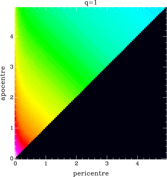
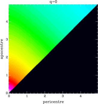
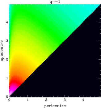
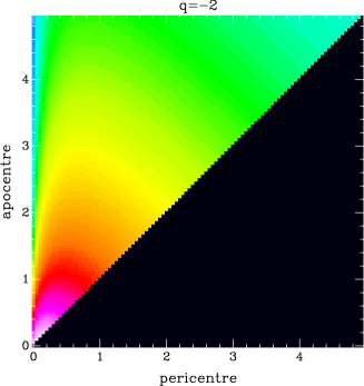
Figure 1: Turning-point diagram for several Hernquist models of the first family of §3.2. The colour shows how the density of orbits varies with pericentre and apocentre. Density declines from a high of white at the very centre, and then through the spectrum from red to a low of blue. Note the high red densities of elongated orbits along the left boundary for the most radial $q=1$ model, and their steady decline with increasing tangentiality as $q$ decreases.

We define $F_{q}^{p}(E,L)$ to be the component of the distribution function which corresponds to the component $r^{-q}(1+r)^{q}\psi^{p}$ of augmented density. It is given by formulas (77) and (79) in Appendix B. The full distribution function is then found by summing

$${\cal F}(E,L,\gamma,q)=\frac{3-\gamma}{4\pi}\sum_{p=4}^{\infty}C(\gamma,p,q)F_{q}^{p}(E,L),$$ (15)

where the coefficients $C(\gamma,p,q)$ are defined as

$$C(\gamma,p,q)=(-1)^{p}(2-\gamma)^{p}\sum_{k=0}^{4}(-1)^{k}{4\choose k}{\frac{k+q-\gamma}{2-\gamma}\choose p}.$$ (16)

The distribution function components $F_{q}^{p}(E,L)$ do not depend on the parameter $\gamma$. This parameter influences the rapidity with which the series (15) converges through the coefficients $C(\gamma,p,q)$, and especially their dependence on the power $(2-\gamma)^{p}$. Hence the closer $\gamma$ is to 2, the more rapidly does the series (15) converge.

The elementary distribution functions are simpler in certain special cases which are featured in the figures. For $q\in[1,0,-1,-2]$, we have

$$F_{q}^{p}(E,L)=\frac{pE^{p}}{(2\pi E)^{3/2}}\left[\frac{\Gamma(p)}{\Gamma(p-\frac{1}{2})}+\frac{q\sqrt{2E}}{\sqrt{\pi}L}\right. \times \left.\left\{\begin{array}[]{lll}1,&&q=0,1,\\ \ _{2}F_{1}\left(\frac{1}{2},-q;p,-\frac{2E}{L^{2}}\right),&&q=-1,-2.\end{array}\right\}\right].$$ (19)

As we see from equation (26) below, $q/2$ gives the central value of Binney’s anisotropy parameter, and hence An & Evans’s (2006b) cusp slope-central anisotropy theorem restricts $q$ to the range $q\leq\gamma$. It is also necessary that $q<2$ because ${\cal F}$ grows as $L^{-q}$ as $L\to 0$ when $q>0$ (See equation (79)), and the integration over ${\cal F}$ in equation (5) diverges if $q\geq 2$.

The expansion of the augmented density in powers of $\psi$ is simple for the $\gamma=1$ Hernquist models, for which

$$C(1,p,q)=(-1)^{p}{q-1\choose p-4},\qquad p\geq 4.$$ (20)

We display distribution functions for these models for different $q$ values in Fig. 1. They are plotted there in peri- and apocentre space. Circular orbits lie along the lower diagonal boundary, while orbits become increasingly radial as the left vertical boundary is approached. Hence densities are larger near there for the radially anisotropic $q=1$ case relative to the isotropic $q=0$ case, but relatively smaller for the tangentially anisotropic $q=-1$ and $q=-2$ cases.

3.2.1 Explicit $q=1$ distribution functions for $\gamma\geq 1$

Equations (15) and (19) show that the distribution functions for $q=1$ have the simple form

$${\cal F}(E,L,\gamma,q=1)=f_{0}(E)+\frac{f_{1}(E)}{L}.$$ (21)

The two terms correspond to the two components $\rho_{0}(\psi)$ and $\rho_{1}(\psi)/r$ of the augmented density (14). That allows us to avoid the expansion in powers of $\psi$, and to calculate the two components directly combining the methods of Baes et al. (2005) and An & Evans (2006a) respectively as in Sections 2.2 and 3.1. The results, which are similar to but not the same as the earlier (11) and (12), are

$$f_{0}(E) = \frac{3-\gamma}{8\pi^{3}}\sqrt{2E}\left[-3(\gamma-5)\ _{2}F_{1}\left(1,\frac{-1-\gamma}{2-\gamma};\frac{3}{2};(2-\gamma)E\right)+8(\gamma-4)\ _{2}F_{1}\left(1,\frac{-\gamma}{2-\gamma};\frac{3}{2};(2-\gamma)E\right)\right.$$ (22)

$$\left.-6(\gamma-3)\ _{2}F_{1}\left(1,\frac{1-\gamma}{2-\gamma};\frac{3}{2};(2-\gamma)E\right)+(\gamma-1)\ _{2}F_{1}\left(1,\frac{3-\gamma}{2-\gamma};\frac{3}{2};(2-\gamma)E\right)\right],$$

and

$$f_{1}(E)=\frac{3-\gamma}{8\pi^{3}}\left\{1-\left[1-(2-\gamma)E\right]^{\frac{1}{2-\gamma}}\right\}^{3}\left\{5-\gamma+\frac{\gamma-1}{\left[1-(2-\gamma)E\right]^{\frac{1}{2-\gamma}}}\right\}.$$ (23)

This solution is also restricted to $\gamma\geq 1$, like that of Section 3.1, because otherwise ${\cal F}$ becomes negative in the physical range. However $\gamma$ may exceed $2$, because the limitation imposed by the series expansion in $\psi$ used to obtain the solutions in Section 3.2 no longer applies. The distribution functions are particularly simple for the $\gamma=1$ Hernquist case for which

$${\cal F}(E,L,1,1)=\frac{8E^{2}\sqrt{2E}}{5\pi^{3}}+\frac{E^{3}}{\pi^{3}L}.$$ (24)

3.3 Second-order moments

An analytical expression for the velocity dispersions of all models can be derived by means of equations (6) and (7). Since the augmented density is separable in $r$ and $\psi$ and depends on $r$ as $(1+r)^{q}r^{-q}$, the tangential velocity dispersion can easily be derived from equation (7) as

$$\sigma_{\theta}^{2}(r,q)=\left(1-\frac{q}{2}\frac{1}{1+r}\right)\sigma_{r}^{2}(r,q).$$ (25)

Hence Binney’s anisotropy parameter is the monotonic function

$$\beta(r)=1-\frac{\sigma_{\theta}^{2}(r)}{\sigma_{r}^{2}(r)}=\frac{q}{2(1+r)},$$ (26)

for all $\gamma$. It has the same sign as $q$. Systems are more radial than isotropic when $q>0$, and more tangential than isotropic when $q<0$ as seen in Fig. 3, though they all tend to isotropy at large $r$ where $\beta\to 0$. The condition $\sigma_{\theta}^{2}(r,q)\geq 0$ restricts $q\leq 2$. There is no lower limit on $q$, and the limit $q\to-\infty$ gives a system with all orbits circular.

The simple separable form of the augmented density in equation (14), combined with equation (6), leads to a compact explicit expression for the radial velocity dispersion for all $\gamma$ and $q$ in terms of an incomplete Beta function (Abramowitz & Stegun, 1965) as

$$\sigma_{r}^{2}(r,q)=r^{\gamma-q}(1+r)^{4+q-\gamma}B_{\frac{1}{1+r}}(5,2-2\gamma+q),$$ (27)

cf (Baes & Dejonghe, 2002). Fig. 2 shows the radial dispersion $\sigma_{r}(r,q)$ tending to a common form at large $r$ where all models tend to isotropy. Equation (27) shows that common form to be $1/\sqrt{5r}$. The figures also show that $\sigma_{r}(r,q)$ increases with increasing $q$ near the centre as the orbits there become more strongly radial.

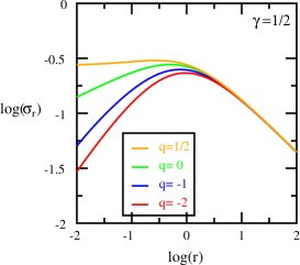
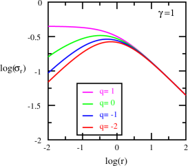
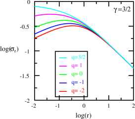
Figure 2: Radial velocity dispersion profiles for models of the first family for three $\gamma$ values. Dispersions increase with $q$, and the top curve corresponds to the highest allowed value $q=\gamma$.

Figure 3: The variation of the anisotropy parameter with radius $r$ for the models of §3.2. It is independent of the model parameter $\gamma$.

3.4 Energy distribution

The anisotropic models differ in way in which energy is distributed among their orbits. We label the part of the mass density that is contributed by the energy range $[E,E+dE]$ as the energy density ${\cal F}_{E}$. It is given by the inner integral of equation (5) as

$${\cal F}_{E}(\psi,r,E)=2\pi\int_{0}^{2(\psi-E)}\frac{{\cal F}(E,L)}{\sqrt{2(\psi-E)-v_{t}^{2}}}dv_{t}^{2}.$$ (28)

We define as $F_{E,q}^{p}(\psi,r,E)$ the components of energy density which are obtained with the elementary distribution functions $F_{q}^{p}(E,L)$ on the right hand side of this equation (28). They are evaluated in Appendix A. Then the energy density for the full model is given by the sum

$${\cal F}_{E}(\psi,r,E)=\frac{3-\gamma}{4\pi}\sum_{p=4}^{\infty}C(\gamma,p,q)F_{E,q}^{p}(\psi,r,E),$$ (29)

with the coefficients $C(\gamma,p,q)$ that were introduced in equation (16). The energy density for the simple $\gamma=q=1$ distribution function (24) is

$${\cal F}_{E}(\psi,r,E)=\psi^{3}\left[\frac{64}{5\pi^{2}}\left(\frac{E}{\psi}\right)^{5/2}\sqrt{1-\frac{E}{\psi}}+\frac{2}{\pi r}\left(\frac{E}{\psi}\right)^{3}\right],\quad 0\leq\frac{E}{\psi}\leq 1.$$ (30)

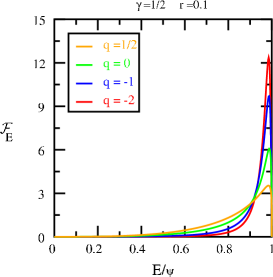
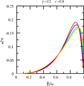
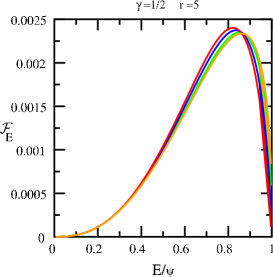
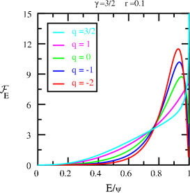
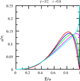
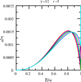
Figure 4: Energy densities for the $\gamma=1/2$ and $\gamma=3/2$ models of the first family at spatial radii $r=0.1$, $r=0.8$, and $r=5$. The same colour-codings of the values of $q$ are used through each row. The energy $E$ is scaled with its maximum value $\psi(r)$ at that radius. Each curve in a panel encloses the same area. That area is the local mass density divided by $\psi$, and varies from panel to panel with both $r$ and $\gamma$. The singular growth of the $q=\gamma=3/2$ curve for $r=5$ does not occur until $E/\psi>0.999$.

Fig. 4 shows the energy densities for two values of $\gamma$ at three radii: one small, one intermediate, and one large. We chose the $\gamma$ values of $1/2$ and $3/2$ to represent the range $0<\gamma<2$ for which our solutions apply. ${\cal F}_{E}$ is more concentrated at higher energy at small $r$ for the more tangential models (smaller $q$) and less concentrated for the more radial models (larger $q$). The situation is reversed at large $r$. The reason is that the more radial orbits are less tightly bound than the more tangential ones near the center, while the opposite is the case at large $r$. Fig.1 of Dejonghe (1987) for anisotropic Plummer models shows the same phenomenon, though our ${\cal F}_{E}$ are more concentrated towards high energies than his because our $\gamma$-models are more centrally concentrated than his Plummer model. Also, unlike his, the differences between our models diminish at large $r$ where they become isotropic.

Whereas ${\cal F}_{E}$ drops to zero at the upper limit $E/\psi=1$ for all of the upper row of $\gamma=1/2$ models, and also for the $q\leq 1$, $\gamma=3/2$ models of the lower row, it becomes infinite as $E/\psi\to 1$ for the most radial and most cuspy $q=\gamma=3/2$ model, and has a finite limit for the $q=1$ model, as in the $\gamma=1$ case in equation (30). This behaviour is a consequence of the $(1-E/\psi)^{(1-q)/2}$ dependence of $F^{p}_{E,q}$ for $E/\psi>r^{2}/(1+r^{2})$ given by equation (83). That dependence is a consequence of the $L^{-q}$ dependence of the distribution function for $L^{2}<2E$ as given by equation (79).

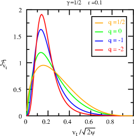
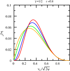
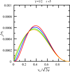
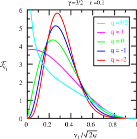
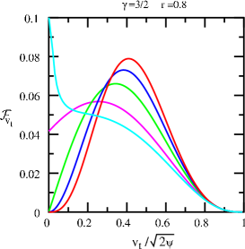
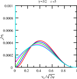
Figure 5: The transverse velocity densities for the $\gamma=1/2$ and $\gamma=3/2$ models of the first family at spatial radii $r=0.1$, $r=0.8$, and $r=5$. The same colour-codings of the values of $q$ are used through each row. The transverse velocity is scaled with its maximum value $\sqrt{2\psi}$ at that radius. All the curves in a single panel again enclose the same area; it is now the local mass density divided by $\sqrt{2\psi}$.

3.5 Distribution of the transverse motions

The anisotropic models also differ in way in which transverse velocity is distributed among their orbits. We label the part of the mass density which is contributed by the transverse velocity range $[v_{t},v_{t}+dv_{t}]$ as the transverse velocity density ${\cal F}_{v_{t}}$. It is given by the inner integral of equation (5), after the order of its integrations has been changed, as

$${\cal F}_{v_{t}}(\psi,r,v_{t})=4\pi v_{t}\int_{0}^{\psi-v_{t}^{2}/2}\frac{{\cal F}(E,L)}{\sqrt{2(\psi-E)-v_{t}^{2}}}dE.$$ (31)

We evaluate the transverse velocity densities $F_{v_{t},q}^{p}(\psi,r,v_{t})$ corresponding to the elementary distribution functions $F_{q}^{p}(E,L)$ in Appendix A. The transverse velocity density for the full model is

$${\cal F}_{v_{t}}(\psi,r,v_{t})=\frac{3-\gamma}{4\pi}\sum_{p=4}^{\infty}C(\gamma,p,q)F_{v_{t},q}^{p}(\psi,r,v_{t}),$$ (32)

with the same coefficients $C(\gamma,p,q)$ as before. The transverse velocity density for the simple $\gamma=q=1$ distribution function (24) is

$${\cal F}_{v_{t}}(\psi,r,v_{t})=\frac{(2\psi)^{7/2}}{4\pi}\left[t(1-t^{2})^{3}+\frac{32}{35\pi r}(1-t^{2})^{7/2}\right],\quad 0\leq t=\frac{v_{t}}{\sqrt{2\psi}}\leq 1.$$ (33)

Fig. 5 shows the transverse velocity densities for the same set of models as those whose energy densities were shown in Fig. 4. Now ${\cal F}_{v_{t}}$ is generally more concentrated toward low velocities at small $r$ for the more tangential models (smaller $q$) and less so for the more radial models (larger $q$). The situation is reversed at large $r$, though differences there are small because our models tend to isotropy there. Fig. 4 of Dejonghe (1987) for anisotropic Plummer models shows similar behaviour at small radii. The generally higher transverse velocities at small $r$ for the more radial models is due to orbits which are close to their turning points and so have transverse velocities which are well in excess of the local circular velocity.

The $L^{-q}$ dependence of the distribution function for $L^{2}<2E$ again has an important effect. It is now seen as $v_{t}\to 0$. Equation (87) shows that $F^{p}_{v_{t},q}$ varies as $v_{t}^{1-q}$ for $v_{t}/\sqrt{2\psi}<1/\sqrt{1+r^{2}}$. It tends to $0$ as $v_{t}\to 0$ for $q<1$, has a finite limit there for $q=1$, and becomes infinite for $q>1$. The infinite growth is more prominent for the $\gamma=3/2$ models of Fig. 5 than for those of Fig. 4 because of its lower power (-1/2 rather than -1/4).

3.6 Observable properties

Figure 6: The projected density distribution for different $\gamma$-models.

The projected density of a $\gamma$-model is found from the relation

$$\Sigma(R)=2\int_{R}^{\infty}\frac{r\rho(r)dr}{\sqrt{r^{2}-R^{2}}},$$ (34)

where we align the $z$-axis with the line-of-sight, and $R=\sqrt{x^{2}+y^{2}}$ is the usual plane polar coordinate, now in the plane of the sky. The projected velocity dispersion $\sigma_{p}(R)$ is given by (Binney & Mamon, 1982; Binney & Tremaine, 1987)

$$\sigma_{p}^{2}(R)=\frac{2}{\Sigma(R)}\int_{R}^{\infty}\left[1-\frac{R^{2}}{r^{2}}\beta(r)\right]\frac{r\rho(r)\sigma_{r}^{2}(r)dr}{\sqrt{r^{2}-R^{2}}}.$$ (35)

The integrations needed for both (34) and (35) must be done numerically for $\gamma$-models. Projected densities of some $\gamma$-models are shown in Fig. 6; the dependence of the central density slope on the parameter $\gamma$ is clearly visible in projection. Projected velocity dispersions are shown in Fig. 7. They decrease monotonically with the projected radius $R$ in radial systems, but can have a central peak for tangential systems when the tangential component of the velocity dispersion becomes increasingly important with increasing $R$.

The normalised line-of-sight velocity profile $l(v_{z},R)$ describes the distribution of $v_{z}$ along the line-of-sight. It is obtained by integrating the distribution function over the velocities $v_{R}$ and $v_{\varphi}$ in the plane of the sky, followed by a spatial integration along the line-of-sight. It is given by

$$\Sigma(R)l(v_{z},R)=2\int_{R}^{\infty}\frac{rdr}{\sqrt{r^{2}-R^{2}}}\int\!\!\!\int_{0\leq v_{R}^{2}+v^{2}_{\varphi}\leq 2\psi-v_{z}^{2}}dv_{R}dv_{\varphi}{\cal F}(E,L).$$ (36)

It falls to zero at the extremities $v_{z}=\pm\sqrt{2\psi(R)}$. We express the arguments of the distribution function ${\cal F}$ as

$$E=\psi-\frac{1}{2}(v_{z}^{2}+v_{R}^{2}+v^{2}_{\varphi}),\quad L=\sqrt{r^{2}v^{2}_{\varphi}+(zv_{R}-Rv_{z})^{2}},$$ (37)

and integrate using polar coordinates in $(v_{R},v_{\varphi})$ velocity space. The area under the normalised velocity profile is unity because integrating ${\cal F}$ over all three velocity component $v_{z}$ gives the density $\rho(r)$. Hence integrating the right hand side of equation (36) over $v_{z}$ gives the projected density $\Sigma$, and hence integrating both sides of equation (36) over $v_{z}$ leads to the result $\int l(v_{z},R)dv_{z}=1$.

Fig. 8 shows normalised line-of-sight velocity profiles for models of the first family for three values of $\gamma$, all obtained by evaluating equation (36) numerically. The most striking feature of these profiles is how much more they vary at small radii with the central density slope $\gamma$ than with the orbital composition. The profiles of the more tangential models are a little narrower at small radii for all $\gamma$, and slightly broader at large radii where they are almost isotropic. Other features that stand out are the discontinuous slopes at $v_{z}=0$ of $q=1$ profiles, and the sharp cusps there of $q=1.5$ profiles. They are further visible effects of the $L^{-q}$ dependence of the distribution functions for $L^{2}<2E$.

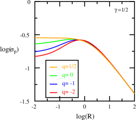
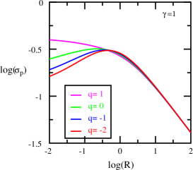
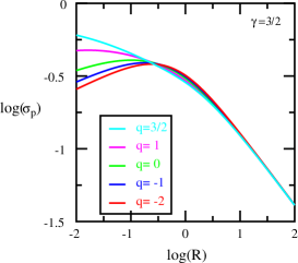
Figure 7: The projected velocity dispersion profiles for the same set of models as in Fig. 2.

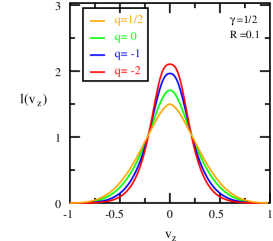
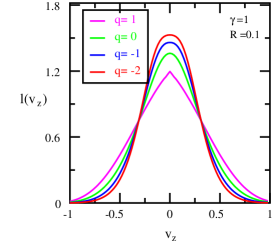
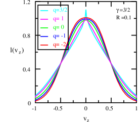
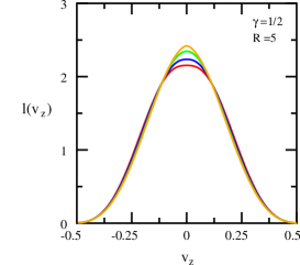
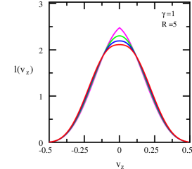
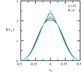
Figure 8: The normalised line-of-sight velocity profiles at projected radii $R=0.1$ and $R=5$ for models with three different values of $\gamma$. The same colour-codings are used in each column, i.e. for each $\gamma$.

4 More anisotropic models

The models introduced in Section 3.2 are all isotropic at large radii. If isotropy is a consequence of mixing, then it is more likely that galaxies are isotropic in their well-mixed centres than in their outer regions. We now construct a second family of models which are isotropic at their centres but anisotropic at larger radii. We do this by modifying the method of the previous section, in a way which allows us to use similar mathematics. We derive the distribution functions of these models in §4.1. We give their velocity dispersions, energy and transverse velocity distributions, and projected line profiles in the next two sections. Then in a brief final section §4.4, we construct some extreme $\gamma$-models for which all orbits are radial.

4.1 Another two-parameter family of anisotropic models

We obtain these by writing the augmented density in the form of $(1+r)^{q}$ times a function of $\psi$ as

$$\rho(\psi,r)=\frac{3-\gamma}{4\pi}(1+r)^{q}[1-(2-\gamma)\psi]^{\frac{-\gamma}{2-\gamma}}\left\{1-[1-(2-\gamma)\psi]^{\frac{1}{2-\gamma}}\right\}^{4+q}.$$ (38)

As a result, Binney’s anisotropy parameter is now

$$\beta(r)=-\frac{qr}{2(1+r)},$$ (39)

and has the opposite sign to $q$. It is zero at the isotropic centre, and tends to $-q/2$ at large distances (see Fig. 9). Systems are more strongly radial in the outer regions for negative $q$, and more tangential for positive $q$. The parameter $q$ is restricted to $q\geq-2$ by the requirement that $\sigma_{\theta}^{2}\geq 0$, but it is no longer restricted by An & Evans’s (2006b) cusp slope-central anisotropy theorem because the centre is isotropic. Models with the extreme value $q=-2$ are purely radial at large distances.

The augmented density (38) varies as $\psi^{4+q}$ for small $\psi$. Hence its expansion in powers of $\psi$ now ascends in integer steps from that initial term, and has the form

$$\rho(\psi,r)=\frac{3-\gamma}{4\pi}(1+r)^{q}\sum_{j=0}^{\infty}{\bar{C}}(\gamma,4+q+j,q)\psi^{4+q+j},$$ (40)

for suitable coefficients ${\bar{C}}$. The distribution function is

$${\cal F}(E,L,\gamma,q)=\frac{3-\gamma}{4\pi}\sum_{j=0}^{\infty}{\bar{C}}(\gamma,4+q+j,q){\bar{F}}_{q}^{4+q+j}(E,L).$$ (41)

where ${\bar{F}}_{q}^{p}(E,L)$ is defined to be the component of the distribution function which corresponds to the component $(1+r)^{q}\psi^{p}$ of augmented density. Formulas for it, which again do not depend on the parameter $\gamma$, are given in Appendix B.

Figure 9: The anisotropy parameter $\beta$ as a function of radius $r$ for the second family of models of §4.1. It is again independent of the model parameter $\gamma$.

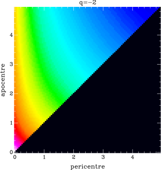
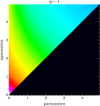
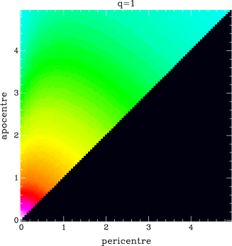
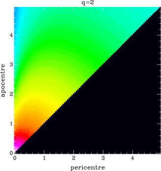
Figure 10: Turning-point diagrams, coded as in Fig. 1, but now for Hernquist models of the second family. The predominance of near-radial orbits in the $q=-2$ model, and their decline as $q$ increases can be seen clearly seen. There is no $q=0$ plot because it is the same as that in Fig. 1

The evaluation of the coefficients ${\bar{C}}$ is now more complicated. The method of the previous section in which we expand first in powers of $[1-(2-\gamma)\psi]$ and then in powers of $\psi$, yields an expansion in integer powers of $\psi$, and so is valid only when $(q+4)$ is a positive integer. For those cases

$${\bar{C}}(\gamma,4+q+j,q)=(-1)^{p}(2-\gamma)^{p}\sum_{k=0}^{4+q}(-1)^{k}{4+q\choose k}{\frac{k-\gamma}{2-\gamma}\choose 4+q+j}.$$ (42)

As before, the closer $\gamma$ is to 2, the more rapidly does the series (41) converge.

More generally, one must expand the augmented density (38) directly in powers of $\psi$ without any intermediate expansion. That leads to an infinite series in $\psi$ for $1-[1-(2-\gamma)\psi]^{1/(2-\gamma)}$ and the need to multiply the $(4+q)$th power of that infinite series with another infinite series. This procedure does simplify when $1/(2-\gamma)$ is a positive integer. The simplest instances are the $\gamma=1$ Hernquist and the $\gamma=\frac{3}{2}$ Dehnen models for which

$${\bar{C}}(1,4+q+j,q)=1,\qquad{\bar{C}}\left(\frac{3}{2},4+q+j,q\right)=\frac{1}{2^{j+1}}\sum_{k=0}^{j}\left(-\frac{1}{2}\right)^{k}(j-k+1)(j-k+2){4+q\choose k}.$$ (43)

Although the infinite series expansions (41) are limited to the range $0<\gamma<2$ by the same convergence conditions as in §3.2, that limitation disappears when the sum in (40) is finite. It is finite for the most radial $q=-2$ case when $1/(\gamma-2)$ is a positive integer, as for $\gamma=5/2$. Equation (41) then gives exact distribution functions for strongly radial models with steep cusps.

The elementary distribution functions are again simpler for some small integer values of $q$. Specifically, equation (80) gives

$${\bar{F}}^{p}_{q}={\Gamma(p+1)E^{p}\over(2\pi E)^{3/2}}\left\{{1\over\Gamma(p-{1\over 2})}+{2q\over\sqrt{\pi}\Gamma(p-1)}{L\over\sqrt{2E}}+{q(q-1)\over 2\Gamma(p-{3\over 2})}{L^{2}\over 2E}\right\},$$ (44)

for $q=0,1,2$, and equation (78) gives

$${\bar{F}}^{p}_{q}={E^{p}\over\sqrt{\pi}(2\pi E)^{3/2}}\left({\sqrt{2E}\over L}\right)^{-2q-1}{\Gamma(p+1)\over\Gamma(p-1-q)}{}_{2}F_{1}\left(-q-{1\over 2},-q;p-q-1;-{2E\over L^{2}}\right),$$ (45)

for $q=-1,-2$. Exact distribution functions of the forms ${\cal F}(E,L,\gamma,q=1)=f_{0}(E)+Lf_{1}(E)$ and ${\cal F}(E,L,\gamma,q=2)=f_{0}(E)+Lf_{1}(E)+L^{2}f_{2}(E)$ for $q=1$ and $q=2$ respectively can be found by the methods of An & Evans (2006a). The results, which are similar to those of §3.2.1, are given in Appendix B.4.

4.1.1 Explicit distribution functions for Hernquist models

The fact that each ${\bar{C}}$ coefficient is 1 for Hernquist models allows the summations needed for the full distribution function (41) to be performed explicitly for the simple ${\bar{F}}^{p}_{q}$ functions listed above. Those for $q=-1$ and $q=-2$ can be done using Euler’s formula (15.3.1) of Abramowitz & Stegun (1965) for hypergeometric functions which gives

$${}_{2}F_{1}\left(-q-{1\over 2},-q;p-q-1;-{2E\over L^{2}}\right)=\frac{\Gamma(p-1-q)}{\Gamma(-q)\Gamma(p-1)}\int_{0}^{1}t^{-q-1}(1-t)^{p-2}\left(1+\frac{2Et}{L^{2}}\right)^{q+\frac{1}{2}}dt.$$ (46)

This integral converges for all positive $E$, regardless of the magnitude of $L^{2}$. Using it, the series summation $\sum_{j=0}^{\infty}(j+2)(j+1)x^{j}=2/(1-x)^{3}$ and a change of integration variable to $y=Et$, we obtain the compact integrals

$${\cal F}(E,L,\gamma=1,q) = \left\{\begin{array}[]{lll}\frac{1}{2\pi^{3}}\int_{0}^{E}\frac{dy}{(L^{2}+2y)^{1/2}}\left[\frac{1}{(1-E+y)^{3}}-1\right],&&q=-1,\\ \frac{1}{\pi^{3}}\int_{0}^{E}\frac{ydy}{(L^{2}+2y)^{3/2}(1-E+y)^{3}},&&q=-2,\end{array}\right.$$ (49)

for the two distribution functions. They are evidently non-negative everywhere, and so physically acceptable. The integrals (49) can be evaluated by elementary methods as

$${\cal F}(E,L,1,-1)=\frac{1}{2\pi^{3}}\left\{\frac{3}{2\chi^{2}}\left[I_{1}+\sqrt{L^{2}+2E}-\frac{L}{(1-E)}\right]+\frac{1}{2\chi}\left[\sqrt{L^{2}+2E}-\frac{L}{(1-E)^{2}}\right]-\sqrt{L^{2}+2E}+L\right\},$$ (50)

and

$${\cal F}(E,L,1,-2)=\frac{2(1-E+2L^{2}){\cal F}(E,L,1,-1)}{\pi}+\frac{1}{\pi^{3}\chi}\left[\frac{L^{2}}{\sqrt{L^{2}+2E}}-\frac{L}{(1-E)^{2}}+(1-E+2L^{2})(\sqrt{L^{2}+2E}-L)\right],$$ (51)

where

$$\chi=2(1-E)-L^{2},\qquad I_{1}=\int_{0}^{E}\frac{dy}{(L^{2}+2y)^{1/2}(1-E+y)} = \left\{\begin{array}[]{lll}\frac{2}{\sqrt{\chi}}\left[\arctan\frac{\sqrt{L^{2}+2E}}{\sqrt{\chi}}-\arctan\frac{L}{\sqrt{\chi}}\right],&&\chi>0,\\ \frac{1}{\sqrt{-\chi}}\ln\left[\frac{(\sqrt{L^{2}+2E}-\sqrt{-\chi})(L+\sqrt{-\chi})}{(\sqrt{L^{2}+2E}+\sqrt{-\chi})(L-\sqrt{-\chi})}\right],&&\chi<0.\end{array}\right.$$ (54)

Both distribution functions vary smoothly across the curve $2(1-E)=L^{2}$ where

$${\cal F}(E,\sqrt{2(1-E)},1,-1) = \frac{1}{\pi^{3}\sqrt{2}}\left\{\frac{1}{5}\left[\frac{1}{(1-E)^{5/2}}-1\right]+\sqrt{1-E}-1\right\},$$ (55)

$${\cal F}(E,\sqrt{2(1-E)},1,-2) = \frac{1}{\pi^{3}\sqrt{2}}\left\{\frac{1}{5}\left[\frac{1}{(1-E)^{5/2}}-1\right]+\frac{(1-E)}{7}\left[1-\frac{1}{(1-E)^{7/2}}\right]\right\}.$$ (56)

We display distribution functions for these models for different $q$ values in Fig.10. They now show increasing radiality with decreasing $q$, and can be compared with those of Fig.1. The $q=0$ case, missing from Fig.10, is the same as that shown in Fig.1.

Figure 11: The radial velocity dispersion profiles for three $\gamma$ values for the second family, and for $q=-2,-1,0,1,2$. The highest curve is for the lowest value of $q$ and the others follow in sequence.

4.2 Second-order moments

The velocity dispersions are now related by

$$\sigma_{t}^{2}(r,q)=\left[1+\frac{qr}{2(1+r)}\right]\sigma_{r}^{2}(r,q).$$ (57)

and the radial velocity dispersions are

$$\sigma_{r}^{2}(r,q)=r^{\gamma}(1+r)^{4+q-\gamma}B_{1/(1+r)}(5+q,2-2\gamma).$$ (58)

Equation (58), when approximated for large $r$, shows that the radial velocity dispersion $\sigma_{r}(r,q)\approx 1/\sqrt{(5+q)r}$ for large $r$ and increases as $q$ becomes more negative. The radial velocity dispersion near the centre behaves differently according to whether $\gamma$ is greater or less than $1$. It has the form $\sigma_{r}(r,q)\approx\sqrt{r^{2-\gamma}/[2(\gamma-1)]}$, and $\sigma_{r}(r,q)\approx\sqrt{(-r\ln r)}$ in the limit $\gamma=1$, which is independent of $q$ when $\gamma\geq 1$. It depends on $q$ for weaker cusps with $\gamma<1$. Then $\sigma_{r}(r,q)\approx\sqrt{r^{\gamma}B(5+q,2-2\gamma)}$, and is larger for the more radial models even near the centre as Fig. 11 confirms.

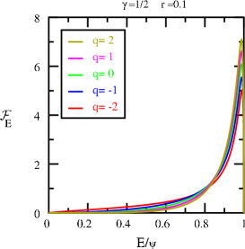
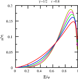
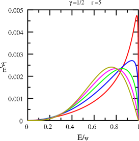
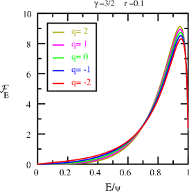
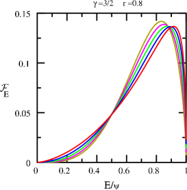
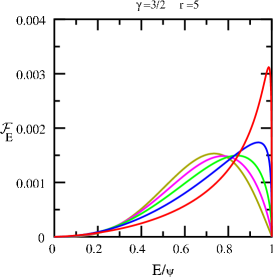
Figure 12: Energy densities, as in Fig. 4, but for now for models of the second family.

4.3 Other properties

We define energy and transverse velocity densities ${\bar{F}}_{E,q}^{p}(\psi,r,E)$ and ${\bar{F}}_{v_{t},q}^{p}(\psi,r,v_{t})$ corresponding to elementary distribution functions ${\bar{F}}_{q}^{p}(E,L)$ in the same way as we defined $F_{E,q}^{p}(\psi,r,E)$ and $F_{v_{t},q}^{p}(\psi,r,v_{t})$ in §3.4 and 3.5. The energy and transverse velocity densities are then given by sums of the same form as those of equation (29) and (32) but now with barred components.

Energy densities for models of the second family shown in Fig. 12 show the same relative differences between more tangential (now larger $q$) and more radial (smaller $q$) as do the models of the first family shown in Fig. 4. The differences are now small at small $r$ because models of the second family are isotropic at their centres. Differences appear as the radius increases. The most radial $q=-2$ model remains strongly peaked even at high $E/\psi$, while the peaks of the other models move to lower relative energies with increasing radius and decreasing radiality, as in Dejonghe’s Fig. 1. All ${\cal F}_{E}$ curves now drop to zero at the right limit $E/\psi=1$ because the distribution functions are not singular as $L\to 0$. Our ${\cal F}_{E}$ are again more concentrated towards high energies than those of Dejonghe (1987) because our densities are more centrally concentrated than his.

The transverse velocity densities in Fig.13 are also similar at small radii. This distribution remains strongly peaked at low relative $v_{t}$ for the most radial $q=-2$ model at large radii, while the peaks of the other distributions become increasingly central with increasing radius and increasing tangentiality. Dejonghe’s Fig. 4 shows similar behaviour at large radii.

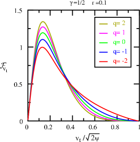
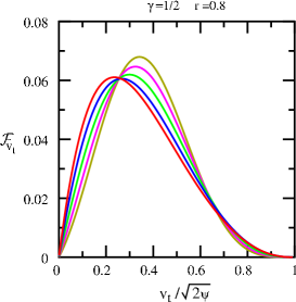
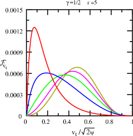
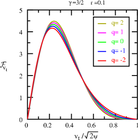
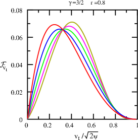
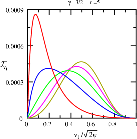
Figure 13: The transverse velocity densities, as in Fig. 5, but for now for models of the second family.

Projected velocity dispersions for the second family are shown in Fig. 14. All now peak at an intermediate projected radius $R$. Unlike the unprojected radial velocity dispersions shown in Fig. 11, the projected ones become larger near the centre and smaller in the outer regions as the radiality increases.

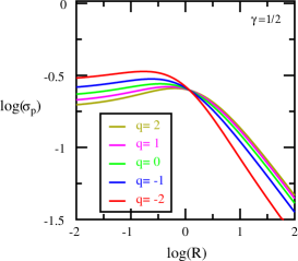
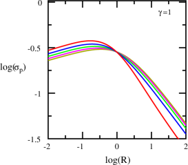
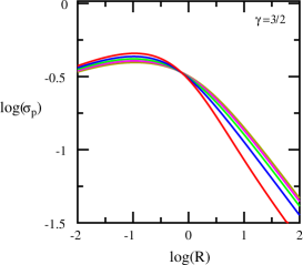
Figure 14: The projected velocity dispersion profiles for the same models as in Fig. 11.

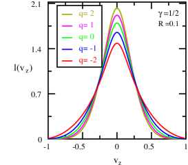
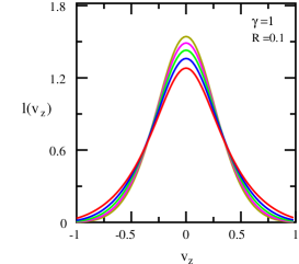
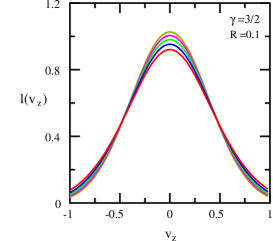
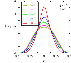
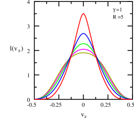
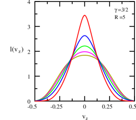
Figure 15: The normalised line-of-sight velocity profiles for models of the second family for the same $R$ and $\gamma$ values as Fig. 8.

Fig. 15 shows normalised line-of-sight velocity profiles for models of the second family for three values of $\gamma$ and at the same radii as those of Fig. 8. They too vary more at small radii with the central density slope $\gamma$ than with the orbital composition. The profiles of the more tangential models are now more noticeably narrower at small radii and broader at large radii than the models of the first family. Now that the distribution functions are isotropic at their centres, their velocity profiles peak smoothly at $v_{z}=0$.

4.4 Models with all radial orbits

Models with all radial orbits have distribution functions of the form

$${\cal F}(E,L,\gamma)=f(E)\delta(L^{2}).$$ (59)

With this form, equation (5) becomes the following Abel integral equation for $f(E)$ (Richstone & Tremaine, 1984):

$$r^{2}\rho=2\pi\int_{0}^{\psi}\frac{f(E)dE}{\sqrt{2(\psi-E)}}.$$ (60)

Physical solutions are possible only if $\lim_{r\to 0}r^{2}\rho>0$, because (60) gives $r^{2}\rho$ as a weighted integral of $f(E)$ over the whole physical range of $E$, and so a zero value would imply that there are unphysical negative values of $f(E)$ (Richstone & Tremaine, 1984). The solution of equation (60) is obtained using the same $t$-substitution as in Baes et al. (2005) §5.2. It is positive everywhere, and hence always physical, because it is an integral with a positive integrand. It can be expressed in hypergeometric functions as

$$f(E)=\frac{3-\gamma}{4\pi^{3}}\sqrt{2E}\left[\gamma-2-2(\gamma-3)\ _{2}F_{1}\left(1,\frac{1}{\gamma-2};\frac{3}{2};(2-\gamma)E\right)+(\gamma-4)\ _{2}F_{1}\left(1,\frac{2}{\gamma-2};\frac{3}{2};(2-\gamma)E\right)\right].$$ (61)

This expression provides analytical $\gamma$-models for the range $2\leq\gamma<3$, and adds to the only previously-known analytical model with all radial orbits (Fridman & Polyachenko 1984, Binney & Tremaine 1987, problem 4-19). The hypergeometric functions are elementary for the strong cusp case of $\gamma=\frac{5}{2}$, as they are for that case in Tremaine et al. (1994), and give

$${\cal F}(E,L,\frac{5}{2})=\frac{\sqrt{2E}\delta(L^{2})}{8\pi^{3}}\left\{\frac{1}{2}\right. + \left.\frac{1}{2(2+E)}-\frac{5}{4(2+E)^{2}}-\frac{15}{4(2+E)^{3}}\right.$$ (62)

$$+ \left.\frac{2\ln\left[\sqrt{1+\frac{E}{2}}+\sqrt{\frac{E}{2}}\right]}{\sqrt{E}(2+E)^{3/2}}\left[1-\frac{15}{4(2+E)^{2}}\right]\right\}.$$

5 Conclusions

We have provided a wide range of analytical anisotropic stellar dynamic distribution functions for the widely used $\gamma$ density profile. The simplest are two one-parameter families with constant anisotropy, those of §3.1 for $\gamma\geq 1$ for which Binney’s parameter $\beta=0.5$, and the all-radial models of §4.4 for $\gamma\geq 2$ for which $\beta=1$. Only the $\gamma=1$ member of the first family was known previously (Baes & Dejonghe, 2002).

The two two-parameter families of §3.2 and §4.1 provide a much wider range. They have a second parameter $q$ in addition to $\gamma$. It controls their anisotropy. The first family is isotropic at large distances, and $q$ gives the value of $2\beta$ at its centre. The second family is isotropic at its centre, and $q$ gives the value of $-2\beta$ at large distances. A greater variety of behaviour can be obtained by combining members of the families, as in Dejonghe (1989) and Baes & Dejonghe (2002), though we have not done this.

Finite expressions are given for some of the distribution functions. These include those in §3.2.1 for models of the first family with $q=1$, and in Appendix B.4 for tangentially biased models of the second family with $q=1$ and $q=2$. Other more restricted cases are the radially biased Hernquist models of the second family of §4.1.1 with $q=-1$ and $q=-2$ (most radial), and the strongly cusped $q=-2$, $\gamma=2+1/N$, $N$ an integer, cases identified, though not studied, in §4.1. More generally, distribution functions must be found by summing series of ordinary or generalised hypergeometric functions using formulas given in Appendix B. The coefficients of those series depend on powers of $(2-\gamma)$, and the series converge rapidly for $\gamma$ close to 2 when few terms are needed. Conversely, long series are needed to generate the $\gamma=0.5$ plots shown in the figures. It is not difficult to compute hypergeometric functions; some advice on how to do so is given at the end of Appendix A.

The first family of models, which are radially biased at their centres when $q>0$, provide an interesting example of the cusp slope-central anisotropy theorem of An & Evans (2006b). That theorem states that the central value of $\beta$ can not exceed half the density slope $\gamma$. In fact our models show that their theorem is somewhat more widely applicable than their discussion of it allows. Their proof assumes that the distribution function has a Laurent expansion of a specific form in the whole neighbourhood of $L=0$. Our equations (15) and (79) show that our distribution functions have this form but not in the whole neighbourhood of $L=0$, only in the region $L^{2}<2E$. A different form, given by equations (15) and (77) applies in $0<2E<L^{2}$, which includes a part of the neighbourhood of $L=0$ near $E=0$. Nevertheless their theorem is still valid, and their proof of it requires no essential change, because a Laurent expansion of the form they assume is valid near the cusp and its component that is proportional to $L^{-q}$ dominates the behaviour there. The wholly radial models of §4.4 with $\beta=1$ everywhere respect the singular $q\to 2$ limit of their theorem because they exist only for $\gamma\geq 2$.

Besides distribution functions, we have given and displayed velocity dispersions, energy and transverse velocity densities, and observable properties, including line-of-sight velocity profiles. The singular central behaviour of the radially biased models of the first family is evident in the $q\geq 1$ curves in Fig. 4, Fig. 5, and Fig. 8. The latter are particularly significant since they plot a directly observable quantity. The $\gamma$-models are commonly used to describe the kinematics at the cores of giant elliptical galaxies, both to model observations and to derive initial conditions for either N-body or Monte-Carlo simulations. Because of the past lack of analytical models, many workers have used Hernquist’s (1993) simplified procedure to generate approximate distribution functions. Kazantzidis, Magorrian & Moore (2004) have shown that this procedure can be hazardous when applied to galaxies that are strongly non-Gaussian, as it can then lead to an initial state that is far from equilibrium. We have identified cusped galaxies with $\beta\geq 0.5$ at their centres and whose line-of-sight velocities are cusped as instances of non-Gaussian behaviour. The wide variety of analytic distribution functions of this paper provides alternatives to the use of Hernquist’s method. Our distribution functions are in exact equilibrium. They can be coupled with a three-dimensional Monte-Carlo simulator to provide valid initial conditions for N-body and Monte-Carlo simulations (Buyle et al., 2006), and so avoid the subsequent development being influenced by artifacts of the start.

Appendix A Evaluation of distribution and related functions

We defined $F_{q}^{p}(E,L)$ in section 3.2 to be the distribution function which corresponds to the elementary augmented density $r^{-q}(1+r)^{q}\psi^{p}$. We find it by taking a Laplace-Mellin transform in $E$ and $L=rv_{t}$ as in (Dejonghe, 1986), and obtain

$$\mathcal{L}_{E\to\alpha}\mathcal{M}_{L\to\beta}\{{\cal F}(E,L)\}=\frac{2^{\beta/2}}{(2\pi)^{3/2}}\frac{\alpha^{(3-\beta)/2}}{\Gamma(1-\beta/2)}\mathcal{L}_{\psi\to\alpha}\mathcal{M}_{r\to\beta}\{\rho(\psi,r)\}=\frac{\Gamma(p+1)}{\alpha^{p+1}}\frac{\Gamma(\beta-q)\Gamma(-\beta)}{\Gamma(-q)}.$$ (63)

Although the Mellin transform of $r^{-q}(1+r)^{q}$ does not exist for non-integer $q>0$, the final distribution function which we obtain for $q<0$ is valid in a continous interval of $q$, and remains valid for $q>0$ by the principle of analytical combination; it suffices to check that the proper limits can be taken in Equation (79) in order to check the existence of our results. The Laplace transform with respect to $\alpha$ is easily inverted, and we are left with a Mellin inversion integral

$$F_{q}^{p}(E,L)=\frac{\Gamma(p+1)E^{p-3/2}}{(2\pi)^{5/2}2^{q}\Gamma(-q)}\frac{1}{2\pi i}\int_{\beta_{0}-i\infty}^{\beta_{0}+i\infty}\frac{\Gamma(-\frac{\beta}{2})\Gamma(\frac{1}{2}-\frac{\beta}{2})\Gamma(-\frac{q}{2}+\frac{\beta}{2})\Gamma(\frac{1}{2}-\frac{q}{2}+\frac{\beta}{2})}{\Gamma(1-\frac{\beta}{2})\Gamma(p-\frac{1}{2}+\frac{\beta}{2})}\left(\frac{L^{2}}{2E}\right)^{-\beta/2}d\left(\frac{\beta}{2}\right).$$ (64)

for $F_{q}^{p}(E,L)$. We have here used applied the duplication formula for the Gamma function (Abramowitz & Stegun, 1965) equation 6.1.18 to expand the product $\Gamma(\beta-q)\Gamma(-\beta)$. The inversion of the $\beta$-integral in equation (64) gives,

$$F_{q}^{p}(E,L)=\frac{\Gamma(p+1)E^{p-3/2}}{(2\pi)^{5/2}2^{q}\Gamma(-q)}G_{33}^{22}\left(\frac{L^{2}}{2E}\left|\begin{array}[]{ccccc}1&,&\frac{1}{2}&,&p-\frac{1}{2}\\ -\frac{q}{2}&,&\frac{1}{2}-\frac{q}{2}&,&0\end{array}\right.\right),$$ (65)

by matching to the definition 5.3.1 in Erdelyi (1953) of the Meijer G function $G^{22}_{33}$. A similar analysis for the elementary augmented density $(1+r)^{q}\psi^{p}$ gives

$${\bar{F}}_{q}^{p}(E,L)=\frac{\Gamma(p+1)E^{p-3/2}}{(2\pi)^{5/2}2^{q}\Gamma(-q)}G_{33}^{22}\left(\frac{L^{2}}{2E}\left|\begin{array}[]{ccccc}1+\frac{q}{2}&,&\frac{1}{2}+\frac{q}{2}&,&p-\frac{1}{2}\\ 0&,&\frac{1}{2}&,&0\end{array}\right.\right),$$ (66)

with a different Meijer G function. Yet other Meijer G function are needed for the energy and transverse velocity densities ${\cal F}_{E}$ and ${\cal F}_{v_{t}}$. Applying the operator on the right hand side of equation (28) to equation (64) and then inverting the $\beta$-integral gives

$$F_{E,q}^{p}(E,L)=\frac{\Gamma(p+1)E^{p-3/2}\sqrt{\psi-E}}{2^{q+1}\pi\Gamma(-q)}G_{33}^{22}\left(\frac{r^{2}(\psi-E)}{E}\left|\begin{array}[]{ccccc}1&,&\frac{1}{2}&,&p-\frac{1}{2}\\ -\frac{q}{2}&,&\frac{1}{2}-\frac{q}{2}&,&-\frac{1}{2}\end{array}\right.\right).$$ (67)

Applying the operator on the right hand side of equation (31) to equation (64) and then inverting the $\beta$-integral gives

$$F_{v_{t},q}^{p}(E,L)=\frac{\Gamma(p+1)v_{t}}{2^{q+1}\pi\Gamma(-q)}\left(\psi-\frac{v^{2}_{t}}{2}\right)^{p-1}G_{33}^{22}\left(\frac{r^{2}v_{t}^{2}}{2\psi-v_{t}^{2}}\left|\begin{array}[]{ccccc}1&,&\frac{1}{2}&,&p\\ -\frac{q}{2}&,&\frac{1}{2}-\frac{q}{2}&,&0\end{array}\right.\right).$$ (68)

The corresponding barred quantities differ from these quantities in that the first two columns of coefficients, which are the same in equations (65), (67), and (68), are replaced by those of equation (66).

All the Meijer G functions which arise in this paper can be expressed as the sum of two generalised hypergeometric functions, using formulas 5.3.5 and 5.3.6 of Erdelyi (1953), as

$$G_{33}^{22}\left(\chi\left|\begin{array}[]{ccccc}a_{1}&,&a_{2}&,&a_{3}\\ b_{1}&,&b_{2}&,&b_{3}\end{array}\right.\right)=2\pi\Gamma(-q)2^{q}\chi^{a_{1}-1}\times$$ (71)

$$\left\{\frac{\ {}_{3}F_{2}\left(-\frac{q}{2},\frac{1}{2}-\frac{q}{2},1+b_{3}-a_{1};\frac{1}{2},1+a_{3}-a_{1};-\frac{1}{\chi}\right)}{\Gamma(a_{3}-a_{1}+1)\Gamma(a_{1}-b_{3})}+\frac{q\ _{3}F_{2}\left(\frac{1}{2}-\frac{q}{2},1-\frac{q}{2},1+b_{3}-a_{2};\frac{3}{2},1+a_{3}-a_{2};-\frac{1}{\chi}\right)}{\sqrt{\chi}\Gamma(a_{3}-a_{2}+1)\Gamma(a_{2}-b_{3})}\right\}$$ (72)

for $\chi>1$, and

$$G_{33}^{22}\left(\chi\left|\begin{array}[]{ccccc}a_{1}&,&a_{2}&,&a_{3}\\ b_{1}&,&b_{2}&,&b_{3}\end{array}\right.\right)=2\pi\Gamma(-q)2^{q}\chi^{b_{1}}\times$$ (75)

$$\left\{\frac{\ {}_{3}F_{2}\left(-\frac{q}{2},\frac{1}{2}-\frac{q}{2},1+b_{1}-a_{3};\frac{1}{2},1+b_{1}-b_{3};-\chi\right)}{\Gamma(1+b_{1}-b_{3})\Gamma(a_{3}-b_{1})}+\frac{q\sqrt{\chi}\ _{3}F_{2}\left(\frac{1}{2}-\frac{q}{2},1-\frac{q}{2},1+b_{2}-a_{3};\frac{3}{2},1+b_{2}-b_{3};-\chi\right)}{\Gamma(1+b_{2}-b_{3})\Gamma(a_{3}-b_{2})}\right\}$$ (76)

for $\chi<1$. The coefficients $(a_{1},a_{2},b_{1},b_{2})$ here are $\left(1,\frac{1}{2},-\frac{q}{2},\frac{1}{2}-\frac{q}{2}\right)$ for the models of §3.2 and $\left(1,\frac{1}{2},-\frac{q}{2},\frac{1}{2}-\frac{q}{2}\right)$ for the barred quantities for the models of §4.1 . Certain coefficient differences are the same for both sets, and those differences have been used in equations (71) and (75). The coefficients $(a_{3},b_{3})$ are $\left(p-\frac{1}{2},0\right)$ for distribution functions, $\left(p-\frac{1}{2},-\frac{1}{2}\right)$ for energy densities, and $\left(p,0\right)$ for transverse velocity densities as in equations (65), (66), (67), and (68). Equations (71) and (75) simplify when the argument of one of the denominator Gamma functions is zero or a negative integer. Then that Gamma function is infinite and one term disappears.

The ${}_{3}F_{2}$ generalised hypergeometric functions reduce to polynomials if any of the first three coefficients are a negative integer, and are 1 if any of those coefficients is zero. They reduce to the simpler ${}_{2}F_{1}$ hypergeometric functions if any of the first three coefficients is the same as the fourth or the fifth. Otherwise they can be computed by summing their series expansions when their final argument is less than 1 in magnitude, as it is for the two separate formulas (71) and (75), and in their applications given below. There is no singularity at intermediate cases of $\chi=1$, because the final arguments of the hypergeometric functions are then $-1$. The programme given in §6.12 of Press et al. (1992) for computing ordinary ${}_{2}F_{1}$ hypergeometric functions can easily be extended to the ${}_{3}F_{2}$ generalised case. Series with large $a$ coefficients converge slowly, and Press et al.’s idea of combining series summation with integration of a differential equation is then helpful. Generalised hypergeometric functions are also available in mathematical software packages such as Maple or Mathematica.

Appendix B Compendium of formulas

B.1 Distribution functions

$$F_{q}^{p}(E,L)=\frac{\Gamma(p+1)E^{p-3/2}}{(2\pi)^{3/2}}\left[\frac{1}{\Gamma(p-\frac{1}{2})}+\frac{q}{\Gamma(p)L}\sqrt{\frac{2E}{\pi}}\ _{3}F_{2}\left(\frac{1}{2}-\frac{q}{2},1-\frac{q}{2},\frac{1}{2};\frac{3}{2},p;-\frac{2E}{L^{2}}\right)\right],$$ (77)

$${\bar{F}}_{q}^{p}(E,L) = \frac{\Gamma(p+1)}{(2\pi)^{3/2}}E^{p-3/2}\left(\frac{L}{\sqrt{2E}}\right)^{q}\times$$ (78)

$$\left[\frac{\ {}_{3}F_{2}\left(-\frac{q}{2},\frac{1}{2}-\frac{q}{2},-\frac{q}{2};\frac{1}{2},p-\frac{1}{2}-\frac{q}{2};-\frac{2E}{L^{2}}\right)}{\Gamma(p-\frac{1}{2}-\frac{q}{2})\Gamma(1+\frac{q}{2})}+\frac{q\sqrt{2E}}{L}\frac{\ {}_{3}F_{2}\left(\frac{1}{2}-\frac{q}{2},1-\frac{q}{2},\frac{1}{2}-\frac{q}{2};\frac{3}{2},p-\frac{q}{2};-\frac{2E}{L^{2}}\right)}{\Gamma(p-\frac{q}{2})\Gamma(\frac{1}{2}+\frac{q}{2})}\right],$$

when $L^{2}>2E>0$, and when $2E>L^{2}$

$$F_{q}^{p}(E,L) = \frac{\Gamma(p+1)E^{p-3/2}}{(2\pi)^{3/2}}\left(\frac{\sqrt{2E}}{L}\right)^{q}\times$$ (79)

$$\left[\frac{\ {}_{3}F_{2}(-\frac{q}{2},\frac{1}{2}-\frac{q}{2},\frac{3}{2}-p-\frac{q}{2};\frac{1}{2},1-\frac{q}{2};-\frac{L^{2}}{2E})}{\Gamma(1-\frac{q}{2})\Gamma(p-\frac{1}{2}+\frac{q}{2})}+\frac{qL}{\sqrt{2E}}\frac{\ {}_{3}F_{2}(\frac{1}{2}-\frac{q}{2},1-\frac{q}{2},2-p-\frac{q}{2};\frac{3}{2},\frac{3}{2}-\frac{q}{2};-\frac{L^{2}}{2E})}{\Gamma(\frac{3}{2}-\frac{q}{2})\Gamma(p-1+\frac{q}{2})}\right],$$

$${\bar{F}}_{q}^{p}(E,L) = \frac{\Gamma(p+1)}{(2\pi)^{3/2}}E^{p-3/2}\times$$ (80)

$$\left[\frac{{}_{3}F_{2}(-\frac{q}{2},\frac{1}{2}-\frac{q}{2},\frac{3}{2}-p;\frac{1}{2},1;-\frac{L^{2}}{2E})}{\Gamma(p-\frac{1}{2})}+\frac{2qL}{\sqrt{2\pi E}}\frac{\ {}_{3}F_{2}(\frac{1}{2}-\frac{q}{2},1-\frac{q}{2},2-p;\frac{3}{2},\frac{3}{2};-\frac{L^{2}}{2E})}{\Gamma(p-1)}\right].$$

B.2 The energy distribution

$$F^{p}_{E,q}(\psi,r,E)=\Gamma(p+1)E^{p-3/2}\sqrt{\psi-E}\left[\frac{2}{\sqrt{\pi}\Gamma(p-\frac{1}{2})}{}_{3}F_{2}\left(-\frac{q}{2},\frac{1}{2}-\frac{q}{2},-\frac{1}{2};\frac{1}{2},p-\frac{1}{2};\frac{E}{r^{2}(E-\psi)}\right)+\frac{q}{r\Gamma(p)}\sqrt{\frac{E}{\psi-E}}\right],$$ (81)

$${\bar{F}}_{E,q}^{p}(\psi,r,E) = \Gamma(p+1)E^{p-3/2}\sqrt{\psi-E}\left[\frac{r^{2}(\psi-E)}{E}\right]^{q/2}\left[\frac{{}_{3}F_{2}(-\frac{q}{2},\frac{1}{2}-\frac{q}{2},-\frac{1}{2}-\frac{q}{2};\frac{1}{2},p-\frac{1}{2}-\frac{q}{2};\frac{E}{r^{2}(E-\psi)})}{\Gamma(p-\frac{1}{2}-\frac{q}{2})\Gamma(\frac{3}{2}+\frac{q}{2})}\right.$$ (82)

$$\left.+\frac{q}{r}\sqrt{\frac{E}{\psi-E}}\frac{\ {}_{3}F_{2}(\frac{1}{2}-\frac{q}{2},1-\frac{q}{2},-\frac{q}{2};\frac{3}{2},p-\frac{q}{2};\frac{E}{r^{2}(E-\psi)})}{\Gamma(p-\frac{q}{2})\Gamma(1+\frac{q}{2})}\right],$$

when $r^{2}(\psi-E)>E$, and when $E>r^{2}(\psi-E)$

$$F_{E,q}^{p}(\psi,r,E) = \Gamma(p+1)E^{p-3/2}\sqrt{\psi-E}\left[\frac{E}{r^{2}(\psi-E)}\right]^{q/2}\left[\frac{{}_{3}F_{2}(-\frac{q}{2},\frac{1}{2}-\frac{q}{2},\frac{3}{2}-p-\frac{q}{2};\frac{1}{2},\frac{3}{2}-\frac{q}{2};\frac{r^{2}(E-\psi)}{E})}{\Gamma(\frac{3}{2}-\frac{q}{2})\Gamma(p-\frac{1}{2}+\frac{q}{2})}\right.$$ (83)

$$\left.+qr\sqrt{\frac{\psi-E}{E}}\frac{\ {}_{3}F_{2}(\frac{1}{2}-\frac{q}{2},1-\frac{q}{2},2-p-\frac{q}{2};\frac{3}{2},2-\frac{q}{2};\frac{r^{2}(E-\psi)}{E})}{\Gamma(2-\frac{q}{2})\Gamma(p-1+\frac{q}{2})}\right],$$

$${\bar{F}}_{E,q}^{p}(\psi,r,E) = \Gamma(p+1)E^{p-3/2}\sqrt{\psi-E}\left[\frac{2}{\sqrt{\pi}\Gamma(p-\frac{1}{2})}\ _{3}F_{2}\left(-\frac{q}{2},\frac{1}{2}-\frac{q}{2},\frac{3}{2}-p;\frac{1}{2},\frac{3}{2};\frac{r^{2}(E-\psi)}{E}\right)\right.$$ (84)

$$\left.+\frac{qr}{\Gamma(p-1)}\sqrt{\frac{\psi-E}{E}}\ _{3}F_{2}\left(\frac{1}{2}-\frac{q}{2},1-\frac{q}{2},2-p;\frac{3}{2},2;\frac{r^{2}(E-\psi)}{E}\right)\right].$$

B.3 The distribution of the transverse motions

$$F_{v_{t},q}^{p}(\psi,r,v_{t})=\Gamma(p+1)v_{t}\left(\psi-\frac{v_{t}^{2}}{2}\right)^{p-1}\left[\frac{1}{\Gamma(p)}+\frac{q\sqrt{2\psi-v_{t}^{2}}}{\sqrt{\pi}\Gamma(p+\frac{1}{2})rv_{t}}\ _{3}F_{2}\left(\frac{1}{2}-\frac{q}{2},1-\frac{q}{2},\frac{1}{2};\frac{3}{2},p+\frac{1}{2};\frac{v_{t}^{2}-2\psi}{r^{2}v_{t}^{2}}\right)\right],$$ (85)

$${\bar{F}}_{v_{t},q}^{p}(\psi,r,v_{t}) = \Gamma(p+1)v_{t}\left(\psi-\frac{v_{t}^{2}}{2}\right)^{p-1}\left(\frac{r^{2}v_{t}^{2}}{2\psi-v_{t}^{2}}\right)^{q/2}\left[\frac{\ {}_{3}F_{2}(-\frac{q}{2},\frac{1}{2}-\frac{q}{2},-\frac{q}{2};\frac{1}{2},p-\frac{q}{2};\frac{v_{t}^{2}-2\psi}{r^{2}v_{t}^{2}})}{\Gamma(p-\frac{q}{2})\Gamma(1+\frac{q}{2})}\right.$$ (86)

$$\left.+\frac{q\sqrt{2\psi-v_{t}^{2}}}{rv_{t}}\frac{\ {}_{3}F_{2}(\frac{1}{2}-\frac{q}{2},1-\frac{q}{2},\frac{1}{2}-\frac{q}{2};\frac{3}{2},p+\frac{1}{2}-\frac{q}{2};\frac{v_{t}^{2}-2\psi}{r^{2}v_{t}^{2}})}{\Gamma(p+\frac{1}{2}-\frac{q}{2})\Gamma(\frac{1}{2}+\frac{q}{2})}\right],$$

when $r^{2}v_{t}^{2}>2\psi-v_{t}^{2}$, and when $2\psi-v_{t}^{2}>r^{2}v_{t}^{2}$

$$F_{v_{t},q}^{p}(\psi,r,v_{t}) = \Gamma(p+1)v_{t}\left(\psi-\frac{v_{t}^{2}}{2}\right)^{p-1}\left(\frac{2\psi-v_{t}^{2}}{r^{2}v_{t}^{2}}\right)^{q/2}\left[\frac{\ {}_{3}F_{2}(-\frac{q}{2},\frac{1}{2}-\frac{q}{2},1-p-\frac{q}{2};\frac{1}{2},1-\frac{q}{2};\frac{r^{2}v_{t}^{2}}{v_{t}^{2}-2\psi})}{\Gamma(1-\frac{q}{2})\Gamma(p+\frac{q}{2})}\right.$$ (87)

$$\left.+\frac{qrv_{t}}{\sqrt{2\psi-v_{t}^{2}}}\frac{\ {}_{3}F_{2}(\frac{1}{2}-\frac{q}{2},1-\frac{q}{2},\frac{3}{2}-\frac{q}{2}-p;\frac{3}{2},\frac{3}{2}-\frac{q}{2};\frac{r^{2}v_{t}^{2}}{v_{t}^{2}-2\psi})}{\Gamma(\frac{3}{2}-\frac{q}{2})\Gamma(p-\frac{1}{2}+\frac{q}{2})}\right],$$

$${\bar{F}}_{v_{t},q}^{p}(\psi,r,v_{t}) = \Gamma(p+1)v_{t}\left(\psi-\frac{v_{t}^{2}}{2}\right)^{p-1}\left[\frac{1}{\Gamma(p)}\ _{3}F_{2}\left(-\frac{q}{2},\frac{1}{2}-\frac{q}{2},1-p;\frac{1}{2},1;\frac{r^{2}v_{t}^{2}}{v_{t}^{2}-2\psi}\right)\right.$$ (88)

$$\left.+\frac{2qrv_{t}}{\Gamma(p-\frac{1}{2})\sqrt{\pi(2\psi-v_{t}^{2})}}\ _{3}F_{2}\left(\frac{1}{2}-\frac{q}{2},1-\frac{q}{2},\frac{3}{2}-p;\frac{3}{2},\frac{3}{2};\frac{r^{2}v_{t}^{2}}{v_{t}^{2}-2\psi}\right)\right].$$

B.4 More exact distribution functions

The $\gamma$-models have distribution functions of the form ${\cal F}(E,L)=f_{0}(E)+Lf_{1}(E)$ where

$$f_{0}(E)=\frac{3-\gamma}{8\pi^{3}}\sqrt{2E}\left[3(\gamma-5)\Phi(-1-\gamma)-10(\gamma-4)\Phi(-\gamma)+10(\gamma-3)\Phi(1-\gamma)-5(\gamma-1)\Phi(3-\gamma)+2\gamma\Phi(4-\gamma)\right]$$ (89)

and

$$f_{1}(E)=\frac{3-\gamma}{8\pi^{3}}(1-t)^{3}t^{\gamma-4}\left[20t^{2}+5(\gamma+1)t(1-t)+2\gamma(1-t)^{2}\right],$$ (90)

where

$$\Phi(a)=\ _{2}F_{1}\left(1,\frac{a}{2-\gamma};\frac{3}{2};(2-\gamma)E\right),\qquad t=\left[1-(2-\gamma)E\right]^{\frac{1}{2-\gamma}}.$$ (91)

They also have distribution functions of the form ${\cal F}(E,L)=f_{0}(E)+Lf_{1}(E)+L^{2}f_{2}(E)$ where

$$f_{0}(E)=\frac{3-\gamma}{4\pi^{3}}\sqrt{2E}\left[\right. - \left.2(\gamma-6)\Phi(-2-\gamma)+9(\gamma-5)\Phi(-1-\gamma)-15(\gamma-4)\Phi(-\gamma)+10(\gamma-3)\Phi(1-\gamma)\right.$$ (92)

$$- \left.3(\gamma-1)\Phi(3-\gamma)+\gamma\Phi(4-\gamma)\right],$$

$$f_{1}(E)=\frac{3-\gamma}{4\pi^{3}}(1-t)^{4}t^{\gamma-4}\left[15t^{2}+3(\gamma+1)t(1-t)+\gamma(1-t)^{2}\right],$$ (93)

$$f_{2}(E)=\frac{3-\gamma}{8\pi^{3}}\sqrt{2E}\left[\right. 2 \left.(\gamma-6)(\gamma+2)\Phi(-2\gamma)-9(\gamma-5)(\gamma+1)\Phi(1-2\gamma)+15\gamma(\gamma-4)\Phi(2-2\gamma)\right.$$ (94)

$$- \left.10(\gamma-1)(\gamma-3)\Phi(3-2\gamma)+3(\gamma-1)(\gamma-3)\Phi(5-2\gamma)-\gamma(\gamma-4)\Phi(6-2\gamma)\right].$$

References

- Abramowitz & Stegun (1965) Abramowitz M., Stegun I.A., 1965, Handbook of Mathematical Functions. Dover, New York
- (2) An J., Evans N.W., 2006a, AJ, 131, 782
- (3) An J., Evans N.W., 2006b, ApJ, 642, 752
- Baes & Dejonghe (2002) Baes M., Dejonghe H., 2002, A&A, 393, 485
- Baes et al. (2005) Baes M., Dejonghe H., Buyle P., 2005, A&A, 432, 411
- Binney (1981) Binney J., 1981, in The Structure and Evolution of Normal Galaxies, ed. S. M. Fall, D. Lynden-Bell (Cambridge: Cambridge University Press), 55
- Binney & Mamon (1982) Binney J.J., Mamon G.A., 1982, MNRAS, 200, 361
- Binney & Tremaine (1987) Binney J., Tremaine S., 1987, Galactic Dynamics. Princeton University Press, Princeton
- Buyle et al. (2006) Buyle P., Van Hese E., De Rijcke S., Dejonghe H., 2006, MNRAS, submitted
- Ciotti & Pellegrini (1992) Ciotti L., Pellegrini S., 1992, MNRAS, 255, 561
- Cuddeford (1991) Cuddeford P., 1991, MNRAS, 253, 414
- Dehnen (1993) Dehnen W., 1993, MNRAS, 265, 250
- Dejonghe (1986) Dejonghe H., 1986, Phys. Rep., 133, Nos 3 - 4
- Dejonghe (1987) Dejonghe H., 1987, MNRAS, 224, 13
- Dejonghe (1989) Dejonghe H., 1989, ApJ, 343, 113
- Eddington (1916) Eddington A.S., 1916, MNRAS, 76, 572
- Erdelyi (1953) Erdelyi A., 1953, Higher Transcendental Functions, Volume 1, McGraw-Hill, New York
- Fridman & Polyachenko (1984) Fridman A.M., Polyachenko V.L., 1984, Physics of Gravitating Systems, Volume 1, Springer, New York
- Hernquist (1990) Hernquist L., 1990, ApJ, 356, 359
- Hernquist (1993) Hernquist L., 1993, ApJS, 86, 389
- Hunter & Qian (1993) Hunter C., Qian, E., 1993, MNRAS, 262, 401
- Illingworth (1977) Illingworth G. D., 1977, ApJ, 218, L43
- Jaffe (1983) Jaffe W., 1983, MNRAS, 202, 995
- Kazantzidis et al. (2004) Kazantzidis S., Magorrian J., Moore B., 2004, ApJ, 601, 37
- Magorrian & Ballantyne (2001) Magorrian J., Ballantyne D., 2001, MNRAS, 322, 702
- Merritt (1985) Merritt D., 1985, AJ, 90, 1027
- Osipkov (1979) Osipkov L. P., 1979, Pis’ma Astron. Zh., 5, 77 (English translation in Soviet Astron. Lett., 5, 42)
- Plummer (1911) Plummer H. C., 1911, MNRAS, 71, 460
- Press et al. (1992) Press W.H., Teukolsky S.A., Vetterling W.T., Flannery B.P., 1992, Numerical Recipes in Fortran, 2nd edn. Cambridge University Press, Cambridge
- Read & Gilmore (2005) Read J.I., Gilmore G., 2005, MNRAS, 356, 107
- Richstone & Tremaine (1984) Richstone D.O., Tremaine S., 1984, ApJ, 286, 27
- Tremaine et al. (1994) Tremaine S., Richstone D.O., Byun Y., Dressler A., Faber S.M., Grillmair C., Kormendy J., Lauer T.R., 1994, AJ, 107, 634
- Treu & Koopmans (2004) Treu T., Koopmans L., 2004, ApJ, 611, 739
- van der Marel et al. (2000) van der Marel R. P., Magorrian J., Carlberg R. G., Yee H. K. C., Ellingson E., 2000, AJ, 119, 2038
- Wilkinson et al. (2004) Wilkinson M. I., Kleyna J.T., Evans N.W., Gilmore G., Irwin M. J., Grebel E. K., 2004, ApJL, 611, 21