Exact scaling laws and the local structure of isotropic magnetohydrodynamic turbulence

Abstract

This paper examines the consistency of the exact scaling laws for isotropic MHD turbulence in numerical simulations with large magnetic Prandtl numbers Pm and with $\mbox{Pm}=1$. The exact laws are used to elucidate the structure of the magnetic and velocity fields. Despite the linear scaling of certain third-order correlation functions, the situation is not analogous to the case of Kolmogorov turbulence. The magnetic field is adequately described by a model of stripy (folded) field with direction reversals at the resistive scale. At currently available resolutions, the cascade of kinetic energy is short-circuited by the direct exchange of energy between the forcing-scale motions and the stripy magnetic fields. This nonlocal interaction is the defining feature of isotropic MHD turbulence.

1 Introduction

What is the structure of the saturated state of isotropic MHD turbulence? This is possibly the oldest question in the theory of MHD turbulence (Batchelor, 1950) — the answer to which is fundamentally important to our understanding of cosmic magnetism (see, e.g, review by Schekochihin & Cowley, 2006, and references therein). The problem can be posed in the following way. Consider the equations of incompressible MHD:

$$\frac{\partial\boldsymbol{u}}{\partial t}+\boldsymbol{u}\cdot\boldsymbol{\nabla}\boldsymbol{u} = -\boldsymbol{\nabla}p+\boldsymbol{B}\cdot\boldsymbol{\nabla}\boldsymbol{B}+\nu\Delta\boldsymbol{u}+\boldsymbol{f},$$ (1)

$$\frac{\partial\boldsymbol{B}}{\partial t}+\boldsymbol{u}\cdot\boldsymbol{\nabla}\boldsymbol{B} = \boldsymbol{B}\cdot\boldsymbol{\nabla}\boldsymbol{u}+\eta\Delta\boldsymbol{B},$$ (2)

where $\boldsymbol{u}$ is the velocity, $\boldsymbol{B}$ the magnetic field, $p$ the total pressure determined by the incompressibility condition $\boldsymbol{\nabla}\cdot\boldsymbol{u}=0$, $\boldsymbol{f}$ a body force, $\nu$ viscosity and $\eta$ magnetic diffusivity (we use units in which $p$ is scaled by $\rho$ and $\boldsymbol{B}$ by $\sqrt{4\pi\rho}$, where $\rho={\rm const}$ is the density of the medium). The evolution equations for the kinetic and magnetic energies are

$${d\over dt}{\left<u^{2}\right>\over 2} = -\left<\boldsymbol{B}\boldsymbol{B}:\boldsymbol{\nabla}\boldsymbol{u}\right>-\nu\left<|\boldsymbol{\nabla}\boldsymbol{u}|^{2}\right>+\epsilon,$$ (3)

$${d\over dt}{\left<B^{2}\right>\over 2} = \left<\boldsymbol{B}\boldsymbol{B}:\boldsymbol{\nabla}\boldsymbol{u}\right>-\eta\left<|\boldsymbol{\nabla}\boldsymbol{B}|^{2}\right>,$$ (4)

where $\left<\dots\right>$ means volume averaging and $\epsilon=\left<\boldsymbol{u}\cdot\boldsymbol{f}\right>$ is the average injected power per unit volume (formally speaking, $\epsilon$ depends on $\boldsymbol{u}$ and cannot be predicted in advance unless $\boldsymbol{f}$ is a white noise in time — in the latter case, $\epsilon$ is fixed, which makes white-noise forcing an attractive modelling choice). The forcing acts at the system scale $\ell_{0}$ and we shall assume that the particular choice of $\boldsymbol{f}$ does not change the properties of turbulence at scales much smaller than $\ell_{0}$. In hydrodynamics, one often considers decaying, rather than forced, turbulence. The structure of the turbulence at small scales is expected to be the same for the decaying and forced cases. This appears not to be true for MHD, probably because of a tendency of the magnetic field to decay towards large-scale force-free states (compare, e.g., the decaying simulations of Biskamp & Müller 2000 with the forced ones of Schekochihin et al. 2004 or Haugen et al. 2004). We consider the case in which the velocity field is forced, while the magnetic field is not and can receive energy only via interaction with the velocity field. If there is dynamo action, an initially weak magnetic field is amplified by the turbulence until it becomes dynamically significant and saturates. Certain choices of the forcing, e.g., helical random forcing (Brandenburg, 2001), lead to the generation of magnetic field at scales larger than the forcing scale $\ell_{0}$. In the presence of this mean field, the turbulence at the small scales is (globally) anisotropic — a distinct case that will not be discussed here (see review by Schekochihin & Cowley, 2006). Turbulence produced by a spatially homogeneous isotropic nonhelical random forcing does not generate a mean field, but, at least when the magnetic Prandtl number $\mbox{Pm}=\nu/\eta\geq 1$, does lead to amplification of small-scale ($r<\ell_{0}$) magnetic energy (e.g., Schekochihin et al., 2004; Haugen et al., 2004), a process known as small-scale dynamo. The saturated state of the small-scale dynamo is the fully developed isotropic MHD turbulence that is the subject of this paper.

While some level of physical understanding of the small-scale dynamo and its saturation does exist (§3.1), the detailed structure of the saturated state is still unknown. The existence of exact scaling laws analogous to Kolmogorov’s $4/5$ and Yaglom’s $4/3$ laws (equations (6) and (8) below) has occasionally been interpreted as suggesting that MHD turbulence has inertial-range scaling analogous to the hydrodynamic case: specifically, that the fundamental physical fields in MHD are Elsasser variables $\boldsymbol{z}^{\pm}=\boldsymbol{u}\pm\boldsymbol{B}$, which have Kolmogorov scaling (from equation (8), the increments $\delta z^{\pm}(r)\sim r^{1/3}$ for point separations $r$ greater than the viscous and resistive scales), and also that the magnetic and kinetic energies are in scale-by-scale equipartition, $\delta u(r)\sim\delta B(r)$. Obviously, the exact laws by themselves do not rigorously imply any of this. The qualitative analogy with Kolmogorov turbulence is based on the assumption that interactions occur between comparable scales (locality in scale space) and that the exact laws therefore describe a scale-by-scale energy cascade. However, in isotropic MHD turbulence, the interactions are not local. An obvious example of a nonlocal process is the small-scale dynamo, whereby magnetic fields with direction reversals at the resistive scale (the folded fields) are generated by the velocity fluctuations that have much larger scales (§3.1). Both numerical evidence and physical reasoning suggest that the saturated state of this process is controlled by the nonlocal interaction between the large-scale (forcing-scale) velocity gradients and the folded (small-scale) magnetic structures (Schekochihin et al., 2004; Alexakis et al., 2005). It is then an interesting question how such a saturated state can be consistent with the exact scalings mandated by the exact laws. Since these scalings represent the only rigorously established constraints on the statistics of the isotropic MHD turbulence, understanding how they are satisfied is a way to learn something about the structure of the turbulence.

The purpose of this paper is to give an interpretation of the exact laws in various scale ranges, establish that the laws hold in numerically simulated MHD turbulence, and determine the extent to which the simulations access the desired asymptotic regimes. The plan of further developments is as follows. The derivation of the exact laws is reviewed in §2. A theoretical discussion of the generation of stripy (folded) magnetic fields and the structure of the turbulence at subviscous scales is given in §3. Numerical tests are reported in §4. The concluding section, §5, discusses isotropic MHD turbulence in the inertial range and the unresolved issues.

2 Exact scaling laws for isotropic MHD turbulence

The procedure for obtaining exact scaling laws is standard. Consider two points, $\boldsymbol{x}$ and $\boldsymbol{x}^{\prime}$. Denote $\boldsymbol{u}=\boldsymbol{u}(\boldsymbol{x})$, $\boldsymbol{u}^{\prime}=\boldsymbol{u}(\boldsymbol{x}^{\prime})$, $\delta\boldsymbol{u}=\boldsymbol{u}^{\prime}-\boldsymbol{u}$. Use equation (1) taken at points $\boldsymbol{x}$ and $\boldsymbol{x}^{\prime}$ to derive an evolution equation for the correlation tensor $\left<u_{i}u_{j}^{\prime}\right>$. This equation contains third-order correlation tensors $\left<u_{i}u_{j}u_{k}^{\prime}\right>$ and $\left<B_{i}B_{j}u_{k}^{\prime}\right>$. Because of the assumed spatial homogeneity, all two-point correlation tensors depend only on $\boldsymbol{r}=\boldsymbol{x}^{\prime}-\boldsymbol{x}$. We denote the projections of $\boldsymbol{u}$ and $\boldsymbol{B}$ on $\boldsymbol{r}$ by subscript _L (for “longitudinal”), e.g., $\delta u_{L}=\delta\boldsymbol{u}\cdot\boldsymbol{\hat{r}}$, where $\boldsymbol{\hat{r}}=\boldsymbol{r}/r$. Assuming isotropy, all correlation tensors can be expressed in terms of a set of scalar functions that depend only on $r=|\boldsymbol{r}|$. The evolution equation of the second-order correlation function of the velocity field is (Chandrasekhar, 1951)

$$\frac{\partial\left<u_{L}u_{L}^{\prime}\right>}{\partial t}={1\over r^{4}}\frac{\partial}{\partial r}\,r^{4}\left(\left<u_{L}^{2}u_{L}^{\prime}\right>-\left<B_{L}^{2}u_{L}^{\prime}\right>\right)+{2\nu\over r^{4}}\frac{\partial}{\partial r}r^{4}\frac{\partial\left<u_{L}u_{L}^{\prime}\right>}{\partial r}+2\left<f_{L}u_{L}^{\prime}\right>.$$ (5)

This is the von Kármán–Howarth equation for MHD turbulence. At $r=0$ it reduces to equation (3) for the evolution of the kinetic energy. For $r>0$, it contains information about the scale-by-scale energy budget (the turbulent cascade, energy exchanges between velocity and magnetic fields, etc.). If we now consider a statistically stationary state, in which all averages are constant in time, equation (5) transforms into a direct generalisation of Komogorov’s $4/5$ law for MHD turbulence:

$$\left<\delta u_{L}^{3}\right>-6\left<B_{L}^{2}\delta u_{L}\right>-6\nu\frac{\partial\left<\delta u_{L}^{2}\right>}{\partial r}=-{4\over 5}\,\epsilon r,$$ (6)

where we used the Taylor expansion $\left<f_{L}u_{L}^{\prime}\right>=(1/3)\epsilon+O(r^{2}/\ell_{0}^{2})$, in which only the first term needs to be retained for $r\ll\ell_{0}$. Note that the term involving mixed correlations of the velocity and magnetic fields contains the field $\boldsymbol{B}$ rather than its increment $\delta\boldsymbol{B}$ — this hints at the nonlocality of the interaction between $\boldsymbol{u}$ and $\boldsymbol{B}$, which, as explained in §1, is the fundamental feature of MHD turbulence.

Equation (6) was derived by Chandrasekhar (1951) (see also Politano & Pouquet 1998b). He also found the two other exact laws of MHD turbulence by constructing evolution equations analogous to equation (5) for $\left<B_{i}B_{j}^{\prime}\right>$ and $\left<u_{i}B_{j}^{\prime}\right>$ (representing the magnetic-energy and the cross-helicity budgets, respectively). These laws relate certain third-order mixed correlation functions of $\boldsymbol{u}$ and $\boldsymbol{B}$ to each other and to the viscous and resistive dissipation. The laws can be written in several equivalent forms, none of which is physically illuminating in any obvious way. It is, therefore, as good a choice as any to cast them in a form that directly generalises results known in fluid turbulence in the way equation (6) does. This is achieved if we recall the alternative form of the equations of incompressible MHD in terms of the Elsasser variables $\boldsymbol{z}^{\pm}=\boldsymbol{u}\pm\boldsymbol{B}$:

$$\frac{\partial\boldsymbol{z}^{\pm}}{\partial t}+\boldsymbol{z}^{\mp}\cdot\boldsymbol{\nabla}\boldsymbol{z}^{\pm}=-\boldsymbol{\nabla}p+{\nu+\eta\over 2}\Delta\boldsymbol{z}^{\pm}+{\nu-\eta\over 2}\Delta\boldsymbol{z}^{\mp}+\boldsymbol{f},\quad\boldsymbol{\nabla}\boldsymbol{z}^{\pm}=0.$$ (7)

The form of the nonlinearity suggests a formal analogy with “passive” advection of the field $\boldsymbol{z}^{+}$ by the field $\boldsymbol{z}^{-}$ and vice versa, and it is, therefore, not surprising that developing evolution equations for the correlators $\left<z_{i}^{\pm}z_{j}^{\pm\prime}\right>$ leads to a pair of exact laws that are the MHD version of Yaglom’s $4/3$ law for passive scalar (Politano & Pouquet, 1998a)

$$\left<\delta z_{L}^{\mp}|\delta\boldsymbol{z}^{\pm}|^{2}\right>-\frac{\partial}{\partial r}\left[(\nu+\eta)\left<|\delta\boldsymbol{z}^{\pm}|^{2}\right>+(\nu-\eta)\left<\delta\boldsymbol{z}^{+}\cdot\delta\boldsymbol{z}^{-}\right>\right]=-{4\over 3}\,\epsilon r,$$ (8)

where $\delta\boldsymbol{z}^{\pm}=\boldsymbol{z}^{\pm}(\boldsymbol{x}+\boldsymbol{r})-\boldsymbol{z}^{\pm}(\boldsymbol{x})$.

3 Theoretical considerations: linear stretching and stripy fields

3.1 Small-scale dynamo and its saturated state

The small-scale dynamo is due to random stretching of the magnetic field by the velocity gradients associated with turbulence (Batchelor 1950; Moffatt & Saffman 1964; Kazantsev 1968; see Schekochihin & Cowley 2006 for a review). In Kolmogorov turbulence, the velocity increments obey $\delta u(r)\sim(\epsilon r)^{1/3}$ for $\ell_{0}\gg r\gg\ell_{\nu}$, where $\ell_{\nu}\sim(\nu^{3}/\epsilon)^{1/4}\sim\ell_{0}\mbox{Re}^{-3/4}$ is the viscous scale, $\mbox{Re}=u_{\rm rms}\ell_{0}/\nu$ is the Reynolds number and $u_{\rm rms}=\left<u^{2}\right>^{1/2}\sim(\epsilon\ell_{0})^{1/3}$. Clearly, the viscous-scale motions give rise to the fastest stretching, with the rate $\gamma\sim\delta u(\ell_{\nu})/\ell_{\nu}\sim(\epsilon/\nu)^{1/2}\sim(u_{\rm rms}/\ell_{0})\mbox{Re}^{1/2}$. The random stretching produces magnetic fields folded in long flux sheets with fold length $\ell_{\parallel}\sim\ell_{\nu}$ and direction reversals at the resistive scale $\ell_{\eta}\sim(\eta/\gamma)^{1/2}\sim\ell_{\nu}\mbox{Pm}^{-1/2}$. When $\mbox{Pm}\gg 1$, the resistive scale $\ell_{\eta}$ is much smaller than the viscous scale $\ell_{\nu}$.

While the folded fields are formally small-scale, they are capable of exerting a back reaction on the flow that has long-scale spatial coherence — this is because the tension force in equation (2) is quadratic in $\boldsymbol{B}$, so the direction reversals do not matter (note also that $\boldsymbol{B}\cdot\boldsymbol{\nabla}\boldsymbol{B}\sim B^{2}/\ell_{\parallel}$, independent of $\ell_{\eta}$). Batchelor (1950) proposed that the small-scale dynamo would saturate when the magnetic field is strong enough to oppose the stretching action of the viscous-scale motions, $\left<B^{2}\right>\sim(\epsilon\nu)^{1/2}\sim\left<u^{2}\right>\mbox{Re}^{-1/2}$ (see also Moffatt 1963). The alternative view expressed by Schlüter & Biermann (1950) was that the stretching action of the inertial-range motions would also be suppressed and $\left<B^{2}\right>\sim\left<u^{2}\right>$ in saturation. Schekochihin et al. (2004) argued that the latter view is more consistent with numerical evidence but that, contrary to Schlüter and Biermann’s assumption of scale-by-scale equipartition, the magnetic field in the saturated state remained small-scale-dominated and folded, with folds elongating to the forcing scale, $\ell_{\parallel}\sim\ell_{0}$. They proposed that saturation is controlled by the balance of the stretching of the field by the forcing-scale motions and the back reaction from the folded fields. The resistive scale is set by the characteristic time of the forcing-scale motions, $\ell_{\eta}\sim(\eta\ell_{0}/u_{\rm rms})^{1/2}\sim\ell_{0}\mbox{Rm}^{-1/2}$. This can still be much smaller than the viscous scale $\ell_{\nu}$.

Let us now examine equations (6) and (8) in the subviscous scale range, $r\ll\ell_{\nu}$.

3.2 The $4/5$ law at the subviscous scales

At subviscous scales, the velocity field is smooth, i.e., the velocity increments can be approximated by Taylor expansion: $\delta\boldsymbol{u}\simeq\boldsymbol{r}\cdot\boldsymbol{\nabla}\boldsymbol{u}(\boldsymbol{x})$, where $\boldsymbol{\nabla}\boldsymbol{u}$ does not depend on $\boldsymbol{r}$. Let us substitute this into equation (6). The term $\left<\delta u_{L}^{3}\right>\sim r^{3}$ is subdominant. Since

$$\left<\delta u_{L}^{2}\right>\simeq\left<\left(\boldsymbol{\hat{r}}\boldsymbol{\hat{r}}:\boldsymbol{\nabla}\boldsymbol{u}\right)^{2}\right>r^{2}=\left<\nabla_{i}u_{j}\nabla_{k}u_{l}\right>\left<\hat{r}_{i}\hat{r}_{j}\hat{r}_{k}\hat{r}_{l}\right>r^{2}={1\over 15}\left<|\boldsymbol{\nabla}\boldsymbol{u}|^{2}\right>r^{2},$$ (9)

the viscous term is $(4/5)\nu\left<|\boldsymbol{\nabla}\boldsymbol{u}|^{2}\right>r$. The magnetic term is

$$6\left<B_{L}^{2}\delta u_{L}\right>\simeq 6\left<B_{k}B_{l}\nabla_{i}u_{j}\right>\left<\hat{r}_{i}\hat{r}_{j}\hat{r}_{k}\hat{r}_{l}\right>r={4\over 5}\left<\boldsymbol{B}\boldsymbol{B}:\boldsymbol{\nabla}\boldsymbol{u}\right>r.$$ (10)

In equations (9)–(10), we used $\left<\hat{r}_{i}\hat{r}_{j}\hat{r}_{k}\hat{r}_{l}\right>=(1/15)\left(\delta_{ij}\delta_{kl}+\delta_{ik}\delta_{jl}+\delta_{il}\delta_{jk}\right)$. We see that equation (6) reduces to the power balance

$$\epsilon=\left<\boldsymbol{B}\boldsymbol{B}:\boldsymbol{\nabla}\boldsymbol{u}\right>+\nu\left<|\boldsymbol{\nabla}\boldsymbol{u}|^{2}\right>,$$ (11)

which is the steady-state form of equation (3). Thus, the $4/5$ law carries no new information — it simply registers the fact that the injected kinetic energy is partly dissipated viscously, partly transferred into the magnetic field. The latter part is dissipated resistively: $\left<\boldsymbol{B}\boldsymbol{B}:\boldsymbol{\nabla}\boldsymbol{u}\right>=\eta\left<|\boldsymbol{\nabla}\boldsymbol{B}|^{2}\right>$ from the steady-state form of equation (4).

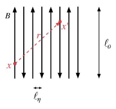
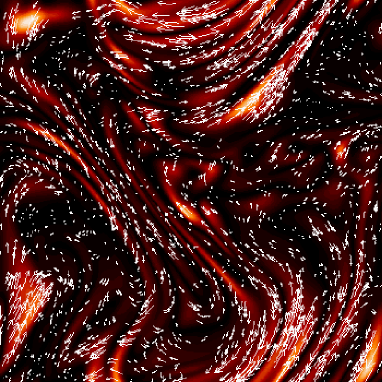
Figure 1: (a) The stripy field model. (b) A cross section of $|\boldsymbol{B}|$ for the run used in figure 2(a) ($\mbox{Pm}=1250$). Arrows indicate the in-plane direction of the field.

3.3 The $4/3$ law and the stripy-field model

The $4/3$ law, equation (8), is more interesting. In terms of $\delta\boldsymbol{u}$ and $\delta\boldsymbol{B}$, it reads

$$\left<\delta z_{L}^{\mp}|\delta\boldsymbol{z}^{\pm}|^{2}\right> = \left<\delta u_{L}|\delta\boldsymbol{u}|^{2}\right>\pm 2\left<\delta u_{L}\delta\boldsymbol{u}\cdot\delta\boldsymbol{B}\right>\mp\left<\delta B_{L}|\delta\boldsymbol{u}^{2}|\right>$$ (12)

$$+\,\,\left<\delta u_{L}|\delta\boldsymbol{B}|^{2}\right>-2\left<\delta B_{L}\delta\boldsymbol{u}\cdot\delta\boldsymbol{B}\right>\mp\left<\delta B_{L}|\delta\boldsymbol{B}|^{2}\right>$$

$$= -{4\over 3}\,\epsilon r+2\frac{\partial}{\partial r}\left[\nu\left<|\delta\boldsymbol{u}|^{2}\right>\pm(\nu+\eta)\left<\delta\boldsymbol{u}\cdot\delta\boldsymbol{B}\right>+\eta\left<|\delta\boldsymbol{B}|^{2}\right>\right].$$

Since $\delta\boldsymbol{u}\sim r$, the first term on the left-hand side is $\sim r^{3}$, the second and third terms are $\sim r^{2}$, so all three are subdominant and can be dropped. The remaining terms depend on the structure of the magnetic field. Let us consider a drastically simplified model of this structure based on the understanding that the field is organised in folds with direction reversals at the resistive scale. The model is illustrated in figure 1(a). The orientation of $\boldsymbol{B}$ on this sketch must be understood as one among many possible orientations with equal probability, since the flow is statistically isotropic. The field is taken to be straight (or coherent along itself on scales comparable to the forcing scale $\ell_{0}$) and to oscillate rapidly with spatial period $2\ell_{\eta}\ll\ell_{0}$ across itself. Given an arbitrary point $\boldsymbol{x}$, if we randomly pick a point $\boldsymbol{x}^{\prime}$ on a sphere centered at $\boldsymbol{x}$ with a fixed radius $r$ such that $\ell_{\eta}\ll r\ll\ell_{\nu}$, the field increment will be $\delta\boldsymbol{B}=-2\boldsymbol{B}(\boldsymbol{x})$ with probability $1/2$ and $\delta\boldsymbol{B}=0$ with probability $1/2$. We may now use this simple model and $\left<\hat{r}_{i}\hat{r}_{j}\right>=(1/3)\delta_{ij}$ to calculate

$$\left<\delta u_{L}|\delta\boldsymbol{B}|^{2}\right> = 2\left<B^{2}\nabla_{i}u_{j}\right>\left<\hat{r}_{i}\hat{r}_{j}\right>r={2\over 3}\left<B^{2}\boldsymbol{\nabla}\cdot\boldsymbol{u}\right>r=0,$$ (13)

$$2\left<\delta B_{L}\delta\boldsymbol{u}\cdot\delta\boldsymbol{B}\right> = 4\left<B_{i}B_{j}\nabla_{k}u_{j}\right>\left<\hat{r}_{i}\hat{r}_{k}\right>r={4\over 3}\left<\boldsymbol{B}\boldsymbol{B}:\boldsymbol{\nabla}\boldsymbol{u}\right>r,$$ (14)

$$\left<\delta B_{L}|\delta\boldsymbol{B}|^{2}\right> = -4\left<B^{2}B_{i}\right>\left<\hat{r}_{i}\right>=0,$$ (15)

$$\left<|\delta\boldsymbol{u}|^{2}\right> = \left<\nabla_{i}u_{j}\nabla_{k}u_{j}\right>\left<\hat{r}_{i}\hat{r}_{k}\right>r^{2}={1\over 3}\left<|\boldsymbol{\nabla}\boldsymbol{u}|^{2}\right>r^{2},$$ (16)

$$\left<\delta\boldsymbol{u}\cdot\delta\boldsymbol{B}\right> = -\left<B_{i}\nabla_{j}u_{i}\right>\left<\hat{r}_{j}\right>r=0,$$ (17)

$$\left<|\delta\boldsymbol{B}|^{2}\right> = 2\left<B^{2}\right>.$$ (18)

Substituting these expressions into equation (12), we see that it reduces to the power balance (11) just as the $4/5$ law did. It is essential, however, that to achieve this seemingly trivial outcome, we had to make assumptions about the spatial structure of the magnetic field. We have thus shown that a stripy alternating field is consistent with the $4/3$ law.

It is perhaps appropriate to stress that the stripy field sketched in figure 1(a) is a highly idealised model of the field structure that does not take into account, for example, such features as turning points, bending of the folds on the scale of the flow, the extent to which the stripes are volume filling, possibility of some degree of misalignment of the alternating fields, etc. However, it has allowed us to give a particularly simple demonstration of the way the $4/3$ law accommodates the folded magnetic fields evident in figure 1(b). The key to understanding why such a simple model appears to be sufficient at least on the qualitative level may be that the fields best described by this model are also the strongest ones, so the model captures well the statistical quantities weighed towards the parts of the system where the field strength is largest.

4 Numerical Tests

We now consider how equations (6) and (8) are satisfied in numerical experiments. We use the data from direct numerical simulations of isotropic MHD turbulence by Schekochihin et al. (2004). The list of runs and other details are provided in that paper. These are three-dimensional spectral simulations in a periodic cube of size 1. They employ a white-noise random forcing at the box scale. The average power input is $\epsilon=1$.

4.1 The averaging procedure

We use three levels of averaging to obtain two-point correlation and structure functions.

• Spherical average. For a given point $\boldsymbol{x}$ and a given point separation $r$, we average over all possible orientations of $\boldsymbol{r}$. We use 200 discrete orientations. In order to obtain accurate results, it is necessary to resort to linear interpolation between grid points to compute the fields at $\boldsymbol{x}^{\prime}=\boldsymbol{x}+\boldsymbol{r}$. Using the spherical average ensures that spurious anisotropies introduced by finite size Cartesian grid effects are filtered out. It is not restrictive, because the turbulence is statistically isotropic.

• Volume average. Since the turbulence is spatially homogeneous, we average over all points $\boldsymbol{x}$. In practice, the points $\boldsymbol{x}$ are picked on a submesh that is 10 times sparser than the mesh of the simulations.

• Time average. Finally, we average over about 20 box-crossing times. This is equivalent to averaging over many realisations of the turbulence. A relatively large number of independent snapshots is necessary in order to obtain converged correlation functions of odd power (see Rincon 2006). The averaged quantities we report are sufficiently converged (within a few percent for third-order quantities, which have the slowest convergence rate) for a qualitative understanding of the scale-by-scale budgets. We do not attempt any high-precision determination of scaling exponents from this data.

Note that in computing the two-point statistical quantities, we may only use points $\boldsymbol{x}^{\prime}$ within a radius $r$ up to 1/4 of the box size from any given point $\boldsymbol{x}$ because at larger distances spurious correlations arise due to the periodicity of the box.

4.2 Numerical results in the viscosity-dominated limit

It is not currently possible to have a resolved numerical simulation with $\mbox{Pm}\gg 1$ and $\mbox{Re}\gg 1$. However, one can study the subviscous fields in numerical simulations with $\mbox{Pm}\gg 1$ and $\mbox{Re}\sim 1$ (the viscosity-dominated limit; see Schekochihin et al., 2004). This means that the inertial range physics is sacrificed and we study the saturated state of a small-scale dynamo with $\mbox{Rm}\gg 1$ and a single-scale ($\sim\ell_{0}$) randomly forced flow. We note that in this setting, the difference between the Batchelor (1950) and Schlüter & Biermann (1950) scenarios of saturation mentioned in §3.1 cannot be detected.

Since the viscosity is large, the flow is smooth at all scales. As we explained in §3.2, the $4/5$ law in this regime does not contain any information beyond the power balance (11). Numerical results are in line with this expectation (not shown). The consistency of the $4/3$ law is illustrated in figure 2(a), which shows that the left- and right-hand sides of equation (8) independently computed from the numerical data match each other. The deviations at large scales are due to the higher-order terms in the Taylor expansion $\left<\boldsymbol{f}\cdot\boldsymbol{u}^{\prime}\right>=\epsilon+O(r^{2}/\ell_{0}^{2})$. In equation (8), the dominant term in the left-hand side is the viscous one. However, for a smooth velocity field, it is linear in $r$ (equation (16)), and, indeed, we find that the third-order structure function $-\left<\delta z_{L}^{-}|\delta\boldsymbol{z}^{+}|^{2}\right>\simeq(4/3)\left(\epsilon-\nu\left<|\boldsymbol{\nabla}\boldsymbol{u}|^{2}\right>\right)r$ is also linear in $r$ for $r\gtrsim\ell_{\eta}$. The main contribution to it is due to $2\left<\delta B_{L}\delta\boldsymbol{u}\cdot\delta\boldsymbol{B}\right>$, while all other terms in the left-hand side of equation (12) are subdominant. This is consistent with what is predicted by the stripy-field model, equations (13)–(15), although equation (14) is only satisfied approximately (within $\sim 30\%$). Note that for $r\ll\ell_{\eta}$, the magnetic field is smooth, $\delta\boldsymbol{B}\sim r$, so the transition from the subresistive scaling $\left<\delta z_{L}^{-}|\delta\boldsymbol{z}^{+}|^{2}\right>\sim r^{3}$ to $\left<\delta z_{L}^{-}|\delta\boldsymbol{z}^{+}|^{2}\right>\sim r$ shows what the effective magnitude of the resistive scale is: $\ell_{\eta}\sim 0.03$ for the run used in figure 2(a).

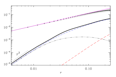
Figure 2: (a) The $4/3$ law for a run with $\mbox{Pm}=1250$, $\mbox{Re}\sim 1$ (run S5 of Schekochihin et al. 2004: $256^{3}$, $\nu=5\times 10^{-2}$, $\eta=4\times 10^{-5}$). We plot minus the left- (+++) and the right-hand (—) sides of equation (8), and also minus the dissipative term ($\cdot\cdot\cdot$). Several individual third-order structure functions in the left-hand side of equation (12) are shown: $-\left<\delta z_{L}^{-}|\delta\boldsymbol{z}|^{2}\right>$ (——), $2\left<\delta B_{L}\delta\boldsymbol{B}\cdot\delta\boldsymbol{u}\right>$ ($-\cdot-$), $-\left<\delta u_{L}|\delta\boldsymbol{u}|^{2}\right>$ ($---$), $-\left<\delta u_{L}|\delta\boldsymbol{B}|^{2}\right>$ ($-\cdot\cdot\cdot-$). The three functions that are not shown are small. (b) The second-order structure function $\left<|\delta\boldsymbol{B}|^{2}\right>/2\left<B^{2}\right>$ for a sequence of runs with increasing Pm and constant $\mbox{Re}\sim 1$ (runs S1–S6 of Schekochihin et al. 2004).

4.3 Scaling of the magnetic-field increments and the magnetic-energy spectrum

The stripy-field model implies that $\delta B(r)\sim B_{\rm rms}={\rm const}$ for $\ell_{\eta}\ll r\ll\ell_{\nu}$ (equation (18)). Note that $\left<|\delta\boldsymbol{B}|^{2}\right>\to 2\left<B^{2}\right>$ in the limit $r\to\infty$ for any field structure, as long as the field decorrelates at long distances, $\left<\boldsymbol{B}^{\prime}\cdot\boldsymbol{B}\right>\to 0$. The nontrivial property of the stripy-field model is that this value is reached already at $r\gtrsim\ell_{\eta}$ because $\left<\boldsymbol{B}^{\prime}\cdot\boldsymbol{B}\right>=0$ due to direction reversals. Figure 2(b) shows that the scale at which the value $\left<|\delta\boldsymbol{B}|^{2}\right>\simeq 2\left<B^{2}\right>$ is reached does indeed decrease as Rm is increased.

What the magnetic-energy spectrum is in the saturated state is not currently known. The stripy-field result $\delta B\sim r^{0}$ appears to imply that the spectrum is $k^{-1}$. However, the stripy-field model does not take into account that the alternating fields do not cancel each other perfectly, so there should be a gradual loss of correlation as $r$ increases. If this effect is important, the correlation function $\left<|\delta\boldsymbol{B}|^{2}\right>$ may have a peak around $r\sim\ell_{\eta}$ followed by a gradual fall off to the value $2\left<B^{2}\right>$ at $r\gg\ell_{\eta}$. If this fall off is a power law $\sim(\ell_{\eta}/r)^{1+\alpha}$, the spectrum should then be $k^{\alpha}$. For example, in the kinematic regime of the small-scale dynamo, theory predicts $\alpha=3/2$ (Kazantsev, 1968). In the saturated state, the numerically computed correlation functions (figure 2(b)) show no sign of having a peak, which suggests $\alpha=-1$. It cannot, however, be ruled out that, as suggested in Schekochihin et al. (2004), the spectrum is flatter, possibly even $\alpha>0$, but the convergence to the asymptotic scalings is slow and the values of Pm used in our simulations are insufficient to determine $\alpha$ accurately.

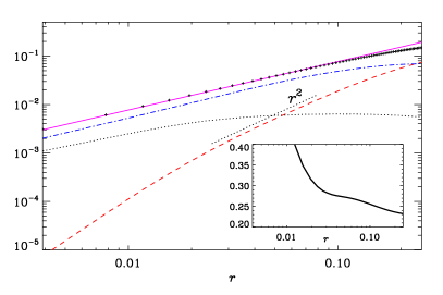
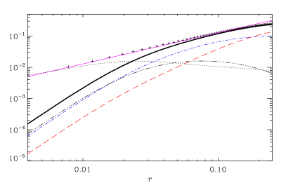
Figure 3: (a) The $4/5$ law for a run with $\mbox{Pm}=1$, $\mbox{Re}\simeq 400$ (run A of Schekochihin et al. 2004: $256^{3}$, $\nu=\eta=5\times 10^{-4}$). We plot minus the left- (+++) and the right-hand (—) sides of equation (6), minus the viscous term ($\cdot\cdot\cdot$), $-\left<\delta u_{L}^{3}\right>$ ($---$) and $6\left<B_{L}^{2}\delta u_{L}\right>$ ($-\cdot-$). Inset: plot of $\ell_{*}=-6\left<B_{L}^{2}\delta u_{L}\right>r/\left<\delta u_{L}^{3}\right>$. (b) The $4/3$ law for the same run. See caption of figure 2(a) for explanation of line styles. The functions $\left<\delta u_{L}\delta\boldsymbol{u}\cdot\delta\boldsymbol{B}\right>$, $\left<\delta B_{L}|\delta\boldsymbol{u}|^{2}\right>$ and $\left<\delta B_{L}|\delta\boldsymbol{B}|^{2}\right>$ are again small (not shown).

4.4 Numerical results for $\mbox{Pm}=1$

While the limit $\mbox{Rm}\gg\mbox{Re}\gg 1$ is unresolvable, some idea of the structure of isotropic MHD turbulence in a regime that is not viscosity-dominated can be gained by studying the case of $\mbox{Pm}=1$, which has been the favourite choice in numerical experiments (e.g., Haugen et al., 2004). Such simulations may, in fact, be more relevant than it would appear to understanding the $\mbox{Pm}\gg 1$ regime if the saturated state of the small-scale dynamo is controlled by the interaction of the folded magnetic fields with the forcing-scale velocities (§3.1), rather than — as Batchelor (1950) thought — with the viscous-scale ones.

Whether this is true is best addressed numerically by comparing the four terms in the $4/5$ law, equation (6). This is done in figure 3(a) for a run with $\mbox{Re}=\mbox{Rm}\simeq 400$. The $4/5$ law is well satisfied: the independently computed left- and right-hand sides of equation (6) match except for the large-scale discrepancy due to the higher-order contributions from the forcing term. The viscous term is subdominant for $r\gtrsim\ell_{\nu}\simeq 0.05$ leaving some room for a possible inertial range. Except at $r\sim\ell_{0}$, the dominant balance is between $6\left<B_{L}^{2}\delta u_{L}\right>$ and $(4/5)\epsilon r$, while $\left<\delta u_{L}^{3}\right>$ is subdominant. Physically this means that the kinetic-energy cascade is short-circuited by the energy transfer into the magnetic field. Interestingly, for the subdominant “cascade” term, we find empirically

$$-\left<\delta u_{L}^{3}\right>\simeq 6\left<B_{L}^{2}\delta u_{L}\right>{r\over\ell_{*}}\simeq{4\over 5}{\epsilon\over\ell_{*}}\,r^{2},$$ (19)

where $\ell_{*}\simeq 0.25$ is some typical length, comparable to the forcing scale $\ell_{0}$. The resolution is limited and the scale range where $\left<\delta u_{L}^{3}\right>\propto r^{2}$ holds is not wide. Numerically, the relation $\left<\delta u_{L}^{3}\right>\propto\left<B_{L}^{2}\delta u_{L}\right>r$ turns out to be satisfied across a somewhat wider interval (see inset in figure 3(a)). Equation (19) suggests that the velocity increments have the scaling $\delta u\sim r^{2/3}$. Indeed, the second-order structure function of $\boldsymbol{u}$ computed from our data is consistent with $\left<\delta u_{L}^{2}\right>\sim r^{4/3}$ (not shown) and the kinetic-energy spectrum does appear to have the corresponding scaling $k^{-7/3}$, as noticed by Schekochihin et al. (2004).

The $4/3$ law is well satisfied (figure 3(b)), as it was in the viscosity-dominated case (§4.2), but now there is an interval ($r\gtrsim 0.02$) where the dissipative terms are small and equation (8) becomes $-\left<\delta z_{L}^{-}|\delta\boldsymbol{z}^{+}|^{2}\right>\simeq(4/3)\epsilon r$. The numerically computed third-order structure function in the right-hand side of this equation does, indeed, scale linearly with $r$. The main contribution to this function still comes from $2\left<\delta B_{L}\delta\boldsymbol{u}\cdot\delta\boldsymbol{B}\right>$ (see equation (12)), except at the largest scales, where $\left<\delta u_{L}|\delta\boldsymbol{u}|^{2}\right>$ becomes important. That the $4/3$ law approximately reduces to a balance between the magnetic-interaction term $2\left<\delta B_{L}\delta\boldsymbol{u}\cdot\delta\boldsymbol{B}\right>$ and $(4/3)\epsilon r$ with the kinetic-energy “cascade” term $\left<\delta u_{L}|\delta\boldsymbol{u}|^{2}\right>$ interfering only at $r\sim\ell_{0}$ is in line with what we learned above from the $4/5$ law. The qualitative similarity of the internal structure of $\left<\delta z_{L}^{-}|\delta\boldsymbol{z}^{+}|^{2}\right>$ (the relative importance of the six terms in the left-hand side of equation (12)) to the viscosity-dominated case appears to suggest that the magnetic field in the $\mbox{Pm}=1$ case still has a stripy (folded) structure. This is, indeed, supported by various quantitative tests (Schekochihin et al., 2004).

5 Discussion: turbulence in the presence of stripy field

Numerical results appear to make a fairly compelling case that the structure of the magnetic field in the isotropic MHD turbulence is dominated by folds (stripes). We have demonstrated above that such a structure is consistent with the exact scaling laws. It has proven to be much more difficult to understand the structure of the velocity field. It is clear that the cascade of kinetic energy is short-circuited at the forcing scale, with injected energy diverted into maintaining the folds against continuous Ohmic dissipation. It is not clear from the available numerical results whether most or only a finite fraction of the injected power $\epsilon$ is thus diverted. If the latter is the case, i.e., if the magnetic-interaction term $6\left<B_{L}^{2}\delta u_{L}\right>$ only cancels a part of the flux term $(4/5)\epsilon r$ in equation (6), there should still be a kinetic-energy cascade from the forcing to viscous scale and it is hard to see from equation (6) how the velocity increments associated with this cascade can fail to have the Kolmogorov scaling, $\left<\delta u_{L}^{3}\right>\simeq-(4/5)\chi\epsilon r$, where $\chi<1$ is some finite positive number. These motions are likely to be Alfvénic perturbations of the folded structure (Schekochihin et al., 2002). If, on the other hand, the short-circuiting of the kinetic-energy cascade is nearly complete, i.e., $6\left<B_{L}^{2}\delta u_{L}\right>\simeq(4/5)\epsilon r$, then a subdominant scaling is possible: $\left<\delta u_{L}^{3}\right>\sim r^{\beta}$, $\beta>1$. Equation (19), which we deduced from our numerical experiment, appears to support this possibility with $\beta=2$. However, the resolution of our study was not sufficient to have a convincing parameter scan in Re and prove that the steeper-than-Kolmogorov scaling of the velocity increments is not simply due to too much viscosity. Note that Haugen et al. (2004) report kinetic-energy spectra that may be consistent with $k^{-5/3}$ at values of Re roughly twice as large as ours.

We remark in passing that the short-circuiting of the kinetic-energy cascade appears also to be a feature of the turbulence in polymer solutions (De Angelis et al., 2005; Berti et al., 2006), the mathematical description of which is similar to MHD, with elastic polymer chains stretched by turbulence in the same way magnetic fields are.

While the above study does not constitute the complete solution of the problem of isotropic MHD turbulence, it adds to the weight of evidence that this turbulence is controlled by the direct nonlocal interaction between the forcing-scale motions and small-scale stripy, or folded, magnetic structures. This nonlocality means that scaling arguments cannot be made along the usual, Kolmogorov-like, lines. This makes the problem conceptually difficult. The numerical simulations, while helpful, are not as yet sufficiently large to access the asymptotic regime of interest: ideally, $\mbox{Rm}\gg\mbox{Re}\gg 1$. The exact scaling laws provide the only rigorous quantitative constraints available in the theory of turbulence and are, therefore, useful. In this paper, we have attempted to discern the message that these laws carry about the structure of isotropic MHD turbulence. Given the limited resolution of the numerical experiments that we used to guide us, it may be fruitful to return to this type of analysis when larger computations become feasible.