Rapid-Response Mode VLT/UVES spectroscopy of GRB 060418

We present high-resolution spectroscopic observations of GRB 060418, obtained with VLT/UVES. These observations were triggered using the VLT Rapid-Response Mode (RRM), which allows for automated observations of transient phenomena, without any human intervention. This resulted in the first UVES exposure of GRB 060418 to be started only 10 minutes after the initial Swift satellite trigger. A sequence of spectra covering 330-670 nm were acquired at 11, 16, 25, 41 and 71 minutes (mid-exposure) after the trigger, with a resolving power of 7 km s^-1, and a signal-to-noise ratio of 10-15. This time-series clearly shows evidence for time variability of allowed transitions involving Fe II fine-structure levels (⁶D_7/2, ⁶D_5/2, ⁶D_3/2, and ⁶D_1/2), and metastable levels of both Fe II (⁴F_9/2 and ⁴D_7/2) and Ni II (⁴F_9/2), at the host-galaxy redshift $z=1.490$. This is the first report of absorption lines arising from metastable levels of Fe II and Ni II along any GRB sightline. We model the observed evolution of the level populations with three different excitation mechanisms: collisions, excitation by infra-red photons, and fluorescence following excitation by ultraviolet photons. Our data allow us to reject the collisional and IR excitation scenarios with high confidence. The UV pumping model, in which the GRB afterglow UV photons excite a cloud of atoms with a column density $N$, distance $d$, and Doppler broadening parameter $b$, provides an excellent fit, with best-fit values: log $N$(Fe II)=$14.75^{+0.06}_{-0.04}$, log $N$(Ni II)=$13.84\pm 0.02$, $d=1.7\pm 0.2$ kpc (but see Appendix A), and $b=25\pm 3$ km s^-1. The success of our UV pumping modeling implies that no significant amount of Fe II or Ni II is present at distances smaller than $\sim$1.7 kpc (but see erratum in Appendix A), most likely because it is ionized by the GRB X-ray/UV flash. Because neutral hydrogen is more easily ionized than Fe II and Ni II, this minimum distance also applies to any H I present. Therefore the majority of very large H I column densities typically observed along GRB sightlines may not be located in the immediate environment of the GRB. The UV pumping fit also constrains two GRB afterglow parameters: the spectral slope, $\beta=$$-0.5^{+0.8}_{-1.0}$, and the total rest-frame UV flux that irradiated the cloud since the GRB trigger, constraining the magnitude of a possible UV flash.

Table 1: Log of UVES observations

$$\begin{array}[]{cccrclrcccr}\hline\cr\hline\cr\vskip 3.0pt plus 1.0pt minus 1.0pt\cr\rm UT\,start&\rm epoch&\rm Fig.\leavevmode\nobreak\ \ref{fig:profiles}\leavevmode\nobreak\ line\leavevmode\nobreak\ colour&\rm\Delta T^{a}&\lambda_{\rm central}&\rm coverage&\rm exptime&\rm seeing^{b}&\rm FWHM&\rm S/N&\rm OT\,mag^{c}\\ \rm(2006\,April\,18)&&&\rm(min)&\rm(nm)&\rm(nm)&\rm(min)&\rm(\arcsec)&($km s$^{-1}$$)&\rm peak&\\ \hline\cr$3:16:07$&1&\rm black&11.47&390&328$-$452&3&1.5&6.9&6&\rm R\leavevmode\nobreak\ (6min)=14.0\\ $3:16:02$&1&&11.38&564&462$-$560;568$-$665&3&1.1&7.2&14&\rm V\leavevmode\nobreak\ (6.5min)=15.0\\ $3:20:17$&2&\rm red&16.61&390&328$-$452&5&1.5&6.9&6&\rm z\leavevmode\nobreak\ (16.3min)=14.4\\ $3:20:12$&2&&16.52&564&462$-$560;568$-$665&5&1.0&7.2&15&\\ $3:26:27$&3&\rm blue&25.13&390&328$-$452&10&1.5&6.9&7&\\ $3:26:17$&3&&24.96&564&462$-$560;568$-$665&10&1.0&7.2&16&\\ $3:38:01$&4&\rm green&41.20&390&328$-$452&20&1.4&6.9&7&\\ $3:37:56$&4&&41.12&564&462$-$560;568$-$665&20&0.9&7.2&17&\\ $3:59:30$&5&\rm magenta&70.99&390&328$-$452&40&1.4&6.9&7&\rm I\leavevmode\nobreak\ (69min)=16.5\\ $3:59:24$&5&&70.88&564&462$-$560;568$-$665&40&0.9&7.2&17&\rm z\leavevmode\nobreak\ (78min)=16.2\\ $4:41:51$&6&&128.09&437&376$-$498&80&1.0&6.1&9&\rm V\leavevmode\nobreak\ (100min)=18.8\\ $4:41:46$&6&&128.00&860&670$-$852;866$-$1043&80&0.8&6.5&21&\rm I\leavevmode\nobreak\ (135min)=17.4\\ \hline\cr\end{array}$$

1 Introduction

The influence of a $\gamma$-ray burst (GRB) explosion on its environment has been predicted to manifest itself in various ways. Strong observational evidence (Galama et al. 1998; Stanek et al. 2003; Hjorth et al. 2003) indicates that at least some GRB progenitors are massive stars (Woosley 1993; MacFadyen & Woosley 1999), and therefore the explosion is likely to take place in a star-forming region. As the GRB radiation ionizes the atoms in the environment, the neutral hydrogen and metal column densities in the vicinity of the explosion are expected to evolve with time (Perna & Loeb 1998; Vreeswijk et al. 2001; Mirabal et al. 2002). Ultra-violet (UV) photons will not only photo-dissociate and photo-ionize any nearby molecular hydrogen, but also quickly excite H₂ at larger distances to its vibrationally excited metastable levels, which can be observed in absorption (Draine & Hao 2002). Finally, dust grains can be destroyed up to tens of parsecs away (Waxman & Draine 2000; Fruchter et al. 2001; Draine & Hao 2002; Perna & Lazzati 2002; Perna et al. 2003). Detection of these time-dependent processes, with timescales ranging from seconds to days in the observer’s frame, would not only provide direct information on the physical conditions of the interstellar medium (ISM) surrounding the GRB, but would also constrain the properties of the emitted GRB flux before it is attenuated by foreground absorbers in the host galaxy and in intervening gas clouds. In the X-ray, evidence has been found for a time-variable H I column density (Starling et al. 2005; Campana et al. 2007), presumably due to the ionization of the nearby neutral gas. In the optical, none of these processes have been observed until recently, when Dessauges-Zavadsky et al. (2006) reported a $\sim$3$\sigma$ variability detection of Fe II ⁶D_7/2 $\lambda$2396, observed at two epochs roughly 16 hours apart. Such observations are technically very challenging because high-resolution spectroscopy combined with the rapidly decaying afterglow flux requires immediate follow-up with 8-10 m class telescopes.

The Swift satellite, launched in November 2004, has permitted a revolution in rapid spectroscopic follow-up observations, providing accurate (5″) positions for the majority of GRBs within a few minutes of the GRB trigger. Numerous robotic imaging telescopes react impressively fast (within 10 sec) to Swift triggers. As for spectroscopic observations, a number of target-of-opportunity programs at most major observational facilities are regularly yielding follow-up observations of the GRB afterglow at typically an hour after the Swift alert. However, most of these programs require significant human coordination between the science team and telescope personnel/observers. At the European Southern Observatory’s (ESO) Very Large Telescope (VLT; consisting of four unit telescopes of 8.2 m each), a Rapid Response Mode (RRM) has been commissioned to provide prompt follow-up of transient phenomena, such as GRBs. The design of this system allows for completely automatic VLT observations without any human intervention except for the placement of the spectrograph entrance slit on the GRB afterglow. The typical time delay, which is mainly caused by the telescope preset and object acquisition, is 5-10 minutes, depending on the GRB location on the sky with respect to the telescope pointing position prior to the GRB alert. The data presented in this paper are the result of the first automatically-triggered RRM activation.

This paper is organized as follows: the UVES observations and data reduction are described in Sect. 2, followed by Sect. 3, in which we discuss general properties of the absorption systems at the host-galaxy redshift from the detection of resonance lines. In Sect. 4, we focus on the detection of variability of transitions originating from fine-structure levels of Fe II, and metastable levels of Fe II and Ni II. The time evolution of the level population of these excited levels is modeled in Sect. 5. The results and their implications are discussed in Sect. 6, and we conclude in Sect. 7.

2 UVES observations and data reduction

On April 18 2006 at 3:06:08 UT the Swift Burst Alert Telescope (BAT) triggered a $\gamma$-ray burst alert (Falcone et al. 2006a), providing a 3′ error circle localization. Observations with the Swift X-Ray Telescope (XRT) resulted in a 5″ position about one minute later (Falcone et al. 2006b), which triggered our desktop computer to activate a VLT-RRM request for observations with the Ultra-violet and Visual Echelle Spectrograph (UVES). This was received by the VLT’s unit telescope Kueyen at Cerro Paranal at 3:08:12 UT. The on-going service mode exposure was ended immediately, and the telescope was pointed to the XRT location, all automatically. Several minutes later, the night astronomers Stefano Bagnulo and Stan Stefl identified the GRB afterglow, aligned the UVES slit on top of it, and started the requested observations at 3:16 UT (i.e. 10 minutes after the Swift $\gamma$-ray detection). This represents the fastest spectral follow-up of any GRB by an optical facility (until the RRM VLT/UVES observations of GRB 060607, also triggered by our team, which were started at a mere 7.5 minutes after the GRB; Ledoux et al. 2006). A series of exposures with increasing integration times (3, 5, 10, 20, and 40 minutes, respectively) was performed with a slit width of 1″, yielding spectra covering the 330–670 nm wavelength range at a resolving power of $R=\Delta\lambda/\lambda$ $\sim$ 43,000, corresponding to 7 km s^-1 full width at half maximum. These observations were followed by a 80-minutes exposure in a different instrument configuration, but with the same slit width, extending the wavelength coverage to the red up to 950 nm. The data were reduced with a custom version of the UVES pipeline (Ballester et al. 2000), flux-calibrated using the standard response curves and converted to a heliocentric vacuum wavelength scale. The log of the observations is shown in Table 1.

Table 2: Ionic column densities and abundance ratios in the combined spectrum (see Fig.1 for the corresponding profile fits).

$$\begin{array}[]{llrrrr}\hline\cr\hline\cr\rm Ion&\rm Lines\,\,used&\lx@intercol\hfil\log\leavevmode\nobreak\ N\pm\sigma_{\log\leavevmode\nobreak\ N}$$^{\rm a}$$\hfil\lx@intercol\\ \hline\cr\rm component&&1&2&3&\rm total\\ z$$_{\rm abs}$$&&1.49001(1)&1.48999(7)&1.49018(3)&\\ b\leavevmode\nobreak\ ($km s$^{-1}$$)&&23.6\pm 0.4&3.0\pm 0.4&6.5\pm 0.1&\\ \hline\cr\rm C\leavevmode\nobreak\ I&1656&12.52\pm 0.18&12.29\pm 0.14&12.19\pm 0.17&12.83\pm 0.11\\ \rm Mg\leavevmode\nobreak\ I&2026&<12.07&13.01\pm 0.02&13.60\pm 0.01$$^{\rm b}$$&13.70\pm 0.02$$^{\rm b}$$\\ \rm Si\leavevmode\nobreak\ II&1808&15.74\pm 0.02&14.85\pm 0.17&15.34\pm 0.05&15.92\pm 0.03\\ \rm Cr\leavevmode\nobreak\ II&2056,2062,2066&13.51\pm 0.01&12.46\pm 0.06&12.88\pm 0.03&13.63\pm 0.02\\ \rm Mn\leavevmode\nobreak\ II&2576,2594,2606&12.97\pm 0.01&11.82\pm 0.05&12.59\pm 0.02&13.14\pm 0.01\\ \rm Fe\leavevmode\nobreak\ II&1611&14.88\pm 0.10&14.03\pm 0.31&14.49\pm 0.11&15.07\pm 0.08\\ \rm Ni\leavevmode\nobreak\ II&1709,1741,1751&13.77\pm 0.03&12.82\pm 0.13&13.03\pm 0.08&13.88\pm 0.03\\ \rm Zn\leavevmode\nobreak\ II&2026,2062&12.80\pm 0.02&11.98\pm 0.05&12.69\pm 0.01&13.09\pm 0.01\\ \hline\cr\lx@intercol\rm Abundance\,\,ratio\hfil\lx@intercol\\ \rm[Si/Fe]&&0.79\pm 0.10&0.75\pm 0.35&0.78\pm 0.12&0.78\pm 0.09\\ \rm[Cr/Fe]&&0.45\pm 0.10&0.25\pm 0.32&0.21\pm 0.11&0.38\pm 0.08\\ \rm[Mn/Fe]&&0.06\pm 0.10&-0.24\pm 0.31&0.07\pm 0.11&0.04\pm 0.08\\ \rm[Ni/Fe]&&0.14\pm 0.10&0.04\pm 0.34&-0.21\pm 0.14&0.06\pm 0.09\\ \rm[Zn/Fe]&&0.76\pm 0.10&0.79\pm 0.31&1.04\pm 0.11&0.86\pm 0.08\\ \hline\cr\end{array}$$

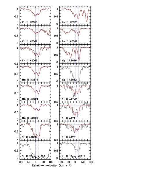
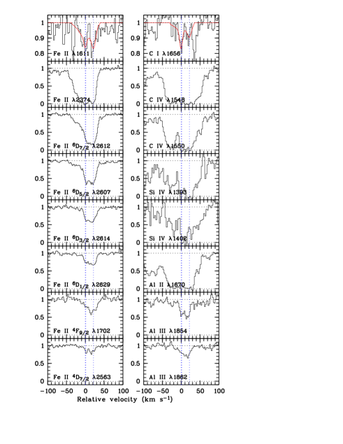
Figure 1: Absorption-line profiles for a variety of transitions detected at the GRB 060418 redshift. To all low-ionization species containing at least one non-saturated transition, we have performed simultaneous Voigt-profiles fits using a three-component model; the resulting fits are shown by the solid (red) line (see Table 2 for the fit results). The relative velocity of the different components are indicated by the (blue) vertical dotted lines; note that two components have very similar redshifts. It is clear that this 3-component fit does not describe some high S/N lines, such as Zn II $\lambda$2026, very well; we will come back to this in the discussion. We note, however, that the total column density would hardly change if additional components would be introduced. For comparison purposes, we also show transitions that we have not fit: (saturated) higher-ionization lines of C IV and Si IV, lines from Fe II fine-structure levels, and transitions originating from metastable levels of both Fe II and Ni II.

3 Ground-state absorption lines from the host galaxy of GRB 060418

The spectra reveal four strong absorption-line systems at redshifts $z=0.603,0.656,1.107$, and 1.490. In what follows, we focus on the highest-redshift absorption-line system at $z_{\rm abs}=1.490$, which corresponds to the redshift of the GRB as shown below; the intervening systems are discussed in a separate paper (Ellison et al. 2006).

At the redshift of the GRB host galaxy, we detect a large number of metal-absorption lines, arising from transitions involving the ground state of various ions (see below), fine-structure levels of Si II and Fe II, and metastable levels of Fe II and Ni II. We will discuss the excited-level lines in more detail in Sect. 4; in this section we focus on the resonance lines, i.e. lines corresponding to an allowed transition from the ion ground state to a higher excited level. The ions from which resonance lines are detected are C I, C IV, Cr II, Mn II, Si II, Si IV, Zn II, Mg I, Mg II, Ni II, Fe II, Al II, Al III, and Ca II. C II $\lambda$1334 is at the very blue edge of our spectrum, where the noise is dominating the signal. For Fe I, we determine an upper limit (5$\sigma$) on its column density of log N(Fe I)$<$11.48, using Fe I $\lambda$2484. A selection of lines is shown in Fig. 1. Because the resonance lines are not found to vary in time, we have combined all spectra (see Table 1) to achieve the highest signal-to-noise ratio (S/N) possible. The combined spectrum has S/N=16 at $\lambda$=4000 Å ($\lambda$_rest=1606 Å) and S/N=36 at $\lambda$=6500 Å ($\lambda$_rest=2610 Å). The redshift corresponding to the zero velocity has been adopted to be $z=1.49000$. At this redshift, the Ly$\alpha$ line is located at 3027 Å, just outside the UVES spectral range.

We now wish to highlight a number of observations that can be made from Fig. 1. The vast majority of the column density of the low- and high-ionization species (as well as fine-structure and metastable species) is located within a narrow range of velocity (with a spread of 50-100 km s^-1), and seems to be contained within two or three main components. This small range in velocity for the low-ionization species is also seen in GRB 051111 (Prochaska et al. 2006, 2007). Highly saturated lines such as those from C IV, Si IV, Mg II, and Al II show components to the blue up to $-200$ km s^-1, but these harbour only a small fraction of the total column density. The line profile of the high-ionization C IV lines follows the profile of the low-ionization lines very well, even though the comparison is made difficult by the fact that the C IV lines are much stronger. This similarity is uncommon in QSO-DLAs (Wolfe & Prochaska 2000). The main clump of the low-ionization line profiles, though kinematically simple, is a complex mix of broad and narrow components. Thanks to the high signal-to-noise ratio, a weak narrow component is clearly observed in the profiles of Cr II and Mn II at $-20$ km s^-1.

For a quantitative analysis, we have simultaneously fit Voigt-profiles (using the FITLYMAN context within MIDAS) to all resonance lines with at least one non-saturated transition. The atomic data required by the profile fits (vacuum wavelengths, oscillator strengths and damping coefficients) have been taken from Morton (2003). For the oscillator strengths of Ni II $\lambda$$\lambda$1709, 1741, and 1751, the values from Fedchak et al. (2000) have been adopted instead. We find that at least three components are required to yield an adequate fit to the data. Although a 3-component fit does not describe the blue side of a few high S/N lines perfectly (see e.g. Zn II $\lambda$2026 in Fig. 1), it is the simplest model that fits the data adequately. Adding a component on the blue side would also require an additional red component to compensate for the loss of the broad component on the red side; the redshift of this additional red component would be very hard to constrain. We note that the total column density derived would hardly change if more components are used. The redshift $z$ and the Doppler-broadening parameter $b$ (in km s^-1) for each component are assumed to be the same for all ions. Only for Mg I we had to tweak the redshift of the red component for a satisfactory fit. The slightly higher redshift for this component is reasonably consistent with the profile of Mg I $\lambda$2852, but it is more probable that the red Mg I component is blended. A third possibility is that there are two components in this red feature, where the reddest component would have a very high Mg I over Zn II ratio.

The best-fit redshifts and broadening parameters for each component are listed at the top of Table 2, along with the fit ionic column densities (individual and the total of all components). The fits are shown by the solid (red) line in Fig. 1. When comparing the resonance lines with the transitions from excited levels of Fe II and Ni II, it is apparent that although the profiles are very similar, the velocity spread of the latter is smaller. The one exception is Al III, whose red component (i.e. the one near +15 km s^-1) is not consistent with the resonance-line fit. The column densities that we find are consistent with those found by Prochaska et al. (2007), with the exception of Fe II, where our value of log N(Fe II)=$15.07\pm 0.08$ is lower (at 1.8$\sigma$ significance) than their adopted value of log N(Fe II)=$15.22\pm 0.03$. Prochaska et al. (2007) used the transitions Fe II $\lambda$2249 and $\lambda$2260, which are not saturated. In the UVES spectra these lines fall right in the red CCD gap, leaving us with one unsaturated line, Fe II $\lambda$1611, which has a lower oscillator strength. Therefore, we have more confidence in the determination by Prochaska et al. (2007); in the discussion that follows, it should be kept in mind that our total Fe II column density is probably too low by about 0.15 dex.

From the column densities we calculate the abundance ratios of several ions with respect to iron for each component separately and for the total, adopting the solar values from Lodders (2003). The resulting values are listed in Table 2. The ratio [Zn/Fe] is high compared to the global QSO-DLA population (Ledoux et al. 2003; Vladilo 2004), and suggests a large dust depletion, especially in component 3 where [Zn/Fe]=1.0. The solar value that we find for [Mn/Fe] provides additional evidence for substantial dust depletion (Ledoux et al. 2002; Herbert-Fort et al. 2006). Given these indications for a large dust depletion, the actual value for [Si/Zn] may be 0.2-0.3 dex higher than observed ([Si/Zn]${}_{\rm tot}=-0.08$), which would suggest an $\alpha$-element overabundance, provided that zinc can be used as a proxy for iron peak elements. Although the values for [Zn/Fe] and [Mn/Fe] are high compared to those found in QSO-DLAs ([Zn/Fe]_QSOs=0-1 and [Mn/Fe]_QSOs=$-$0.5-0.4), they are rather typical for the ISM of GRB host galaxies, with [Zn/Fe]_GRBs=1-2 and [Mn/Fe]_GRBs=0.1-0.3 (Savaglio et al. 2003; Savaglio & Fall 2004; Savaglio 2006). This dust depletion difference between QSO-DLAs and GRB host galaxies can be naturally explained if QSO sightlines on average do not probe the central regions of galaxies (for which there is growing evidence, e.g. Wolfe & Chen 2006; Ellison et al. 2005; Chen et al. 2005a), while GRB lines-of-sight do.

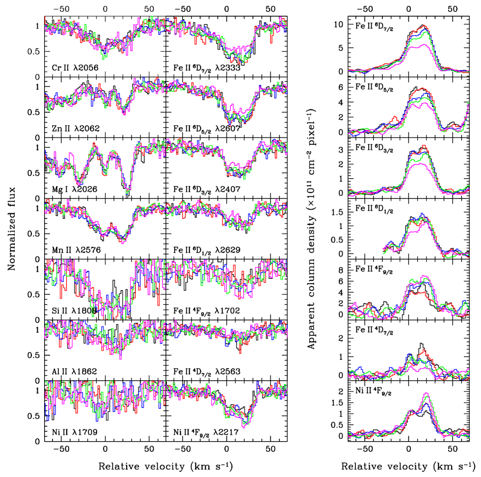
Figure 2: The epoch 1-5 UVES spectra of GRB 060418 (see Table 1) are overplotted with the colours black, red, blue, green and magenta, respectively. In the left panel individual lines are shown, typical resonance lines on the left, and the lines arising from the excited levels of Fe II and Ni II on the right. The latter show evidence for a varying equivalent width as a function of time. To make this variability clearer, we have combined various lines that arise from the same level and constructed apparent column density profiles, smoothed with a boxcar of 5 pixels; these are shown in the right panel.

Table 3: Column densities of the Fe II and Ni II excited levels, in the three individual components and the total, at the various epochs (see Table 1) since the burst trigger.

$$\begin{array}[]{cllll}\hline\cr\hline\cr\rm epoch&\lx@intercol\hfil\log\leavevmode\nobreak\ N\pm\sigma_{\log\leavevmode\nobreak\ N}$$^{\rm a}$$\hfil\lx@intercol\\ \hline\cr\rm comp.&1&2&3&\rm total\\ z$$_{\rm abs}$$&1.48996(6)&1.49002(4)&1.49015(9)&\\ b&28.0\pm 3.5&5.0\pm 2.1&10.2\pm 1.5&\\ \hline\cr&\lx@intercol\hfil\rm Fe\leavevmode\nobreak\ II\,^{6}{\rm D}_{7/2}\,$$\lambda$$\lambda$$2333,2383,2389,2612,2626\hfil\lx@intercol\\ 1&13.49\pm 0.02&13.27\pm 0.03&13.63\pm 0.02&13.96\pm 0.01\\ 2&13.52\pm 0.02&13.17\pm 0.03&13.64\pm 0.02&13.96\pm 0.01\\ 3&13.48\pm 0.02&13.14\pm 0.03&13.62\pm 0.02&13.93\pm 0.01\\ 4&13.37\pm 0.02&13.13\pm 0.03&13.57\pm 0.02&13.87\pm 0.01\\ 5&13.23\pm 0.03&13.06\pm 0.03&13.41\pm 0.02&13.73\pm 0.01\\ \hline\cr&\lx@intercol\hfil\rm Fe\leavevmode\nobreak\ II\,^{6}{\rm D}_{5/2}\,$$\lambda$$\lambda$$2328,2381,2399,2607,2618\hfil\lx@intercol\\ 1&13.09\pm 0.05&13.04\pm 0.03&13.45\pm 0.02&13.71\pm 0.02\\ 2&13.12\pm 0.04&13.06\pm 0.03&13.45\pm 0.02&13.72\pm 0.02\\ 3&13.12\pm 0.04&13.02\pm 0.03&13.39\pm 0.02&13.68\pm 0.02\\ 4&13.04\pm 0.04&12.96\pm 0.03&13.36\pm 0.02&13.63\pm 0.02\\ 5&12.84\pm 0.07&12.86\pm 0.04&13.24\pm 0.02&13.50\pm 0.02\\ \hline\cr&\lx@intercol\hfil\rm Fe\leavevmode\nobreak\ II\,^{6}{\rm D}_{3/2}\,$$\lambda$$\lambda$$2338,2359,2407,2411,2614,2621\hfil\lx@intercol\\ 1&12.60\pm 0.09&12.88\pm 0.03&13.17\pm 0.02&13.42\pm 0.02\\ 2&12.63\pm 0.08&12.85\pm 0.03&13.18\pm 0.02&13.42\pm 0.02\\ 3&12.59\pm 0.08&12.86\pm 0.03&13.18\pm 0.02&13.42\pm 0.02\\ 4&12.56\pm 0.08&12.78\pm 0.03&13.13\pm 0.02&13.36\pm 0.02\\ 5&12.38\pm 0.13&12.67\pm 0.04&13.00\pm 0.02&13.23\pm 0.03\\ \hline\cr&\lx@intercol\hfil\rm Fe\leavevmode\nobreak\ II\,^{6}{\rm D}_{1/2}\,$$\lambda$$\lambda$$2345,2411,2622,2629\hfil\lx@intercol\\ 1&12.38\pm 0.15&12.51\pm 0.06&12.77\pm 0.03&13.06\pm 0.04\\ 2&12.39\pm 0.14&12.42\pm 0.06&12.80\pm 0.03&13.06\pm 0.04\\ 3&12.65\pm 0.07&12.34\pm 0.07&12.77\pm 0.03&13.10\pm 0.03\\ 4&12.44\pm 0.10&12.42\pm 0.05&12.79\pm 0.03&13.06\pm 0.03\\ 5&12.35\pm 0.13&12.21\pm 0.08&12.73\pm 0.03&12.97\pm 0.04\\ \hline\cr&\lx@intercol\hfil\rm Fe\leavevmode\nobreak\ II\,^{4}{\rm F}_{9/2}\,$$\lambda$$\lambda$$1566$$^{\rm b}$$,1612$$^{\rm b}$$,1637$$^{\rm b}$$,1702$$^{\rm b}$$,2332,2360\hfil\lx@intercol\\ 1&12.74\pm 0.33&12.79\pm 0.14&13.17\pm 0.06&13.42\pm 0.10\\ 2&12.99\pm 0.17&12.62\pm 0.19&13.26\pm 0.05&13.51\pm 0.07\\ 3&12.91\pm 0.19&12.89\pm 0.10&13.40\pm 0.04&13.61\pm 0.05\\ 4&12.97\pm 0.15&13.09\pm 0.06&13.41\pm 0.03&13.68\pm 0.04\\ 5&12.54\pm 0.44&13.03\pm 0.07&13.47\pm 0.03&13.64\pm 0.06\\ 6&13.38\pm 0.12&12.53\pm 0.42&13.42\pm 0.07&13.73\pm 0.08\\ \hline\cr&\lx@intercol\hfil\rm Fe\leavevmode\nobreak\ II\,^{4}{\rm D}_{7/2}\,$$\lambda$$\lambda$$1635,2563\hfil\lx@intercol\\ 1&12.36\pm 0.30&12.35\pm 0.15&12.78\pm 0.06&13.02\pm 0.10\\ 2&12.33\pm 0.30&12.09\pm 0.25&12.75\pm 0.06&12.95\pm 0.11\\ 3&12.46\pm 0.20&12.35\pm 0.12&12.40\pm 0.12&12.88\pm 0.10\\ 4&11.35\pm 0.80&12.41\pm 0.10&12.49\pm 0.09&12.77\pm 0.10\\ 5&12.45\pm 0.20&11.54\pm 0.72&11.98\pm 0.30&12.61\pm 0.20\\ \hline\cr&\lx@intercol\hfil\rm Ni\leavevmode\nobreak\ II\,^{4}{\rm F}_{9/2}\,$$\lambda$$\lambda$$2166,2217,2223,2316\hfil\lx@intercol\\ 1&12.62\pm 0.11&12.59\pm 0.06&13.03\pm 0.03&13.27\pm 0.03\\ 2&12.83\pm 0.07&12.63\pm 0.06&13.10\pm 0.02&13.37\pm 0.03\\ 3&12.85\pm 0.06&12.66\pm 0.05&13.12\pm 0.02&13.40\pm 0.02\\ 4&12.82\pm 0.06&12.68\pm 0.05&13.22\pm 0.02&13.45\pm 0.02\\ 5&12.86\pm 0.06&12.61\pm 0.06&13.24\pm 0.02&13.46\pm 0.02\\ \hline\cr\end{array}$$

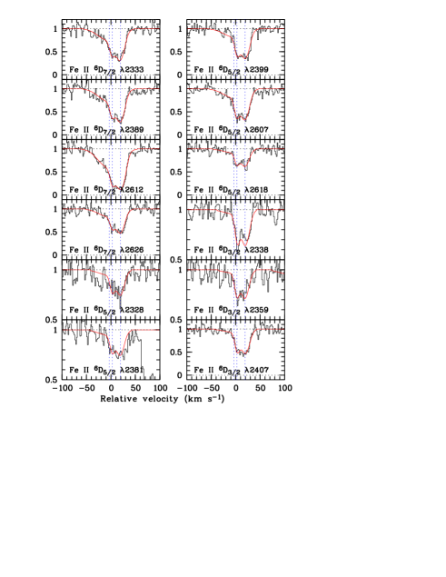
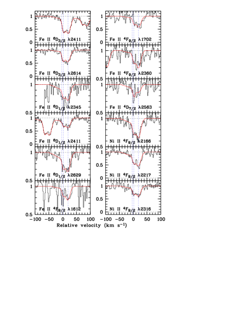
Figure 3: Absorption-line profile fits to selected transitions from excited Fe II and Ni II. The lower level of the transition, for which the column density is determined from the fits, is indicated in each panel. The fit results are listed in Table 3. We only show the fits for the third epoch spectra; the quality of the spectral fits for the other epochs are very similar, with only small differences due to slightly different signal-to-noise ratios (see Table 1).

4 Detection and variability of transitions involving excited levels of Fe II and Ni II

In the left panel of Fig. 2 we show the profiles of some selected resonance lines and transitions arising from all four fine-structure levels of Fe II (⁶D_7/2, ⁶D_5/2, ⁶D_3/2, and ⁶D_1/2), as well as from transitions from metastable levels of Fe II (⁴F_9/2 and ⁴D_7/2) and Ni II (⁴F_9/2). See Figs. 4 and 5 for an illustration of the relevant energetically lower levels of Fe II and Ni II, including the first higher excited level, and the wavelength and spontaneous decay probability of the transitions between the levels. Back to Fig. 2: we overplot the series of five spectra, epoch 1-5 (see Table 1), with the colours black, red, blue, green and magenta, respectively. Comparison of the two panels shows clear evidence for variability of the excited-level lines, while the strengths of the resonance lines are constant in time. To show this variability more clearly, we have constructed apparent column density profiles based on pixel optical depths in composite spectra (Savage & Sembach 1991) for each of the Fe II fine-structure levels and the Fe II and Ni II metastable levels; these profiles, which have been smoothed with a boxcar of 5 pixels, are shown in the right panel of Fig. 2.

We estimate the formal significance of this variability by measuring the equivalent width (EW) of the individual lines in between $-30$ km s^-1 and +40 km s^-1 at the various epochs, conservatively adding 3% of the EW to its formal error, due to the uncertainty in the placement of the continuum. Using the different EW values over the different epochs and its mean, we calculate the chi-square and the corresponding probability with which a constant equivalent width can be rejected. For the individual lines shown in Fig. 2: Fe II $\lambda$2333, Fe II $\lambda$2607, Fe II $\lambda$2407, Fe II $\lambda$2629, Fe II $\lambda$1702, Fe II $\lambda$2563, and Ni II $\lambda$2217, the significances are 4.5$\sigma$, 5.8$\sigma$, 2.1$\sigma$, 0.3$\sigma$, 2.5$\sigma$, 1.7$\sigma$, and 3.5$\sigma$, respectively. Using several transitions originating from the same level (the same that have been used to construct the apparent column density profiles in Fig. 2), we find the following numbers: 8.7$\sigma$ (Fe II ⁶D_7/2), 7.4$\sigma$ (Fe II ⁶D_5/2), 3.2$\sigma$ (Fe II ⁶D_3/2), 0.5$\sigma$ (Fe II ⁶D_1/2), 2.2$\sigma$ (Fe II ⁴F_9/2), 1.7$\sigma$ (Fe II ⁴D_7/2), and 2.5$\sigma$ (Ni II ⁴F_9/2).

We have performed Voigt-profile fitting to the lines originating from the excited levels of Fe II and Ni II, independent from the resonance-line fit. The atomic data from Morton (2003) were adopted when available, and if not we have assumed the values from Kurucz (2003) (note that for Ni II we have divided the Kurucz oscillator strengths by two; see the discussion in Sect. 5.2). The Voigt-profile fit results are shown in Table 3 and Fig. 3; we only show the fit profiles for epoch 3 as the other epochs display very similar results, but with somewhat different signal-to-noise ratios. Just as with the resonance lines, a satisfactory fit is found when using three components. In an initial fit, the redshift and $b$ parameter were free to vary from epoch to epoch. As these were found to be constant with time, in a final fit they were fixed to the averages over the five epochs; the $z$ and $b$ averages and the corresponding standard deviations are listed at the top of Table 3. The column density errors listed in Table 3 are the formal errors provided by FITLYMAN. We have also estimated an error in the placement of the continuum by varying the sigma clipping factors and the order of the polynomial with which we fit the continuum around each line, and rerun the Voigt profile fit. The maximum change that we find is 0.03 dex, which we add to the formal error for the rest of the analysis.

Prochaska et al. (2007) have performed time-resolved high-resolution spectroscopy of GRB 060418 as well. Their three spectra were taken around the same mid-exposure time as our epoch 4, 5 and 6 spectra. They do not consider variability, and report on the average column density for the four Fe II fine-structure levels; they do not mention the metastable levels of Fe II and Ni II. When comparing their average values with our epoch 4 column densities, the results are fully consistent within the errors.

Comparison of the resonance-lines fit with the excited-lines fit shows that the redshifts and $b$ parameters for the three components are very similar, cf. Tables 2 and 3. When we run the excited-lines profile fit with the redshift and $b$ parameter fixed at the values of the resonance lines, the resulting fit is very poor. Therefore, although the fits provide similar results, the redshifts and $b$ parameters are significantly different. We already noted this difference in Sect. 3, and we will come back to this point in Sect. 6.

Figure 4: Energy level diagram for selected levels of Fe II. For the lower levels we only show the levels for which we detect transitions, i.e. the fine-structure levels of the Fe II ground state, and ⁴F_9/2 and ⁴D_7/2. Note that for clarity reasons, we do not show the fine-structure levels of the latter. With the arrows, we indicate the most likely transitions between these levels, including one higher excited level. For each transition we show the wavelength in Å and the spontaneous decay Einstein coefficient, A_ul in s^-1 (which is proportional to the absorption coefficient B_lu, see also below). The electric dipole allowed transitions are indicated with a solid line, and the forbidden transitions (magnetic dipole or electric quadrupole) with a dotted line. Note that to populate the level ⁶D_1/2, either four IR photons are required, or two UV photons, where the higher levels involved need to have J=7/2 and J=3/2. This, combined with the much larger transition probabilities in the UV, makes the UV pumping mechanism much more efficient than IR excitation.

Figure 5: Energy level diagram for selected levels of Ni II (see Fig. 4). Note the very low A-value for the transition ⁴F_9/2 to the ground state (this is actually an electric quadrupole transition), while the level ⁴F_9/2 can be very easily populated from the higher excited levels, one of them being ⁴D${}^{\rm o}_{7/2}$. Therefore this level can be expected to be densely populated in the presence of a strong UV radiation field. The fine-structure level of Ni II ground state, ²D_3/2 has a relatively high probability of spontaneous decay, with a mean lifetime of 1/(5.4$\times 10^{-2}$ s^-1)=19 s.

Atomic fine-structure levels are caused by an energy split due to the interaction of the total electron spin and total angular momentum of the electrons. The transitions between these levels are not allowed, i.e. they cannot proceed through an electric dipole transition, and therefore the corresponding transition probabilities are low. The same is applicable to other energetically lower levels, also called metastable levels, and their fine-structure levels. Figures 4 and 5 show the energy level diagrams, of selected levels of Fe II and Ni II.

These fine-structure and metastable levels can be populated through (1) collisions between the ion and other particles such as free electrons, (2) direct photo-excitation by infra-red (IR) photons (with specific wavelengths between 87-260 $\mu$m), and/or (3) indirectly through excitation by ultra-violet (UV) photons, followed by fluorescence. Detection of transitions from these energetically lower excited levels provides a powerful probe of the physical conditions in the interstellar medium (Bahcall & Wolf 1968), where the quantities that can be derived depend on the excitation mechanism.

Vreeswijk et al. (2004) noted the presence of transitions originating from the fine-structure level of Si II in the host galaxy of GRB 030323; as these lines had never been clearly detected in QSO-DLAs (we note that they had been detected in absorption systems associated with the QSO, see Wampler et al. 1995; Srianand & Petitjean 2001), this detection suggested an origin in the vicinity of the GRB. Assuming that collisions with electrons were the dominant excitation mechanism, a volume density of n${}_{\rm HI}=10^{2}-10^{4}$ cm^-3 was derived (see also Savaglio & Fall 2004; Fynbo et al. 2006). We note that Si II ²P_3/2 $\lambda$1816 is not detected (5 $\sigma$ upper limit: log N$<$14.81) in the case of GRB 060418, and that Si II ²P_3/2 $\lambda$1533 (see Fig. 1) is severely blended with Fe II $\lambda$2382 at the redshift of an intervening absorber, $z=0.603$. Therefore, this (or any) Si II fine-structure level is not included in our analysis.

More recently, even more exotic transitions involving fine-structure levels of Fe II have been discovered in GRB sightlines (Chen et al. 2005b; Penprase et al. 2006; Prochaska et al. 2006; D’Elia et al. 2006). As noted by Prochaska et al. (2006), these lines had previously been detected in absorption in extreme environments such as Broad Absorption-Line (BAL) quasars (Hall et al. 2002), $\eta$ Carinae (Gull et al. 2005), and the disk of $\beta$ Pictoris (Lagrange-Henri et al. 1988). For the Fe II fine-structure level population along GRB sightlines it has been argued (Prochaska et al. 2006) that IR excitation is negligible, that collisional excitation is improbable (although not excluded), and that indirect UV pumping probably is the dominant excitation mechanism. The detection of variability at the 3$\sigma$ level (using two different instruments) of one Fe II fine-structure line in the spectrum of GRB 020813 was reported (Dessauges-Zavadsky et al. 2006), which the authors claim to be supportive evidence for the UV pumping model.

The lines arising from the metastable levels of both Fe II (⁴F_9/2 and ⁴D_7/2) and Ni II (⁴F_9/2) that we detect are the first lines from metastable levels to be identified along any GRB sightline. However, these have also been previously detected in BAL quasars (Hazard et al. 1987; Wampler et al. 1995) and $\eta$ Carinae (Gull et al. 2005).

Our clear detection of time-variation of numerous transitions involving all fine-structure levels of the Fe II ground state, and moreover transitions originating from metastable levels of Fe II and Ni II, allows for a critical comparison of the data with the three possible excitation mechanisms mentioned above. However, independent of the mechanism at play, the detection of time-variable absorption implies that the flux from the GRB prompt emission and/or afterglow, directly or indirectly, is the cause of the line variability, and that the absorbing atoms are located in the relative vicinity of the GRB explosion.

5 Modeling of the time evolution of Fe II and Ni II excited levels

5.1 Collisional excitation

We first consider the collisional model. Although Prochaska et al. (2006) did not detect any change in column density of excited Fe II, they did suggest that variability of absorption-line strengths would be inconsistent with a collisional origin of the excitation. This is certainly expected to be the case for a medium out of reach of the influence of the GRB afterglow flux, but close to the GRB site one might expect the incidence of intense X-ray and UV radiation to deposit a considerable amount of energy in the surrounding medium through photo-ionization, causing a situation similar to photo-dissociation regions (PDRs), which can produce a shock front with typical velocities of 10-20 km s^-1 and density enhancements. Relaxation of these high-density regions might then result in a change in column density. The profiles shown in Fig. 1 are actually suggestive of such a shock front situation: they show two main components with a velocity difference of 25 km s^-1, and moreover, the lines caused by transitions from the metastable levels seem to be enclosed by the ground state species of e.g. Cr II. Therefore, it is quite reasonable to consider the collisional excitation scenario.

If collisions of the Fe II ions with electrons, protons or HI atoms is the dominant excitation process, and the collisional de-excitation rate exceeds the spontaneous decay rate, the population ratio between two levels $i$ and $j$ should follow the Boltzmann distribution (see e.g. Prochaska et al. 2006):

$$\frac{n_{i}}{n_{j}}=\frac{g_{j}}{g_{i}}e^{-E_{ij}/kT_{ex}}$$ (1)

where g is the statistical weight of the level, $E_{ij}$ is the energy jump between the levels, $k$ is the Boltzmann constant, and $T_{ex}$ is the excitation temperature. We fit this Boltzmann distribution to all available excited levels of Fe II at each epoch separately. For each epoch we fit two parameters: the density (in our case column density) and the excitation temperature. The resulting Boltzmann fit is shown in Fig. 6. Even with 2 free parameters for each of the five epochs, the model is clearly not able to reproduce the observed column densities: the reduced chi-square is $\chi^{2}_{\nu}=95.7/(5-2)=31.9$.

Figure 6: The top panel shows the observed total column densities (see the last column of Table 3) for the fine-structure lines (open circles; from top to bottom: ⁶D_7/2, ⁶D_5/2, ⁶D_3/2, and ⁶D_1/2, respectively), the first metastable level (filled triangles, ⁴F_9/2), and the second metastable level (filled squares, ⁴D_7/2) of Fe II. Overplotted are the results of the best-fit Boltzmann model (collisional scenario): solid lines for the fine-structure levels, dashed line for ⁴F_9/2, and dashed-dotted for ⁴D_7/2. The best-fit Fe II ground state column density is shown by the dotted line, while the best-fit excitation temperature (T_ex) is depicted in the bottom panel. It is clear that the Boltzmann model can be rejected with high confidence.

If we would have only detected the fine-structure levels of Fe II, the collisional excitation model fit would have been acceptable, as in Prochaska et al. (2006). The main culprit for the poor fit is the increasing level population of the metastable level Fe II ⁴F_9/2, which cannot be accommodated in the Boltzmann fit because all the other levels, with similar energies, are decreasing with time. Inclusion of Ni II ⁴F_9/2 (E=8393 cm^-1) would make the fit even worse, as its energy level is similar to the Fe II ⁴D_7/2 level (E=7955 cm^-1), while its observed column density is increasing with time (see the bottom panel of Fig. 8). Moreover, the best-fit Boltzmann model predicts column densities for the fine-structure levels of Fe II ⁴F_9/2 (e.g. the predicted column densities for its first fine-structure level, Fe II ⁴F_7/2, is log $N=13.4-13.6$) that are inconsistent with the upper limits we obtain for this level (see Fig. 9). To preserve clarity, we do not show these in Fig. 6.

An implicit assumption in this collisional excitation model is that of local thermodynamic equilibrium (LTE), while the observed variability of the absorption lines suggests that this may not be valid. However, using the PopRatio code (Silva & Viegas 2002), we find that if collisions is the dominant excitation mechanism, the observed population ratios of the Fe II fine-structure levels require an electron volume density of at least $n_{e}\sim 10^{4}$ cm^-3. As this is very high, while at the same time the observed variability is relatively smooth in time, the assumption of LTE probably is valid.

In conclusion, the collisional model is rejected with high confidence.

5.2 Radiative excitation by GRB-afterglow photons

To verify if our observations can be explained by radiative excitation (by IR and/or UV photons), we now consider a model of a cloud with column density $N$ (atoms cm^-2), at a distance $d$ (pc) from the GRB. The afterglow flux will excite the atoms in the cloud, and we will calculate the atom level populations as a function of time, to be compared with our observations. We will only consider excitation, and neglect ionization, which, as we will see below, is fully justified.

We can describe the afterglow flux in the host-galaxy rest frame by:

$$F^{\rm rest}_{\nu}=\frac{1.192\times 10^{-25}\left[\frac{t_{\rm obs}}{393\leavevmode\nobreak\ {\rm s}}\right]^{\alpha}\left[\frac{\lambda_{\rm obs}}{5439\leavevmode\nobreak\ {\rm\AA}}\right]^{-\beta}\left[\frac{1.083\times 10^{10}\leavevmode\nobreak\ {\rm pc}}{d}\right]^{2}}{1+z}$$ (2)

in erg s^-1 cm^-2 Hz^-1, where we have used the V=14.99 UVOT measurement at 393 seconds after the burst (Schady & Falcone 2006), corrected for foreground extinction in the Galaxy with $A_{\rm V}$=0.74 (Schlegel et al. 1998), and in the absorber at $z=1.1$ (which shows a clear 2175 Å extinction bump) with a Milky Way extinction curve and $A_{\rm V}=0.25$ (at $z=1.1$), resulting in an effective $A_{\rm V,z=0}=0.55$ (Ellison et al. 2006). So the constant in Eq. 2 is the would-be observed UVOT flux at $z=0$ if there would not have been any foreground extinction. The best-fit afterglow intrinsic spectral slope assuming these extinction values is $\beta=-0.8$ (see Ellison et al. 2006). However, as this value is quite uncertain we will also determine a best-fit value for $\beta$ in the fit. The flux decay in time of our spectra is very well described by a power law with index $-1.1$, which we adopt for $\alpha$. The value for the decay index determined from UBVRIz photometry data reported in GCNs range from $-1.1$ to $-1.3$ (Nysewander et al. 2006; Cobb 2006; Schady & Falcone 2006). For the calculation of the luminosity distance to the GRB, d${}_{l}=1.083\times 10^{10}$ pc, we have adopted H${}_{0}=70$ km s^-1 Mpc^-1, $\Omega_{\rm M}=0.3$, and $\Omega_{\Lambda}=0.7$.

The atom level population of an upper level $u$ with respect to a lower level $l$ is given by the balance equation (but see erratum in Appendix A for the correct version):

$$\frac{dN_{\rm u}}{dt}=N_{\rm l}B_{\rm lu}F_{\nu}(\tau_{0})-N_{\rm u}\left[A_{\rm ul}+B_{\rm ul}F_{\nu}(\tau_{0})\right]$$ (3)

where A_ul, B_ul and B_lu are the Einstein coefficients for spontaneous decay, stimulated emission and absorption, respectively, with B_ul = A${}_{\rm ul}\lambda^{3}/2hc$ (all in cgs units), and B_lu = B_ul g_u / g_l (g is the statistical weight of the energy level, with g=2J+1, and where J is the total angular momentum of the electrons). $F_{\nu}(\tau_{0})$ is the incoming afterglow flux at the monochromatic frequency corresponding to the transition energy, and modified by the optical depth at line center (see Eq. 3.8 of Lequeux 2005):

$$F_{\nu}(\tau_{0})=F_{\nu}(0)e^{-\tau_{0}}+S_{\nu}(1-e^{-\tau_{0}})$$ (4)

with $\tau_{0}=\frac{1.497\times 10^{-2}N_{\rm l}\lambda}{b}f$, and where the oscillator strength $f$ is calculated from A_ul, using:

$$f=\frac{m_{\rm e}cA_{\rm ul}g_{\rm u}\lambda^{2}}{8\pi^{2}q_{\rm e}^{2}g_{\rm l}}$$ (5)

$S_{\nu}$ is the source function (see Eq. 3.6 of Lequeux 2005). The Doppler width, or broadening parameter, $b$, has been determined from the line-profile fits to be 28 km s^-1, 5 km s^-1, and 10 km s^-1 for the three different components (see Table 3). We allow the $b$ value to vary with the aim to obtain the best-fit value, to be compared with the above measurements. For many UV transitions the cloud that we model will be optically thick, and therefore we slice up the cloud in a sufficient number of plane-parallel layers, so that each layer can be considered optically thin for a particular transition; we set the maximum allowed optical depth for a layer to be $\tau_{\rm layermax}$=0.05.

An important ingredient in the model fit is the adopted atomic data values for the spontaneous decay coefficients A_ul (or equivalently, $f$, see Eq. 5), and that these are exactly the same as used in the Voigt profile fits performed to obtain the observed column densities (see Tables 2 and 3). We made sure that this is the case. For Fe II we include the 20 lower energy levels in our calculations (up to E=18886.78 cm^-1), and the A’s between all these lower levels are taken from Quinet et al. (1996). For the transitions between the lower and higher excited levels, we adopt the values by Morton (2003) if available, and if not then we use those provided by Kurucz (2003). The number of Fe II higher excited levels included is 456, with a resulting number of transitions of 4443. For Ni II we include the lower 17 energy levels, and take the A’s between these from Quinet & Le Dourneuf (1996), complemented by those from Nussbaumer & Storey (1982). For the Ni II ground state transitions corresponding to Ni II $\lambda$1317 and 1370 we adopt the $f$ values of Jenkins & Tripp (2006), and for Ni II $\lambda$$\lambda$1454, 1709, 1741 and 1751 from Fedchak et al. (2000). For the other transition probabilities between the lower and higher excited levels of Ni II we again use the value from Morton (2003) if available, and otherwise those from Kurucz (2003). As the ratio of the $f$-values of the Jenkins et al. and Fedchak et al. ground-state lines compared to the Kurucz values varies from 1.87 to 2.59, and we find similar ratios between values of two Morton Ni II fine-structure lines and those of Kurucz, we have divided all Kurucz Ni II A’s by a factor of two. We stress that although this factor of two results in different inferred column densities, it does not affect the fit results since we use exactly the same oscillator strengths in our model. The number of Ni II higher excited levels included is 334, with a resulting number of transitions of 3136.

We have written an IDL routine that incorporates the equations above and the adopted Fe II and Ni II atomic data values, and calculates the level evolution of the atoms in the cloud as a function of time. This model is fit to the observations (using Craig Markwardt’s MPFIT routines) with the following free parameters: the distance $d$, the total Fe II or Ni II column density $N$, the afterglow spectral slope $\beta$, the Doppler parameter $b$, and the rest-frame time at which we start the calculations, $t_{0}$. We note that this $t_{0}$ does not provide any constraints on the shape of the light curve before the time that our first spectrum was taken (we simply extrapolate the light curve back to $t_{0}$ assuming a decay index of $\alpha=-1.1$), but it does constrain the total number of photons that arrived at the cloud since the GRB trigger.

By selecting the levels that we loop through, we can either treat IR excitation and UV pumping separately, or combine the two in a consistent manner. For the UV transitions, we assume that the higher excited levels are merely a route to any lower level that the higher level can combine with, i.e. after excitation of a number of atoms in one timestep, all electrons are re-distributed immediately among all possible lower levels and no electrons stay in the higher excited level. This is justified by the very large spontaneous decay transition probabilities for nearly all higher excited energy levels. As a consistency check, we compared the results of our program with the PopRatio code (Silva & Viegas 2002), which computes the Fe II fine-structure level population assuming an equilibrium situation, i.e. $\frac{dN_{\rm u}}{dt}=0$ in Eq. 3. Using exactly the same Galactic UV background as in PopRatio (converted to flux density by applying a factor of 4 $\pi$), and in the optically thin limit, the results are identical down to the 0.07% level.

Figure 7: The top panel shows the same as the top panel of Fig. 6, but now with the IR excitation model overplotted: solid lines for the fine-structure levels, dashed line for ⁴F_9/2. The ⁴D_7/2 level fit column density does not even reach the lower limit of the plotting range. The model prediction for the evolution of the Fe II ground state column density is shown by the dotted line.

5.2.1 IR excitation only

First we consider only IR photons to be exciting the atoms in the cloud. The 20 lower energy levels of Fe II are included, and we do not consider Ni II. The resulting fit is shown in Fig. 7. We note that we have imposed a lower limit to the distance of 2 pc and we fixed the spectral slope at $\beta=-0.8$ and the $b$ parameter at 18 km s^-1; the value for the latter is unimportant as all IR transitions are basically optically thin. For distances lower than 2 pc, the calculation would take too long to compute on our workstation. The reason for this is that we adjust the program timestep in such a way that a maximum of 5% of all atoms can be excited to the higher excited level of a particular transition in each timestep; for a large photon flux this requires a very small timestep, i.e. a large number of calculations. If we would allow the distance to go under 2 pc, the fitting routine would try to move the levels ⁴F_9/2 (dashed line) and ⁴D_7/2 (below the lower limit of the plotting range, peaking at log $N=11.6$) up, which would also cause the fine-structure levels (solid lines) to move up slightly. The final chi-square would be lower than for the present $\geq$ 2 pc fit, which has $\chi^{2}_{\nu}({\rm IR})=2571/(31-3)=91.8$, but it would still provide an extremely poor fit to the observations. Moreover, at such a short distance, most of the Fe II would be expected to be ionized in the first place (e.g. Waxman & Draine 2000; Perna & Lazzati 2002), and therefore we can safely reject IR excitation mechanism as the explanation for the observed level population and evolution.

The reason for the relatively low population of the metastable levels compared to the Fe II ground state fine-structure levels in the IR excitation case is not due to a lower transition probability for the former; e.g. between the ground state and its first fine-structure level ⁶D_7/2, A=2.13$\times 10^{-3}$ s^-1, while between the ground state and the second metastable level ⁴D_7/2, A=4.74$\times 10^{-3}$ s^-1 (see Fig. 4). The reason is the wavelength dependence to the third power of the Einstein absorption coefficient B_lu (see below Eq. 3): photons with a longer wavelength are much more likely to be absorbed. For the levels mentioned above, this makes the transition from the ground state to ⁴D_7/2 a factor of (7955/385)³ $\sim$ 9000 less likely, while the difference in the observed column density is only a factor of 10. Had we only observed the variation of the fine-structure levels of the ground state, and not the levels ⁴F_9/2 and ⁴D_7/2, we would have not been able to reject the IR excitation model with such high confidence, as merely considering those levels results in an excellent fit to the data, with $\chi^{2}_{\nu}({\rm IR_{\rm 5levels}})=11.0/(20-3)=0.65$. Prochaska et al. (2006) rejected the IR excitation scenario on the basis that IR pumping is negligible at the distance limit set by the detection of Mg I in their spectra (which assumes that Mg I and the excited material is at the same location, which need not be the case; see also Sect. 6), combined with the observation that UV pumping is dominant at any given distance from the GRB, in the absence of severe extinction. Although these arguments are strong, they are not as conclusive as our modeling results.

Figure 8: The top panel shows the same as the top panel of Fig. 6, but now with the UV pumping model overplotted: solid lines for the fine-structure levels, dashed line for ⁴F_9/2, and dashed-dotted for ⁴D_7/2. The bottom panel displays the observed total column densities for Ni II ⁴F_9/2 (filled circles), and the best-fit Ni II model. In this Ni II fit, all parameters except for Ni II column density were fixed to the best-fit values obtained from the Fe II fit. The model prediction for the evolution of the Ni II ground state column density is shown by the dotted line. All Fe II and Ni II column densities are very well described by the UV pumping model.

5.2.2 UV pumping

After rejection of collisional and IR excitation, we now consider the UV pumping scenario. In the UV model calculations we consider 20 lower and 456 higher excited levels of Fe II. The resulting fit is shown in the top panel of Fig. 8. The best-fit values for the fit parameters are as follows: log $N$(Fe II ground state)=$14.75^{+0.06}_{-0.04}$, $d=1.7\pm 0.2$ kpc (but see erratum in Appendix A), $\beta=$$-0.5^{+0.8}_{-1.0}$, t₀=$74^{+12}_{-11}$ s, and $b=25\pm 3$ km s^-1, and a chi-square of $\chi^{2}_{\nu}({\rm UV-Fe\leavevmode\nobreak\ II})=26.2/(31-5)=1.01$. Next, we also model the evolution of the Ni II ⁴F_9/2 level, using 17 lower and 334 higher levels of Ni II. We fix all parameters in the Ni II fit to the best-fit values of the Fe II fit, except for the Ni II ground state column density. The resulting fit is shown in the bottom panel of Fig. 8. The reduced chi-square is $\chi^{2}_{\nu}({\rm UV-Ni\leavevmode\nobreak\ II})=5.6/(5-1)=1.4$, and the best-fit Ni II column density is log $N$(Ni II ground state)=$13.84\pm 0.02$. When also including the distance as a free parameter, we find log $N$(Ni II ground state)=$13.73\pm 0.02$, and $d=1.0\pm 0.3$ kpc (but see Appendix A), with a chi-square of $\chi^{2}_{\nu}({\rm UV-Ni\leavevmode\nobreak\ II})=0.72/(5-2)=0.24$.

From Figs. 4 and 5, it is straightforward to see why the levels Fe II ⁴F_9/2 and Ni II ⁴F_9/2 increase with time in the UV pumping scenario. The route to these levels is rather quick: one out of every 5000 photons at 2600 Å will bring the ion to this excited level. We note that the higher excited level shown in Fig. 4 is just one out of many levels that allow population of the Fe II ⁴F_9/2 level through absorption of a UV photon, followed by spontaneous decay. Once in this level, it takes 1/(9.2$\times 10^{-5}$ s^-1) = 3.0 hours for the ion to decay to the Fe II ground state; this is longer than the time scale over which our spectra were recorded (1 hour in the rest frame), and explains why this level continues to rise in Fig. 8. Ni II ⁴F_9/2 is even easier to populate through the absorption of UV photons, and will take a longer time to decay to the Ni II ground state: 37 hours. Transitions arising from these Fe II and Ni II metastable levels are therefore excellent probes of the UV pumping mechanism, as they can be observed up to many hours after the GRB event. In fact, although we were the first to identify them, these lines should also be present in the high-resolution spectra of GRBs 050730, 051111(Prochaska et al. 2006, 2007) and 050922C (D’Elia et al. 2005).

As we calculate the level population of the lower 20 levels for Fe II, and lower 17 levels for Ni II, we can compare if the model predictions for all levels are consistent with our data. Searching for the detections of lines originating from these levels has resulted in one new detection (epoch 2 for level Fe II ⁴D_5/2), but the rest we can only place an upper limit (we adopt 5$\sigma$) to the column density, as shown in Fig. 9.

Figure 9: Comparison of the UV-model predicted column densities for several additional Fe II and Ni II excited levels, i.e. others than the ones shown in Fig. 8, with the 5$\sigma$ upper limits that we obtain from the spectra. The Fe II ⁴D_5/2 level is actually detected at just above 5$\sigma$ in the second epoch.

Dessauges-Zavadsky et al. (2006) have reported a significant ($\sim$3$\sigma$) decline by at least a factor of five in the equivalent width of the Fe II ⁶D_7/2 $\lambda$2396 transition, in spectra taken at 4.7 and 20.8 hours after GRB 020813. We note that this line is saturated in our spectra, and moreover blended with Fe II ⁶D_5/2 $\lambda$2396, and therefore we do not use it in our analysis. To verify if this decline is roughly consistent with our calculations for GRB 060418, we determine the best-fit UV pumping model Fe II ⁶D_7/2 column densities for GRB 060418 at 2.1 and 9.2 hours in the rest frame, using the redshift of GRB 020813, $z=1.255$ (Barth et al. 2003). We obtain log N(t_rest=2.1 hr)=13.16 and log N(t_rest=9.2 hr)=12.45, corresponding to a decrease of a factor of 5.1, fully consistent with the result of Dessauges-Zavadsky et al. (2006).

6 Discussion

Comparison of our UVES data with modeling of collisional and radiative excitation clearly shows that UV pumping by GRB afterglow photons is the mechanism responsible for the population of the Fe II and Ni II excited levels. However, in the UV pumping model, one would expect the ions in the ground state and the excited levels to be exactly at the same location and velocity. As we discussed in Sects. 3 and 4, this is not exactly the case. One simple way of resolving this apparent discrepancy is to invoke more components than the three that we resolve. A fourth and fifth unresolved component could be hidden in the resonance-line profile at the same velocities as the two main components of the excited levels. Then the observed velocity offset between the excited levels and the resonance lines can be explained if the observed resonance-line components are mainly due to gas that is further away from the GRB, so excitation of the ground state by UV pumping is negligible. This requirement of additional ground-state components is consistent with the rather poor fit of our 3-component Voigt-profile fit to the blue wing of a few high S/N resonance lines (see Fig. 1). The existence of additional components is fully consistent with the UV pumping fit results. According to this fit, the Fe II and Ni II ground state column densities are 0.3-0.5 dex lower than what we measure in the spectra, providing evidence for gas along the line of sight in the host galaxy that is not affected by the GRB, and thus this gas needs to be further away than the cloud that we modeled. Assuming that the level ratio between the first fine-structure level and the Fe II ground state of this extra material is lower than 1/10, we estimate a lower limit to its distance of $d=9.5$ kpc.

Our successful fit of the UV pumping model to the observed evolution of the Fe II and Ni II excited levels has several interesting implications.

The majority of the neutral gas closest to the GRB is at 1.7 kpc (but see erratum in Appendix A). If there would have been neutral material much closer in, we would not be able to reproduce the observed evolution of the excited levels with our model. Naturally this value is not accurate, mainly because of the uncertainty in the possible extinction in between the GRB and the cloud. However, this extinction is probably not very high. From the dust depletion pattern in the host (see Sect. 3 and Prochaska et al. 2007; Savaglio 2006), we estimate the extinction to be low: A${}_{\rm V}\sim$0.1. This value is in agreement with the host-galaxy extinction estimate of A${}_{\rm V}\sim$0.2 of Ellison et al. (2006), which is obtained from modeling the spectral slope. Moreover, the spectral slope from the UV pumping fit, $\beta=$$-0.5^{+0.8}_{-1.0}$ is not very different from the observed spectral slope after correcting for the extinction in the foreground absorber at $z=1.1$ ($\beta=-0.8$), while a large amount of dust extinction would severely affect the value of the spectral slope, provided that the extinction is not grey.

We note that another lower limit to the absorber distance is set by the presence of Mg I (see Prochaska et al. 2006), assuming that it is at the same location as a large part of the Fe II and Ni II excited material. For GRB 051111, Prochaska et al. (2006) calculate that if Mg I would be at a distance smaller than 80 pc from the GRB, then Mg I would have been fully ionized. Using Eq. 2 of Prochaska et al. (2006), we estimate the lower limit to the distance where Mg I can survive to be $d=45$ pc for GRB 060418. More recently, Chen et al. (2006) have estimated a lower limit to the distance from GRB 021004 to the absorbers along its sightline that are blue-shifted by 2500-3000 km s^-1. From the ratio of C II^⋆/C II they find $d>1.7$ kpc; limits for the other absorbers blue-shifted by less than 2000 km s^-1 are not given. A similar distance limit is set for the Si II gas associated with GRB 050730 (Chen et al. 2006). All these distance limit estimates are fully consistent with our distance determination.

The consequence is that any pre-GRB neutral cloud that was present at distances less than about 1.7 kpc (but see erratum in Appendix A), was severely affected by GRB 060418. Atomic species typical of the neutral ISM such as Fe II, Cr II, Zn II, etc., are likely ionized to a higher ionization stage. We note, however, that this does not imply that the GRB has ionized all neutral material up to this distance; it may be that the GRB ionized only its immediate surroundings, e.g. up to tens of parsecs, and that between the ionized region and 1.7 kpc (but see Appendix A), no significant amount of neutral material was present. But it is clear that the immediate environment of GRBs cannot be probed with these neutral ISM species, but possibly higher ionization lines may be detected. It is therefore of great interest to look out for higher ionization species not normally seen in optical spectra, that may originate from the immediate surroundings of the GRB. Possibly an ionization stratification could be observed, from higher ionization lines close to the GRB, to lower ionization species further out. X-ray spectroscopy instead of the optical will probably be the best tool to probe the immediate vicinity of the GRB.

Because the photon energy threshold to ionize Fe II to Fe III is higher than the ionization potential of H I, this distance limit also applies to neutral hydrogen, i.e. any significant H I cloud that was present before the GRB exploded at distances smaller than approximately 1.7 kpc (but see Appendix A), will have been ionized. If we assume that GRB 060418 is not special with respect to other GRBs in this respect, most of the high-column density H I clouds observed in GRB afterglow spectra (Vreeswijk et al. 2004; Jakobsson et al. 2006) may also be at typical kiloparsec distances. This assumption that GRB 060418 is not special, is supported by the lower limit to the distances of absorbers along the GRBs 021004 and 050730 sightlines determined by Chen et al. (2006), which are also of kiloparsec scale. These H I clouds could either be part of a giant star-forming region in which the GRB was born, or simply clouds in the foreground in the host galaxy. We note that if the H I clouds are indeed at kiloparsecs from the GRB, any metallicity estimate performed using optical spectroscopy is most likely not representative of the metallicity of the region where the GRB progenitor was born. The kiloparsec distance for these absorbers, combined with the significant differences between GRB-DLAs and QSO-DLAs in H I column density (Vreeswijk et al. 2004; Jakobsson et al. 2006), metallicity (Fynbo et al. 2006) and dust depletion (Savaglio 2006, see also Sect. 3), suggests that QSO sightlines are not probing the central kiloparsecs of (GRB) star-forming galaxies. This is consistent with our observation in Sect. 3, that the high-ionization profiles follow those of the low-ionization species very well in GRB 060418, while this is uncommon in QSO-DLAs.

The gradual ionization of the neutral hydrogen close to the GRB could be observed by monitoring the evolution of the Ly$\alpha$ or metal line (Perna & Loeb 1998, we note that these authors suggest Mg II as metal line probe, but this line is normally highly saturated, especially in the high density GRB host galaxy environments, and therefore not suitable for this purpose). The redshift of GRB 060418 is too low for Ly$\alpha$ to be covered by our UVES spectra. From the metal lines, we do not see any hint for such a gradual ionization; very likely observations have to be performed even quicker than the response time of our observations, to be able see this effect.

Our UV pumping fit shows that it is possible to obtain the distance of the excited absorbing gas to the GRB. We have modeled the observations with only one cloud, but this can be extended to a multiple cloud model, where for each cloud one can obtain the distance with respect to the GRB, its velocity, its Fe II and Ni II column density and the cloud Doppler parameter, $b$. And for components not affected by the UV photons, a lower limit to the distance can be set. This way it could be possible to study the host-galaxy cloud structure, abundances and kinematics in more detail than before.

Finally, the UV pumping fit not only constrains the properties of clouds in the GRB host galaxy, but also two properties of the GRB emission. One is the spectral slope of the GRB afterglow, even though this value is not very tightly constrained in our fit: $\beta=$$-0.5^{+0.8}_{-1.0}$. The second property is the total UV flux that arrived at the cloud from the time of the burst trigger, i.e. optical flash (if present) and afterglow combined. This flux can be derived by determining the integral from fit parameter $t_{0}$ to any time desired of the assumed light curve in the model. So even if no UV/optical observations were performed by robotic telescopes or Swift itself, the magnitude of a UV flash can be constrained from a UV pumping fit. For the case of GRB 060418, we determine the limit on the total observer’s frame V-band flux that arrived from the GRB (UV flash and afterglow) from the time of the GRB trigger to the start of our first spectrum ($t$=11.4 minutes) to be $(1.9\pm 0.3)\times 10^{-23}$ erg cm^-2 Hz^-1. For comparison, this flux is the same as that contained by a V=10 flash with a duration of 5 seconds.

7 Conclusions

Using the VLT Rapid-Response Mode in combination with UVES, we have obtained a unique time-series of high-resolution spectra of GRB 060418 with a signal-to-noise ratio of 10-20. These spectra show clear evidence for variability of transitions arising from the fine-structure levels of Fe II, and from metastable levels of both Fe II and Ni II. We model the time evolution of the Fe II and Ni II excited levels with three possible excitation mechanisms: collisions, excitation by IR photons only, and UV pumping. We find that the collisional and IR photon scenarios can be rejected. Instead, the UV pumping model, in which a cloud with total column density $N$ and broadening parameter $b$ at a distance $d$ from the GRB is irradiated by the afterglow photons, provides an excellent description of the data. The best-fit values are log $N$(Fe II)=$14.75^{+0.06}_{-0.04}$, log $N$(Ni II)=$13.84\pm 0.02$, $d=1.7\pm 0.2$ kpc (but see Appendix A), and $b=25\pm 3$ km s^-1. The main consequence of this successful fit, is the absence of neutral gas, in the form of low-ionization metals or H I, at distances shorter than 1.7 kpc (but see erratum in Appendix A). Any pre-explosion neutral cloud closer to the GRB must have been ionized by the GRB. Therefore, the majority of very large H I column densities typically observed along GRB sightlines may not be in the immediate surroundings of the GRB; they could either be part of a large star-forming region, or foreground material in the GRB host galaxy. In either case, the metallicity derived from absorption-line spectroscopy may not be representative of the metallicity of the region where the GRB progenitor was born.

Appendix A Erratum: Rapid-Response Mode VLT/UVES spectroscopy of GRB 060418

We have recently realized that, in Eq. 3 in Vreeswijk et al. (2007), the flux $F_{\nu}(\tau_{0})$ should be divided by $4\,\pi$. The relation should therefore read as follows:

$$\frac{{\rm d}N_{\rm u}}{{\rm d}t}=N_{\rm l}B_{\rm lu}\frac{F_{\nu}(\tau_{0})}{4\,\pi}-N_{\rm u}\left[A_{\rm ul}+B_{\rm ul}\frac{F_{\nu}(\tau_{0})}{4\,\pi}\right]$$ (3)

Using this relation, our excitation program is now fully consistent with the PopRatio code (Silva & Viegas 2002, see also Sect. 5.2) when neglecting collisional excitation, and in the optically thin regime as PopRatio assumes all transitions are optically thin. The consequence is that excitation is a factor of $4\,\pi$ less effective than we had previously assumed, resulting in a decreased distance estimate by a factor of $\sqrt{4\,\pi}\sim 3.5$. Therefore, the distance of GRB 060418 to the neutral absorbing material – previously $d=1.7\pm 0.2$ kpc – needs to be revised to $d=0.48\pm 0.06$ kpc, under the same model assumptions. The main conclusion of the paper, that the neutral absorbing gas is not in the immediate environment of GRB 060418, remains the same.

Since we applied the same excitation analysis in Sect. 4.1.3 of Fox et al. (2008) and in Sect. 2.3 of Ledoux et al. (2009), the distance estimates therein should also be scaled down by a factor of $\sqrt{4\,\pi}$. The main conclusions of these two papers are not affected by this change either.

References

- Bahcall & Wolf (1968) Bahcall, J. N. & Wolf, R. A. 1968, ApJ, 152, 701
- Ballester et al. (2000) Ballester, P., Modigliani, A., Boutquin, O., et al. 2000, Messenger, 101, 31
- Barth et al. (2003) Barth, A. J., Sari, R., Cohen, M. H., et al. 2003, ApJ, 584, L47
- Campana et al. (2007) Campana, S., Lazzati, D., Ripamonti, E., et al. 2007, ApJ, 654, L17
- Chen et al. (2005a) Chen, H.-W., Kennicutt, Jr., R. C., & Rauch, M. 2005a, ApJ, 620, 703
- Chen et al. (2006) Chen, H.-W., Prochaska, J. X., Bloom, J. S., et al. 2006, ApJ, astro-ph/0611079
- Chen et al. (2005b) Chen, H.-W., Prochaska, J. X., Bloom, J. S., & Thompson, I. B. 2005b, ApJ, 634, L25
- Cobb (2006) Cobb, B. E. 2006, GCN, 4972
- D’Elia et al. (2006) D’Elia, V., Fiore, F., Meurs, E., et al. 2006, A&A
- D’Elia et al. (2005) D’Elia, V., Piranomonte, S., Fiore, F., et al. 2005, 4044