Dynamical and gravitational lensing properties of a new phenomenological model of elliptical galaxies

Abstract

Aims. Recent observations of the line of sight velocity profile of elliptical galaxies have furnished controversial results with some works favouring the presence of a large amount of dark matter in the outer regions and others arguing in favour of no dark matter at all. In order to shed new light on this controversy, we propose here a new phenomenological description of the total mass profile of galaxies.

Methods. Under the hypothesis of spherical symmetry, we assume a double power - law expression for the global mass - to light (hereafter $M/L$) ratio $\Upsilon(r)=M(r)/L(r)=\Upsilon_{0}(r/r_{0})^{\alpha}(1+r/r_{0})^{\beta}$ with $(\Upsilon_{0},r_{0})$ scaling parameters and $(\alpha,\beta)$ determining the inner and outer slope of the $M/L$ ratio. In particular, $\Upsilon\propto r^{\alpha}$ for $r/r_{0}<<1$ so that $\alpha=0$ mimics a constant $M/L$ ratio in the inner regions, while, for $(r/r_{0}>>1)$, $\Upsilon\propto r^{\alpha+\beta}$ thus showing that models with $\alpha+\beta=0$ have an asymptotically constant $M/L$ ratio. A wide range of possibilities is obtained by varying the slope parameters $(\alpha,\beta)$ in the range we determine on the basis of physical considerations. Choosing a general expression for the luminosity density profile $j(r)$, we work out an effective galaxy model that accounts for all the phenomenology observed in real elliptical galaxies. We derive the main dynamics and gravitational lensing properties of such an effective model.

Results. We analyze a general class of models, able to take into account different dynamical trends. We are able to obtain analytical expressions for the main dynamical and lensing quantities. We show that constraining the values of $\alpha+\beta$ makes it possible to analyze the problem of the dark matter in elliptical galaxies. Indeed, positive values of $\alpha+\beta$ would be a strong evidence for dark matter.

Conclusions. Finally we indicate possible future approaches in order to face the observational data, in particular using velocity dispersion profiles and lensed quasar events.

1 Introduction

Applying the virial theorem to the Coma cluster to estimate its mass, Zwicky (1937) provided the first evidence of the presence of significant amounts of dark matter. Notwithstanding the great theoretical, computational and observational efforts spent by both astronomers and particle physicists, the nature, the properties and the distribution of the elusive component remain still unsolved problems more than 70 years after the pioneering work of Zwicky. Solving these problems stands as one of the most challenging yet fascinating issues of modern astrophysics.

Although detectable only through its gravitational effect, dark matter leaves its imprint on a wide variety of observational probes. Rotation curves of spiral galaxies (see, e.g., Sofue & Rubin 2001 for a comprehensive review) are a textbook example. The presence of HI and H$\alpha$ gas makes it possible to reliably determine the kinematics and dynamics of these systems. Modelling the galaxy with the luminous and the gas components only is unable to fit the observed rotation curve unless the mass - to - light (hereafter $M/L$) ratio is unacceptably higher than what is predicted on the basis of stellar population synthesis models. Going up to the cosmological scales, the remarkable success of the concordance $\Lambda$CDM model (according to which the cosmological constant $\Lambda$ and the cold dark matter are the main contributors to the total energy density budget) in fitting almost the full set of available astrophysical data (Spergel et al. (2003); Riess et al. 2004 ) provide a further strong evidence in favor of dark matter. Moreover, in this same framework, the presence of CDM is mandatory in order to reproduce the observed matter power spectrum inferred from large galaxy surveys (Hawkins et al. (2003); Pope et al. (2004)).

However, despite the great success on cosmological scales, the concordance model is affected by serious shortcomings on the galaxy scales. Indeed, numerical simulations of structure formation in the $\Lambda$CDM scenario furnish some hints on the mass profiles of dark matter haloes. While there is a general consensus that relaxed haloes exhibit a density profile that is well described by a double power law with outer asymptotic slope $-3$, there is still controversy about the value of the inner asymptotic slope with proposed values mainly in the range $\sim 1.0-1.5$, predicting the so called cuspy mass density models (see Navarro et al. (1996, 1997); Moore et al. (1998); Ghigna et al. (2000); Power et al. (2003); Navarro et al. (2004)). The first results indicated an inner slope equal to $1$ (Navarro et al. (1996, 1997)), on the contrary other studies generated a more steeper slope equal to $1.5$ (Moore et al. (1998); Ghigna et al. (2000); Fukushige & Makino (2001)). Whichever is the actual value of the inner slope, observations of rotation curves strongly disfavor the presence of any cusp giving, on the contrary, strong support to shallower density profiles (the so called cored models with an inner slope $<1$) in fierce disagreement with results of simulations (McGaugh & de Blok (1998); Binney & Evans (2001); de Blok et al. (2001)). It is worth stressing that the usual modeling of spiral galaxies does not take into account the presence of spiral arms and the possible clumpy distribution of the gas component. Both these effects may introduce non circular motions causing systematical errors in the determination of the rotation curve or in inferring constraints on the mass model from the fit to the data. Although recent higher resolution simulations seem to partially alleviate both the cusp and the substructure problems (Macciò et al. 2006a ; Macciò et al. 2006b ), several alternative scenarios have been proposed in order to solve these issues ranging from modifications of the fundamental properties of dark matter particles to changes in the laws of gravity (Carroll et al. (2005)). A different kind of approach is followed by M$\ddot{u}$cket & Hoeft (2003), that solving the Jean’s equation with suitable assumptions on the gravitational potential found an inner slope $\leq 0.5$. If confirmed, these contrasting results may offer the chance to falsify the CDM paradigm on galaxy scales or, at least, can furnish a fundamental support to drive N-body simulation analysis.

It is therefore interesting to look at elliptical galaxies in order to avoid some of the observational problems described above and to investigate whether dark matter is indeed ubiquitous as expected. Unfortunately, here the situation is complicated by both observational and theoretical difficulties. On one hand, the lack of a well understood mass tracer makes it difficult to measure kinematics out to the largest radii where dark matter is supposed to dominate. On the other hand, interpreting the results is complicated by the strong degeneracy between mass model and anisotropy in the velocity space. As a consequence, the presence of dark matter in elliptical galaxies is still a matter of debate. Using different tracers and modeling techniques, Mould et al. (1990) and Franx et al. (1994) found positive evidences of massive dark matter halos around early type galaxies, while no dark matter is needed to fit the measured velocity dispersion in some of the galaxies considered by Bertin et al. (1994) and Gerhard et al. (2001). Satellite dynamics (Romanowsky et al. (2001)) and X - ray mass estimates (Loewenstein & White (1999)) adds further support in favour of dark matter, while opposite results have been recently obtained using planetary nebulae to probe the outer regions (Romanowsky et al. (2003)). Furthermore, Mamon & Lokas (2005a,b) have recently shown that NFW - like density profiles are not able to reproduce the global mass profile of elliptical galaxies whose internal kinematics turn out to be well fitted by constant $M/L$ ratio models thus arguing against the presence of dark matter haloes.

In order to improve our knowledge of dark matter haloes, one has to look for alternative mass probes such as gravitational lensing. Born as mere scientific curiosity predicted by general relativity, gravitational lensing has nowadays given rise to a full sector of modern astronomy given its versatility that renders it an ideal tool to investigate a wide range of astrophysical phenomena (see, e.g., Schneider, Ehlers & Falco (1992) and Petters et al. (2001) for illuminating textbooks). Since elliptical galaxies represent $\sim 80\%$ of lens galaxies in multiply imaged quasar systems (Fukugita & Turner (1991)), reconstructing the mass model for these systems gives interesting constraints on the dark matter haloes surrounding the lens (see, e.g., Kochanek (1995); Romanowsky & Kockanek (1997); Keeton et al. (1998); Treu & Koopmans (2004) for a far to be exhaustive list of references). Galaxy - galaxy lensing (Fisher et al. (2000); Guzik & Seljak (2002)) is another opportunity to investigate dark matter resorting to the weak lensing regime.

While the use of lensing data alleviates the problem with observational issue, there is still a theoretical prejudice concerning the choice of dark matter profile, which can crucially influence the results. Even if there is a long and illustrious tradition of mass models for early type galaxies, ranging from distribution function based ones, to mass density profile or gravitational potential potential based ones, we present a new parametrization of the mass profile, describing the M/L ratios as a double power law. Thus, we propose here to replace the actual elliptical galaxy with an effective one with a mass profile $M(r)$ given as $\Upsilon(r){\times}L(r)$, with $L(r)$ the deprojected luminosity distribution. A key role is played by the global $M/L$ ratio $\Upsilon(r)$ which we parameterize as $\Upsilon(r)=\Upsilon_{0}(r/r_{0})^{\alpha}(1+r/r_{0})^{\beta}$ with $\Upsilon_{0}$ a strength parameter, $r_{0}$ a length scale, while $\alpha$ and $\beta$ determines the asymptotic behaviors of the $M/L$ ratio for $r/r_{0}<<1$ and $r/r_{0}>>1$, respectively. The ansatz adopted for $\Upsilon(r)$ has the virtue of being quite simple so that many dynamical and lensing quantities may be expressed analytically or in terms of special functions. Nevertheless, it is also quite versatile giving the possibility to mimic the main features of a wide range of models. For instance, constant $M/L$ models are obtained by setting $(\alpha,\beta)=(0,0)$, while models with $\alpha+\beta>0$ mimic the effect of dark matter haloes on the global $M/L$ ratio. Moreover, in the inner regions the main kinematic and dynamical quantities does not depend on $\beta$, and if we set $\alpha=0$ will only depend on the $M/L$ strength $\Upsilon_{0}$ and the parameters which characterize the luminosity profile in agreement with the tentative conclusion of Mamon & Lokas (Mamon & Lokas 2005a ) that mass follows light in the interiors of elliptical galaxies.

The paper is organized as follows. In Sect. 2, we introduce our parametrization of the global $M/L$ ratio discussing the role played by the slope parameters $(\alpha,\beta)$ and the asymptotic behaviours. The basic properties of the resulting effective galaxy model are presented in Sect. 3 where we also compare our model with some widely used alternative descriptions of elliptical galaxies. Dynamical and lensing properties of the model are presented with great detail in Sects. 4 and 5 respectively. A summary of the main results and some perspectives on constraining the model parameters through observations are presented in the concluding Sect. 6.

2 A variable M/L ratio

The approach to the problem of dark matter in elliptical galaxies is a two step process, where, first, the projected light distribution is deconvolved to a three dimensional mass density by assuming a constant $M/L$ ratio and second, a dark halo mass profile is added to the luminous component.The theoretically predicted luminosity weighted velocity dispersion (projected along the line of sight) is then compared to the observational data, in order to determine the stellar $M/L$ ratio and the parameters of the halo model. A successful result of such a fitting procedure is considered as an evidence of the presence of dark matter, while the possibility of fitting the same data with a constant $M/L$ model and no dark halo argues against the presence of this unseen component. Needless to say, the procedure crucially depends on the choice of the model for the dark matter distribution.

In order to alleviate such a problem we work out a family of galaxy models which is able to reproduce, through an appropriate parametrization, a wide variety of behaviours in the galaxy mass density distribution, including both the situation where the dark matter is dominating as well the situation where the stellar component is predominant As a consequence such a kind of models can be used to analyze and shape a whole sample of galaxies in a homogeneous way. To this end, it is worth noting that in constant $M/L$ models, the mass follows the light, while this does not hold anymore in presence of a dark halo. Actually, defining $\Upsilon(r)\equiv M(r)/L(r)$ with $M(r)$ and $L(r)$ the total mass and luminosity respectively within a distance $r$ from the galaxy center, it is straightforward to understand that, in presence of a dark matter halo, $M(r)$ still increases for values of $r$ beyond the visible edges of the galaxy so that $\Upsilon(r)$ turns out to be monotonically increasing function in the outer regions. On the opposite, in absence of a dark matter halo, $M(r)$ follows $L(r)$ thus leading to $\Upsilon(r)\sim{\rm constant}$. Note, however, that, strictly speaking, having a constant $M/L$ is not a sufficient probe against the presence of dark matter. Actually, it is possible that $\Upsilon(r)$ is a weak function of $r$ over the range probed by the data so that detecting its variation is quite hard if the data are not of very good quality. Should, however, $\Upsilon(r)\simeq\Upsilon_{0}\simeq\Upsilon_{\star}$ with $\Upsilon_{\star}$ the stellar $M/L$ ratio predicted by population synthesis models, then one could indeed argue that there is no need of dark matter. As a consequence, we may reconsider the problem of dark matter in elliptical galaxies as that of directly understanding whether $\Upsilon(r)$ is constant or not and, if yes, what is its trend as a function of the radius. Thus, we assume a phenomenological ansatz for the $M/L$ ratio that is able to smoothly interpolate between the two opposite cases. The only other ingredient needed to model the galaxy is then the luminosity density. Although it is in principle possible that the stellar $M/L$ ratio changes with $r$ because of a distance dependent distribution of massive stars, it is worth stressing that color gradients are often too low to motivate a strong variation of $\Upsilon_{\star}$. As a consequence, we may safely consider an increasing $M/L$ as a clear signal of a dark matter halo.

Assuming spherical symmetry, we propose the following expression for the $M/L$ ratio :

$$\Upsilon(r)\equiv\frac{M(r)}{L(r)}=\Upsilon_{0}\left(\frac{r}{r_{0}}\right)^{\alpha}\left(1+\frac{r}{r_{0}}\right)^{\beta}$$ (1)

with $\Upsilon_{0}$ a scaling $M/L$ ratio, $r_{0}$ a reference radius and $(\alpha,\beta)$ two slope parameters that we will constrain later on the basis of physical considerations only. Note that for $(\alpha,\beta)=(0,0)$ the model reduces to the constant $M/L$ case with $\Upsilon(r)=\Upsilon_{0}$. A no dark matter model is then obtained setting $(\alpha,\beta)=(0,0)$ and $\Upsilon_{0}\simeq\Upsilon_{\star}$.

The slope parameters $(\alpha,\beta)$ drive the asymptotic behaviors of $\Upsilon(r)$  :

$$\Upsilon(r)\propto\left\{\begin{array}[]{ll}r^{\alpha}&{\rm for}\ \ \ r/r_{0}<<1\\ \nobreak\leavevmode&\nobreak\leavevmode\\ r^{\alpha+\beta}&{\rm for}\ \ \ r/r_{0}>>1\\ \end{array}\right.$$ (2)

so that it is clear that $\alpha$ determines the slope of the $M/L$ ratio in the inner regions, while $\beta$ enters the determination of the outer slope. As shown in Fig. 1, the reference radius $r_{0}$ marks the transition from the inner to the outer asymptotic slopes.

Figure 1: Global $M/L$ ratio $\Upsilon$ as a function of $y\equiv r/r_{0}$ setting $\Upsilon_{0}=4$, $\beta=0.3$. The inner slope $\alpha$ takes values from $-0.3$ to $0.3$ (in steps of 0.1) from the lightest to the boldest curve.

Eq. (2) helps drawing some useful qualitative considerations to constrain the parameters $(\alpha,\beta)$. First, let us remind that, since both $M(r)$ and $L(r)$ vanish at $r=0$, we expect that $\Upsilon(r)$ could diverge, take a constant value or converge to $0$. In Fig. 1 we plot $\Upsilon$ as a function of the radial coordinate $r$, fixing $\beta$ and allowing $\alpha$ to vary and assume both negative and positive values. An inspection of the figure shows us that negative values of $\alpha$ give diverging values of $\Upsilon$ for $r\to 0$, on the contrary null or positive $\alpha$ give a $\Upsilon$ that becomes finite or null. Having $\Upsilon(r)\rightarrow\infty$ as $r\rightarrow 0$ could seem unrealistic since one could argue for a huge content of dark matter in the inner regions, but this is not the case, since it is possible that $L(r)\to 0$ more rapidly than $M(r)$.

On the other hand, it is easy to see that models with $\alpha+\beta=0$ describes galaxies with finite total mass since, in this case, both $M(r)$ and $L(r)$ for $r>>r_{0}$ are constants. Moreover, since $M(r)$ is asymptotically increasing or flat, while $L(r)$ is constant, $\Upsilon(r)$ should be an increasing or flat function of $r$ for $r>>r_{0}$ thus leading to the constraint $\alpha+\beta\geq 0$. As we will see later, we will recover these same constraints from a different and more physically motivated perspective.

As a final remark, let us remember that we have assumed spherical symmetry. Actually, real galaxies are hardly spherically symmetric, but are intrinsically ellipsoidal or triaxial systems. However, an ellipsoidal or triaxial version of the model we will investigate may be obtained by replacing in Eq. (1) the spherical radius $r$ with the elliptical $m=(x^{2}+y^{2}+z^{2}/q^{2})^{1/2}$ or the triaxial one $\tilde{m}=(x^{2}+y^{2}/p^{2}+z^{2}/q^{2})^{1/2}$ with $q$ and $p$ the major - to - minor and intermediate - to - minor axial ratios (Binney & Tremaine (1987)). Models which result from equation (1), after such replacement, are similar to the spherical ones in some important properties such as mass profiles. Moreover, it is worth remembering the existence of a degeneracy among mass, anisotropy and flattening that makes it possible, at least in principle, to mimic a flattening of the system with an anisotropic velocity distribution (Magorrian & Ballantyne (2001)). Finally, using spherical symmetry allows us to express the main quantities of interest in terms of analytical or special functions.

3 Basic properties

The ansatz (1) is the main ingredient of our approach to the dark matter problem in elliptical galaxies. In order to complete the description of a galaxy, we need to choose a luminosity density profile that, when projected on the plane of the sky, is able to fit the observed surface brightness. The ideal route to follow should be to deproject the Sersic profile (Sersic (1968)) since this is known to well fit the surface brightness of elliptical galaxies (Caon et al. (1993); Graham & Colless (1997); Prugniel & Simien (1997)). Although this is mathematically possible (Mazure & Capelato (2002)), the result is expressed in terms of unusual special functions and is therefore of little practical utility. A different way is to choose a luminosity density profile whose two dimensional projection mimics the de Vaucouleurs law (de Vaucouleurs (1948)) since this profile also gives a good fit to elliptical galaxies. A versatile family of models suitable for our study is provided by the Dehnen (1993) models whose luminosity density is :

$$j(r)=j_{0}\left(\frac{r}{a}\right)^{-\gamma}\left(1+\frac{r}{a}\right)^{\gamma-4}$$ (3)

with $j_{0}$ and $a$ scaling quantities and $\gamma$ a positive slope parameter. Note that the model reduces to the Jaffe (1983) and Hernquist (1990) ones for $\gamma=2$ and $\gamma=1$ respectively. The luminosity density scales as $r^{-\gamma}$ at the centre, while asymptotically decreases as $r^{-4}$. The constraint $\gamma<3$ ensures that the model is physically well behaved, but, actually, only models with $\gamma\leq 2$ are interesting since their surface density fits well the de Vaucouleurs law provided the scale radius $a$ is expressed in terms of the effective radius $R_{e}$. In particular, for $\gamma=1$, it is $a=1.33(1+\sqrt{2})^{-1}R_{e}$, while similar relations hold for other values of $\gamma$ (Dehnen (1993)). Models with $2<\gamma<3$ are still meaningful, but have some disturbing features such as an infinite central potential and a diverging central velocity dispersion. In the following, we will set $\gamma$ as a free parameter, but in the figures we will set $\gamma=1$ in order to recover the widely used Hernquist model.

Being the model spherically symmetric, it is immediate to evaluate the luminosity density. Inserting Eq. (3) into the standard relation

$$L(r)=\int_{0}^{r}{4\pi r^{\prime 2}j(r^{\prime})dr^{\prime}}$$

we easily get :

$$L(r)=L_{tot}x^{3-\gamma}(1+x)^{\gamma-3}$$ (4)

with $x\equiv r/a$ and $L_{tot}$ the total luminosity given by :

$$L_{tot}=\frac{4\pi j_{0}a^{3}}{3-\gamma}\ .$$ (5)

Note that the constraint $\gamma<3$ ensures that the total luminosity is finite and that $L(r)$ does not diverge at the centre as it is physically reasonable.

3.1 Mass profile

Having chosen a model for the luminosity density, the mass profile of the galaxy is immediately obtained from the definition of $M/L$ ratio and the ansatz (1) :

$$M(x)=\Upsilon_{0}\ L_{tot}\ x_{0}^{-\alpha}\ x^{3+\alpha-\gamma}\ (1+x)^{\gamma-3}\ \left(1+\frac{x}{x_{0}}\right)^{\beta}$$ (6)

with $x_{0}\equiv r_{0}/a$. In particular, we note that, the larger are $\beta$ or $\alpha$, the greater is the value of the total mass. For $\alpha+\beta=0$ we have a finite mass.

Eq. (6) makes it possible to put physically motivated constraints on the slope parameters $(\alpha,\beta)$. First, the mass profile must vanish at the centre so that we get :

$$M(r=0)=0\rightarrow 3+\alpha-\gamma>0\iff\alpha>\gamma-3\ .$$ (7)

Let us now consider the asymptotic behaviour at infinity :

$$\lim_{r\rightarrow\infty}{M(r)}=\left\{\begin{array}[]{ll}\infty&{\rm for}\ \ \ \alpha+\beta>0\\ \Upsilon_{0}\ L_{tot}&{\rm for}\ \ \ \alpha+\beta=0\ \ \ .\\ 0&{\rm for}\ \ \ \alpha+\beta<0\\ \end{array}\right.$$ (8)

Needless to say, a null total mass is unphysical so that Eq.(8) leads to the constraint :

$$\alpha+\beta\geq 0\iff\alpha\geq-\beta\ .$$ (9)

Note that the case $\alpha+\beta=0$ individuates models with finite total mass as we have argued above directly from Eq. (1).

3.2 Mass density profile

For spherically symmetric models, the mass density may be evaluated differentiating the mass profile. Inserting Eq.(6) into the usual relation

$$\rho(r)=\frac{1}{4\pi r^{2}}\frac{dM}{dr}=\frac{1}{4\pi a^{3}x^{2}}\frac{dM}{dx}$$

we easily get :

$$\rho(r)=\frac{\Upsilon_{0}\ L_{tot}}{4\pi a^{3}x_{0}^{\alpha+1}}\ x^{\alpha-\gamma}\ (1+x)^{\gamma-4}\ \left(1+\frac{x}{x_{0}}\right)^{\beta-1}{\cal{P}}(x)$$ (10)

with

$${\cal{P}}\equiv(\alpha+\beta)x^{2}+\left[3+\alpha(1+x_{0})+\beta-\gamma\right]x+(3+\alpha-\gamma)x_{0}\ .$$ (11)

The mass density in Eq.(10) must be physically reasonable so that we can further constrain $(\alpha,\beta)$. To this aim, let us consider its asymptotic behaviours. In the inner regions, it is :

$$\rho(x)\propto x^{\alpha-\gamma}\ \ \ {\rm for}\ \ \ x<<1\ .$$ (12)

First, we note that models with a cusp are obtained for $\alpha-\gamma<0$, while a flat inner core is present for models with $\alpha-\gamma=0$. Moreover, since the mass density cannot increase with $r$, we get the constraint :

$$\alpha-\gamma\leq 0\rightarrow\alpha\leq\gamma\ .$$ (13)

Let us study now the behaviour in the opposite limit, i.e. for $x>>1$. In this case, we have to consider separately models with infinite or finite total mass. In the former case, $\alpha+\beta\neq 0$ and we get :

$$\rho(x)\propto x^{\alpha+\beta-3}\ \ \ {\rm for}\ x>>1\ ,$$ (14)

while for models with $\alpha+\beta=0$, it is :

$$\rho(x)\propto\left\{\begin{array}[]{ll}x^{-4}&{\rm for}\ \ \ 3-\gamma\neq\alpha x_{0}\\ x^{-5}&{\rm for}\ \ \ 3-\gamma=\alpha x_{0}\\ \end{array}\right.$$ (15)

Imposing that $\rho$ is a decreasing function at infinity makes it possible to further constrain the slope parameters. Considering Eqs.(14), we thus get :

$$\alpha+\beta-3<0\rightarrow\alpha<3-\beta\ .$$ (16)

3.3 Surface mass density

It is worth deriving the surface mass density of the model since this will enter the derivation of the lensing quantities which Sect. 5 is devoted to. To this aim, we start by the usual definition :

$$\Sigma=\int_{-\infty}^{+\infty}\rho(r_{1},r_{2},r_{3})dr_{3},$$ (17)

with $(r_{1},r_{2})$ cartesian coordinates in the plane orthogonal to the line of sight and $r_{3}$ along the line of sight. Inserting the mass density (15) in Eq.(17) and changing to cylindrical coordinates, one gets (see Appendix A in Sand et al. (2004)) :

$$\Sigma(\xi)=\frac{L_{tot}\,\Upsilon_{0}\,x_{0}^{-\alpha-\beta}}{2\,\pi\,{r_{s}}^{2}}\,\int_{0}^{\pi/2}\xi^{1+\alpha-\gamma}\,\csc(\theta)^{2+\alpha-\gamma}$$

$$\,\,\,\,\,\,\,\,\,\,{\times}\,(1+\xi\,\csc(\theta))^{-4+\gamma}\,(x_{0}+\xi\,\csc(\theta))^{-1+\beta}\,$$

$$\,\,\,\,\,\,\,\,\,\,{\times}\,[x_{0}\,(3+\alpha-\gamma)+(3+\alpha+x_{0}\,\alpha+\beta-\gamma)\,\xi\,\csc(\theta)$$

$$\,\,\,\,\,\,\,\,\,\,+\left(\alpha+\beta\right)\,{\xi}^{2}\,\csc(\theta)^{2}\,]\,d\theta.$$ (18)

where $\xi=R/a$, with $R=\sqrt{r_{1}^{2}+r_{2}^{2}}$. Eq.(18) may be analytically evaluated only in the case $x_{0}=1$ otherwise numerical integration is needed. However, also for $x_{0}=1$, the result turns out to be a rather messy combination of special functions so that it is preferable to resort to numerical integration also in this case.

The asymptotic trends of the surface mass density depend on which is the range $\alpha$ lies in. If $\gamma-2<\alpha<\gamma-1$, $\Sigma(\xi)\rightarrow\xi^{\alpha-\gamma+1}$ for $\xi\to 0$, while, $\Sigma$ asymptotes to a constant value in the same limit for $(\gamma-1)\leq\alpha\leq\gamma$. These regimes were qualitatively analyzed in the previous section and can be inspected in Fig. 1, where it is clear how the inner trend of the $M/L$ ratio is crucially dependent on the choice of $\alpha$. On the other hand, $\Sigma\propto\xi^{\alpha+\beta-2}$ for $\xi\rightarrow\infty$, which is expected given the outer slope of the three dimensional mass density.

Further constraints on the slope parameters $(\alpha,\beta)$ may be obtained considering the above asymptotic scaling of $\Sigma(\xi)$. Indeed, imposing that $\Sigma(\xi)$ is always decreasing, $(\alpha,\beta)$ must satisfy the constraints $\alpha-\gamma+1<0$ and $\alpha+\beta-2<0$. In particular, for $\gamma=1$, the first constraint translates to $\alpha<0$, and an asymptotic flat $\Sigma(\xi)$ for $\xi\to 0$ is obtained when is $\alpha\geq 0$. Thus, $\alpha$ crucially influences the inner trend of $\Sigma$ similarly to what done for $\Upsilon$. The other constraint further reduces the range of variability of $\alpha$ and $\beta$ in Eq. (16), giving the condition $\alpha<2-\beta$.

3.4 A general comment on our effective model

A general comment is in order here. The philosophy motivating our approach to the dark matter in elliptical galaxies is favored by the phenomenology of the problem. We have adopted an ansatz for the $M/L$ ratio and a model for the luminosity distribution and are now working out the basic properties of a system that may be described by these two assumptions. Strictly speaking, this system does not represent the actual galaxy, but it is an effective model of the galaxy. Should dark matter be indeed present, the galaxy must be correctly modelled as a two components system with a dark halo embedding the luminous component. However, from the point of view of an observer, the dynamical quantities that can be measured and compared with the theoretical predictions (such as the rotation curve and the velocity dispersion) are determined by the total mass and density profile only. As a consequence, describing the galaxy with an effective model is phenomenologically equivalent to modeling the system with two different components. Actually, one could fit an effective galaxy model and then decompose it in a luminous component plus a dark matter halo determining the density profile of the halo as $\rho_{h}=\rho-\Upsilon_{\star}j(r)$ with $\rho$ given by Eq.(10). In the phenomenological approach we are pursuing here, we only need to study the dynamical and lensing properties of the effective model defined by Eqs.(1) and (3), while disentangling the two components is not necessary.

It is, nevertheless, interesting to compare the relative contributions of $\rho_{h}$ and $\rho_{\star}=\Upsilon_{\star}j(r)$ to the total mass density $\rho$. Depending on the values of the parameters $(\alpha,\beta,x_{0})$, the two components may furnish comparable contributes to $\rho$ for medium radii ($x$ around $1$ or few units), while, as expected, it is the dark matter halo to dominate the outer mass budget. Nevertheless, given the way we have assigned the model, the dark matter density has the same asymptotic behaviours of the total one, i.e. $\rho_{h}\propto x^{\alpha-\gamma}$ for $x\rightarrow 0$ and $\rho_{h}\propto x^{\alpha+\beta-3}$ for $x\rightarrow\infty$, thus the inner slope of the dark matter density is determined by the luminous component through the value of $\gamma$. As a consequence, the constraints on the model parameters $\alpha$ and $\gamma$ provide information about the competition between the luminous and dark matter of galaxies, especially in the inner regions where the baryons are supposed to be dominating (Mamon & Lokas 2005a ).

3.5 Local M/L ratio

A general comment is in order here. Eq. (1) defines the $M/L$ ratio as $M(r)/L(r)$. This is also referred to in literature as global $M/L$ ratio, while the quantity $\Upsilon_{loc}(r)=\rho(r)/j(r)$, with $\rho(r)$ and $j(r)$ the mass and luminosity density, is dubbed local $M/L$ ratio.

Now it is interesting to compute the local $M/L$ ratio as :

$$\Upsilon_{loc}(x)\equiv\frac{\rho(x)}{j(x)}=\frac{\Upsilon(x){\cal{P}}(x)}{(3-\gamma)x_{0}(1+x/x_{0})}\ .$$ (19)

Apart the constant numerical factor (that is positive definite for $\gamma<3$), the local $M/L$ ratio is similar to the global $M/L$ ratio, but is no more a double power law because of the multiplicative term ${\cal{P}}(x)/(1+x/x_{0})$. Note that, in the inner regions $(x<<1)$, both $\Upsilon(x)$ and $\Upsilon_{loc}(x)$ scale as $x^{\alpha}$. On the other hand, the behaviour at infinity is radically different. To this end, let us note that, for $x>>1$, $\Upsilon_{loc}$ scales as $x^{\alpha+\beta+1}$, whereas Eq.(2) shows that $\Upsilon\propto x^{\alpha+\beta}$. As a consequence, models with finite total mass (i.e. $\alpha+\beta=0$) have an asymptotically constant global $M/L$ ratio, while a divergent local $M/L$ ratio. We thus argue in favour of using $\Upsilon$ rather $\Upsilon_{loc}$ in order to avoid any disturbing divergence.

3.6 Comparison with a generalized NFW profile

It is interesting to compare our phenomenological ansatz for the $M/L$ ratio with that coming out from an assumed dark halo model. To this aim, describing in both cases the luminosity component with a Dehnen model, we have to choice a dark matter density profile among the various proposals available in literature. Motivated by the results of a wide set of numerical N - body simulations, it is customary to model dark halos through the so called NFW model whose mass density profile reads (Navarro et al. 1996,1997) :

$$\rho_{NFW}(r)=\rho_{s}\bigg{(}\frac{r}{r_{h}}\bigg{)}^{-1}\bigg{(}1+\frac{r}{r_{h}}\bigg{)}^{-2},$$ (20)

where $r_{h}$ and $\rho_{s}$ scaling values for the radius and the density. Following the common practice, it is more convenient to parametrize the model by the virial mass $M_{v}$ and the concentration $c=r_{v}/r_{s}$ with $r_{v}$ the virial radius. As it is easily seen, $\rho_{NFW}$ asymptotically scales as $r^{-1}$ and $r^{-3}$ in the inner and outer regions respectively. While there is a wide consensus on the value of the outer slope, a fierce debate is still open on the inner scaling with values as high as 1.5 (Moore et al. (1998); Ghigna et al. (2000); Fukushige & Makino (2001)). As a consequence, it is more instructive to consider the generalized NFW (gNFW) model defined as :

$$\rho_{gNFW}(r)=\rho_{s}\bigg{(}\frac{r}{r_{h}}\bigg{)}^{-\delta}\bigg{(}1+\frac{r}{r_{h}}\bigg{)}^{\delta-3},$$ (21)

which reduces to the NFW model for $\delta=1$, while $\delta=1.5$ reproduces the results obtained by Moore et al. (1998). Note that the total mass is formally infinite, but, as usual, we truncate the model at the virial radius and take $M_{v}$ as finite total mass.

In the rest of this section, we will compare the $M/L$ ratio and the mass density profile of our effective galaxy with the same properties of a real galaxy modelled with a Dehnen - like luminous component and a gNFW halo. For illustrative purposes, we also consider the case of a single gNFW component although this leads to less reliable results in the inner baryon dominated regions.

3.6.1 $M/L$ ratio comparison

The global $M/L$ ratio for the gNFW + Dehnen (hereafter gNFW+D) models may be easily computed as $\Upsilon_{gNFW+D}=[M_{gNFW}+\Upsilon_{\star}L(r)]/L(r)$, while for the gNFW only model it is simply $\Upsilon_{gNFW}=M_{gNFW}/L(r)$.

Depending on the values of $(\gamma,\delta)$, we can have different variation of $\Upsilon_{gNFW+D}$ with $r$. For instance, if $\delta>\gamma$, $\Upsilon_{gNFW+D}$ presents a mimimum and increases outwards, while in the inner region may eventually diverge. Similar trends may be observed also for $\Upsilon_{gNFW}$ which is not surprising given that $\Upsilon_{gNFW+D}(r)=\Upsilon_{\star}+\Upsilon_{gNFW}(r)$. Our phenomenological ansatz for $\Upsilon(r)$ in Eq.(1) presents similar characteristics with $\alpha$ playing the role of $\delta$. In particular, models with $\alpha<0$ presents a minimum and may be divergent at the centre.

The similar role played by $\alpha$ and $\delta$ may be well understood considering the asymptotic trends of $\Upsilon_{gNFW+D}$ and $\Upsilon_{gNFW}$. First, when $\gamma<\delta$, for $r\rightarrow 0$ both $\Upsilon_{gNFW+D}$ and $\Upsilon_{gNFW}$ scales as $r^{\gamma-\delta}$ so that both quantities diverge. On the other hand, if $\gamma\geq\delta$, we get $\Upsilon_{gNFW+D}(0)=\Upsilon_{\star}$, while $\Upsilon_{gNFW}(0)=0$. In the opposite limit, for $r\rightarrow\infty$, we get $\Upsilon_{gNFW+D}=\Upsilon_{gNFW}=M_{tot}/L_{tot}$, i.e. an asymptotically constant value.

Our ansatz for $\Upsilon$ scales as $r^{\alpha}$ in the inner regions and as $r^{\alpha+\beta}$ in the outer ones, being therefore able to recover the trends of gNFW+D and gNFW models. For instance, in the case of gNFW+D model, the inner slope is recovered for $\alpha=\gamma-\delta$ or $\alpha=0$ depending on the $\gamma$ being smaller or larger than $\delta$, while an asymptotically constant value is obtained for $\alpha+\beta=0$ . Our model can reproduce asymptotically both flat $M/L$ (for $\alpha+\beta=0$) and increasing $M/L$ (for $\alpha+\beta=1$) giving more possibilities respect to the gNFW.

3.6.2 Mass density comparison

For what concerns the mass density, the NFW+Dehnen model presents the following trends

$$\rho_{gNFW+D}(r)\propto\left\{\begin{array}[]{ll}r^{-\delta}&{\rm for}\ \ \ r\to 0{\rm\ \ and\ \ \delta\geq\gamma}\\ r^{-\gamma}&{\rm for}\ \ \ r\to 0{\rm\ \ and\ \ \delta\leq\gamma}\\ \nobreak\leavevmode&\nobreak\leavevmode\\ r^{-3}&{\rm for}\ \ \ r\to\infty\\ \end{array}\right.$$ (22)

The gNFW model has the same value for the outer slope, while $\rho_{gNFW}\propto r^{-\delta}$ for $r\rightarrow 0$.

Since the mass density of our effective model scales as $r^{\alpha-\gamma}$ for $r\rightarrow 0$, we are able to recover the same inner asymptotic trends of the gNFW+D and gNFW model by suitably choosing $\alpha$. Considering the case $\gamma=1$, the choice $\alpha=0$ gives $\rho\propto r^{-1}$ as for the NFW model ($\delta=1$), while for $\alpha=-0.5$ we get the Moore model ($\delta=1.5$). Positive values of $\alpha$ do not recover the trend of gNFW+D model, since in this case $\rho\propto r^{-\epsilon}$ with $\epsilon\in[0,1)$, and $\rho_{gNFW+D}\propto r^{-1}$. In the case of gNFW model, assuming $\gamma=1$, the models with $\delta>1$ ($<1$) are recovered when $\alpha$ is negative (positive). Finally, we note that, once $\alpha$ has been set in order to recover the same inner asymptotic trend of a given gNFW+D model, the outer $r^{-3}$ scaling may be recovered by setting $\beta=-\alpha$ since our mass density scales as $r^{\alpha+\beta-3}$ in these regions (as stated above when we analyzed the M/L ratio).

4 Dynamical quantities

After having evaluated the main properties of the mass model, we determine here some useful dynamical quantities. In a first step, we derive the gravitational potential discussing its main properties. From an observational point of view, however, the rotation curve and the velocity dispersion are more appealing quantities since they can be compared to the observed data in order to investigate the viability of our parametrization of the $M/$L ratio.

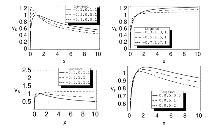
Figure 2: Normalized circular velocity $v_{s}\equiv\frac{v_{c}(x)}{v_{c}(1)}$ for different combinations of the parameters $(\alpha,\beta,x_{0})$. Starting on the top, in the panel on the left we consider model with finite mass ($\alpha+\beta=0$) and on the right models with flat curves ($\alpha+\beta=1$). In the bottom, on the left we fix $\alpha$ and change $\beta=0.5,1.0,1.5$ and on the right $\alpha=0$, $\beta=0.5$ and we change $x_{0}=0.5,1,2$.

4.1 Gravitational potential

Although not explicitly needed to evaluate the dynamical quantities of interest, it is nonetheless useful to compute the gravitational potential for the model we are considering. For spherical systems, it is (Binney & Tremaine (1987)) :

$$\Phi(r)=-\frac{GM(r)}{r}-4\pi G\int_{r}^{\infty}{\rho(r^{\prime})r^{\prime}dr^{\prime}}$$

that, inserting Eqs.(6) and (10) gives :

$$\Phi(x)=-\frac{G\Upsilon_{0}\ L_{tot}}{a\ x_{0}^{\alpha}}\left[\frac{x^{3+\alpha-\gamma}}{(1+x)^{3-\gamma}}\left(1+\frac{x}{x_{0}}\right)^{\beta}+\frac{{\cal{F}}(x;{\bf p})}{x_{0}}\right]$$ (23)

with ${\bf p}$ the set of parameters $(\alpha,\beta,\gamma,x_{0})$ and  :

$${\cal{F}}(x;{\bf p})\equiv\int_{0}^{\infty}{\xi^{\alpha-\gamma+1}(1+\xi)^{\gamma-4}(1+\xi/x_{0})^{\beta-1}{\cal{P}}(\xi)d\xi}\ .$$ (24)

Note that this expression only holds for models with $\alpha+\beta\leq 1$ and is a complicated combination of hypergeometric and Appell functions. As an example, we report the result for $x_{0}=1$ which is the simplest one :

$${\cal{F}}(x)=\left[\frac{\gamma-3-\alpha}{\alpha+\beta-2}{\cal{F}}_{1}(x)+\frac{(\alpha+\beta)x}{\alpha+\beta-1}{\cal{F}}_{2}(x)\right]x^{\alpha+\beta-2}$$ (25)

having defined :

$${\cal{F}}_{1}(x)\equiv{{}_{2}F_{1}(2-\alpha-\beta,4-\beta-\gamma,3-\alpha-\beta,-1/x)}\ ,$$ (26)

$${\cal{F}}_{2}(x)\equiv{{}_{2}F_{1}(1-\alpha-\beta,4-\beta-\gamma,2-\alpha-\beta,-1/x)}\ ,$$ (27)

with ${{}_{2}F_{1}(a,b,c,y)}$ the hypergeometric function (Gradshteyn & Ryzhik (1980)).

The case $\alpha+\beta=1$ merits some discussion since the function ${\cal{F}}$ turns out to be constant. Since the gravitational potential is defined up to an arbitrary additive constant, we may choose this constant in such a way that $\Phi(x)$ for this class of models simplifies to $-GM(x)/x$ which is the well known Keplerian potential of a spherical system with finite total mass.

Finally, we study the asymptotic trends. For $x\to\infty$, $\phi\propto x^{-1+\alpha+\beta}$, thus in order to have a plausible gravitational potential, the models with $\alpha+\beta>1$ are ruled out, so that we conclude that the only physical models are those with

$$\alpha+\beta-1\leq 0\rightarrow\alpha\leq 1-\beta.$$ (28)

4.2 Circular velocity

For a spherically symmetric mass distribution the circular velocity is simply given by

$$v_{c}=\sqrt{\frac{GM(r)}{r}}$$ (29)

which, in our case, becomes :

$$v_{c}(x)=\sqrt{\frac{G\Upsilon_{0}\ L_{tot}}{a\ x_{0}^{\alpha}}\ x^{2+\alpha-\gamma}\ (1+x)^{\gamma-3}\ (1+x/x_{0})^{\beta}}\ .$$ (30)

It is interesting to look at the asymptotic trends :

$$v_{c}^{2}(x)\propto\left\{\begin{array}[]{ll}x^{2+\alpha-\gamma}&{\rm for}\ \ \ x<<1\\ \nobreak\leavevmode&\nobreak\leavevmode\\ x^{\alpha+\beta-1}&{\rm for}\ \ \ x>>1\\ \end{array}\right.\ .$$ (31)

First, we note that $v_{c}$ must vanish at the centre so that we get the condition :

$$2+\alpha-\gamma>0\rightarrow\alpha>\gamma-2$$ (32)

that is more stringent than Eq.(7). We consider as physically motivated those models having an asymptotically flat or decreasing rotation curve. Thus, using Eq. (31), we obtain the constraint in Eq. (28).

In particular, models with $\alpha+\beta=0$ presents a keplerian falloff of the rotation curve consistent with the finite total mass, while $v_{c}$ is asymptotically flat when $\alpha+\beta=1$ with :

$$v_{c}(\infty,\alpha+\beta=1)=\sqrt{\frac{G\Upsilon_{0}\ L_{tot}}{ax_{0}}}\ .$$ (33)

The qualitative dependence of $v_{c}$ on the parameters $(\alpha,\beta,x_{0})$ may be derived by Fig. 2 where we plot the scaled circular velocity $v_{s}\equiv v_{c}(x)/v_{c}(x=1)$ for some representative choices of the parameters $(\alpha,\beta,x_{0})$ and setting $\gamma=1$. In the top left panel, we present models having finite total mass (i.e., with $\alpha+\beta=0$) thus showing a keplerian falloff of the rotation curve. The top right panel, instead, refers to models with asymptotically flat rotation curve that is with $\alpha+\beta-1=0$ corresponding to a $M/L$ ratio that is still increasing beyond the visible edge of the galaxy as in presence of a dark matter halo. In both cases, for a given $x$, $v_{c}$ is a decreasing or increasing function of $\beta$ depending on $x$ being larger or lower than 1 respectively. The situation is reversed when considering the dependence on $\alpha$ with the higher values of $\alpha$ leading to larger (smaller) circular velocities in the regime $x>1$ ($x<1$). The role of $\beta$ is further investigated in the bottom left panel where we hold $\alpha$ fixed and change $\beta$ showing that this slope parameter determines the transition from asymptotically decreasing to asymptotically flat rotation curves. In particular, models with flat rotation curves rotate faster than those with a keplerian falloff. Finally, in the bottom right panel, we investigate the dependence on the scaling radius $x_{0}$ finding out that the larger is $x_{0}$, the lower is $v_{c}(x)$. It is worth noting that the wide variety of cases is an evidence of the extreme versatility of the adopted parametrization even if this originates degeneracies among the parameters $(\alpha,\beta,x_{0})$ that may not be disentangled with observations of the rotation curve only.

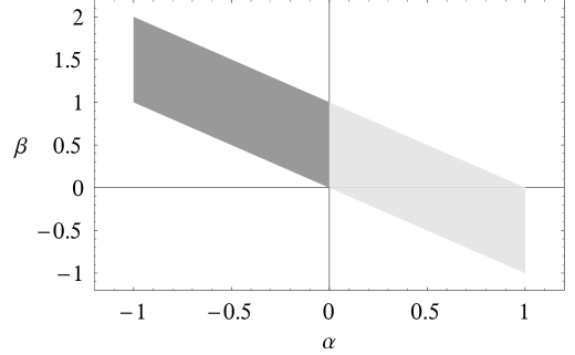
Figure 3: Constraints on model parameters $\alpha$ and $\beta$ for $\gamma=1$. The selected region is allowed by a theoretical analysis on the model and its main related quantities (mass, mass density, surface mass density, gravitational potential and circular velocity). The parameters $\alpha$ and $\gamma$ are crucial in this analysis, in particular to determine the low radii trend of the surface mass density. In the limit $r\rightarrow 0$, the darker region corresponds to diverging (‘cuspy’) $\Sigma$, while the lighter one individuates models with flat (‘cored’) $\Sigma$.

Combining all the constraints obtained insofar on model parameters, we end up with the following range for $\alpha$ :

$$\max{(\gamma-2,-\beta)}\leq\alpha\leq\min{(\gamma,1-\beta)}\$$ (34)

which we have graphically summarized in Fig. 3 for models with $\gamma=1$.

4.3 Velocity dispersion

While the circular velocity is related to the ordered motions in the galactic plane, the velocity dispersion takes into account disordered motions and thus is the main quantity to describe dynamics of non rotating systems like elliptical galaxies. Assuming an isotropic velocity dispersion tensor, the solution of the Jeans equation gives the following general formula (Binney & Tremaine (1987)) :

$$\sigma^{2}(r)=\frac{1}{j(r)}\int_{r}^{\infty}{j(r^{\prime})\frac{GM(r^{\prime})}{r^{\prime 2}}dr^{\prime}}$$ (35)

that, applied to our particular case, reduces to :

$$\sigma^{2}(x)=\frac{G\Upsilon_{0}\ L_{tot}}{a\ x_{0}^{\alpha}}{\times}\frac{I_{\sigma}(x,{\bf p})}{x^{\alpha-\gamma}\ (1+x)^{\gamma-4}(1+x/x_{0})^{\beta-1}{\cal{P}}(x)}$$ (36)

with :

$$I_{\sigma}\equiv\int_{x}^{\infty}{\xi^{1+2(\alpha-\gamma)}(1+\xi)^{2\gamma-7}(1+\xi/x_{0})^{2\beta-1}{\cal{P}}(\xi)d\xi}\ .$$ (37)

This integral is only defined for $\alpha+\beta<2$ which is not a problem given that $\alpha$ nd $\beta$ ranges in the interval defined by Eq.(34). The general analytical expression is again a complicated combination of hypergeometric and Appell functions so that a numerical integration turns out to be easier to handle in the applications. As an example, we only report the case with $x_{0}=1$ that is :

$$I_{\sigma}(x)=\frac{x^{2(\alpha+\beta)-5}}{2(\alpha+\beta-2)\left[2(\alpha+\beta)-5\right]}{\times}$$

$$\ \ \ \ \ \ \ \ \left\{\ 2(2-\alpha-\beta)(3+\alpha-\gamma)\ {\cal{I}}_{1}\ +\right.$$

$$\ \ \ \ \ \ \ \ \left.\left[\ \alpha(2\alpha+4\beta-5)+\beta(2\beta-5)\right]\ x\ {\cal{I}}_{2}\ \right\}$$ (38)

where we have set :

$${\cal{I}}_{1}\equiv{{}_{2}F_{1}(5-2\alpha-2\beta,7-2\beta-2\gamma,6-2\alpha-2\beta,-1/x)}\ ,$$ (39)

$${\cal{I}}_{2}\equiv{{}_{2}F_{1}(4-2\alpha-2\beta,7-2\beta-2\gamma,5-2\alpha-2\beta,-1/x)}\ .$$ (40)

A wide variety of cases is obtained varying the parameters $(\alpha,\beta,x_{0})$. Note, however, that what is indeed observed is not the velocity dispersion $\sigma(x)$, but rather its luminosity weighted projection along the line of sight that we will compute later.

4.3.1 Effects of anisotropy

Eq.(35) only holds under the hypothesis that the velocity dispersion is the same along the three axes of the coordinate system. In the case of a spherically symmetric system, the relation $\sigma_{\theta}=\sigma_{\phi}=\sigma_{t}$ holds, where $\sigma_{\theta}$, $\sigma_{\phi}$ and $\sigma_{t}$ are respectively the polar, azimuthal and tangential velocity dispersion and we can define the anisotropy parameter:

Figure 4: $\Delta\sigma_{s}$ as a function of $\beta_{\sigma}$ for $x=0.1$ (thin dashed), $x=0.5$ (thick dashed), $x=2$ (thin solid) and $x=10$ (thick solid). The model parameters are set as $(\alpha,\beta,\gamma,x_{0})=(-0.5,1.0,1.0,1.0)$.

$$\beta_{\sigma}(r)\equiv 1-\frac{\sigma_{t}^{2}}{\sigma_{r}^{2}},$$ (41)

with $\sigma_{r}$ the radial velocity dispersion; isotropy in the velocity space means $\beta_{\sigma}=0$ (i.e., when $\sigma_{r}=\sigma_{t}$). In the general case, Eq.(35) becomes :

$$\sigma^{2}(r)=\frac{1}{\eta(r)j(r)}\int_{r}^{\infty}{\eta(r^{\prime})j(r^{\prime})\frac{GM(r^{\prime})}{r^{\prime 2}}dr^{\prime}},$$ (42)

where $\eta(r)$ is obtained by solving :

$$\frac{d\log\eta}{d\log r}=2\beta_{\sigma}(r).$$ (43)

To quantify the effect of the anisotropy, we first consider the simplest model $\beta_{\sigma}(r)=const$ and introduce the anisotropy to isotropy ratio parameter $\Delta\sigma_{s}=100\times[\sigma_{s}(x,\beta_{\sigma})/\sigma_{s}(x,0)-1]$, defined as a function of scaled velocity dispersions . In Fig. 4 we plot $\Delta\sigma_{s}$ as a function of $\beta_{\sigma}$ for different values of the dimensionless radius $x$. It turns out that a constant anisotropy significantly alters the velocity dispersion profile, with positive values increasing the velocity dispersion at low and high radii. The amount of the relative variation depends on $x$ and the model parameters $(\alpha,\beta,\gamma,x_{0})$.

Figure 5: $\Delta\sigma_{s}$ as a function of $\mu_{OM}$. The values of $x$, the line coding and the model parameters are the same as in Fig. 4.

A constant anisotropy, although simple and widely used, is not a realistic assumption. More realistic results are obtained considering the Osipkov - Merrit parametrization (Osipkov (1979); Merritt (1985)) :

$$\beta_{\sigma}(r)=\frac{r^{2}}{r^{2}+r^{2}_{OM}}$$ (44)

with $r_{OM}$ the anisotropy radius. Isotropic models are recovered in the limit $r_{OM}\to\infty$. In such a case we can extend the definition of anisotropy to isotropy ratio parameter as $\Delta\sigma_{s}=100\times[\sigma_{s}(x,x_{OM})/\sigma_{s}(x,\infty)-1]$, where $x_{OM}\equiv r_{OM}/a$. In Fig. 5 we plot $\Delta\sigma_{s}$ as a function of $\mu_{OM}\equiv\frac{1}{x_{OM}}$. Although the results are more complicated, it is nevertheless clear that also in this case the anisotropy introduces large changes in the velocity dispersion. $\Delta\sigma_{s}$ converges to $0$ for high $x_{OM}$ (low $\mu_{OM}$) and assumes saturated and very high values for low $x_{OM}$ (high $\mu_{OM}$).

4.3.2 Projected velocity dispersion

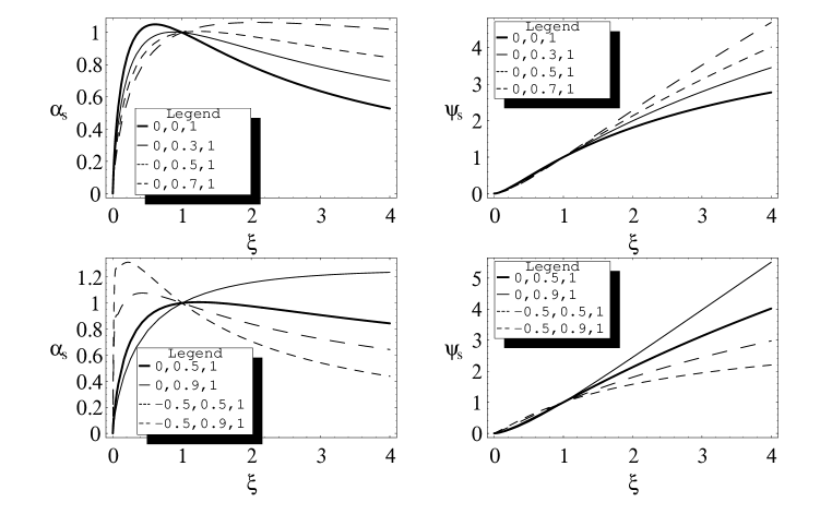
Figure 6: Normalized deflection angle $\alpha_{s}$ (left) and lensing potential $\psi_{s}$ (right) as function of $\xi$. The model parameters $(\alpha,\beta,x_{0})$ are set as in the inset of each panel, while $\gamma=1$ is used for the luminosity profile.

The velocity dispersion defined by Eq.(35) is not directly measurable. Indeed, when comparing to observations, we have to take into account some effects. First, the line of sight does not coincide with the radial direction so that we measure only the projection of the velocity dispersion along the line of sight. Moreover, all the galaxy elements contribute to the measured $\sigma$, but the more luminous is the element, the larger will be its contribution to the observed quantity. As such, we have first to define the velocity dispersion projected along the line of sight and luminosity weighted. Denoting by $\sigma_{los}$ this quantity, it is (Binney & Tremaine (1987)) :

$$\sigma_{los}^{2}=\frac{2}{I(R)}\int_{R}^{\infty}j(r)\frac{GM(r)\sqrt{r^{2}-R^{2}}}{r^{2}}dr$$ (45)

with $I(R)$ the luminosity intensity.

As a second step, we have to take into account the seeing that makes the intrinsic intensity differs from the observed one. We therefore define the seeing corrected velocity dispersion as :

$$\sigma_{seeing}^{2}(R)=\frac{\int d^{2}R^{\prime}P(R-R^{\prime})I(R^{\prime})\sigma_{p}^{2}(R^{\prime})}{\int d^{2}R^{\prime}P(R-R^{\prime})I(R^{\prime})},$$ (46)

where $P(R-R^{\prime})$ is the point spread function taking into accont both the atmospheric and the instrument seeing. Finally, we have to consider the effect of the spatial binning and the finite width of the slit used to make the measurements. Therefore, the measured quantity reads :

$$\sigma_{bin}^{2}=\frac{\int_{A}{dA^{\prime}I_{s}(R^{\prime})\sigma^{2}_{seeing}(R^{\prime})}}{\int_{A}{dA^{\prime}I_{s}(R^{\prime})}},$$ (47)

where $A$ is the area of the slit and $I_{s}$ is the seeing corrected intensity. We do not investigate these observational effects since they are strictly related to the observational setup. We, however, stress the need to carefully take into account these corrective terms in order to not introduce systematic errors when comparing the model to the data.

5 Gravitational lensing

Considered at its early beginning a little more than a scientific curiosity, gravitational lensing has now given rise to what may be referred to as lensing astronomy. Being directly dependent on the mass rather than the light distribution, gravitational lensing has turn out to be an invaluable tool to investigate the total density profile in early type galaxies at intermediate and high redshift. The lensing observable quantities (such as the position of the images and their flux ratios) in multiply imaged sources (quasars or galaxies) make it possible to constrain the mass profile. Combining lensing reconstruction with a measurement of the velocity dispersion helps breaking degeneracies inherent in lens modeling thus shedding a powerful light on their dark matter content (Treu & Koopmans 2002a ; Treu & Koopmans (2004)). Understanding the mass distribution of the lens plays a key role also in the determination of the Hubble constant $H_{0}$ through the time delay method (Refsdal (1964)). In particular, Kochanek (2002) has shown that the predicted delay between two images, and hence the derived value of $H_{0}$, is primarily governed by the average surface mass density in the annulus defined by their radial distances from the lens center with a small correction taking into account the slope of the profile in this annulus. A careful determination of mass profile is therefore mandatory to get a reliable estimate of $H_{0}$ and hence of the distance scale. Lens modeling plays a vital role also in cosmological applications of gravitational lensing. Since early - type galaxies are expected to represent at least 80$\%$ of lenses (Turner et al. (1984); Fukugita & Turner (1991)), a correct description of their luminous and dark component is an essential ingredient in every attempt to constrain cosmological parameters through statistics of lens systems.

Motivated by these considerations, we complement our presentation of our new phenomenological model by a detailed investigation of its lensing properties.

5.1 Deflection angle and lensing potential

For a spherically symmetric model, the deflection angle $\hat{\alpha}$ may be easily computed as :

$$\hat{\alpha}(\xi)=\frac{2a}{\xi}\int_{0}^{\xi}{\kappa(u)udu}=\hat{\alpha}_{1}{\times}\alpha_{s}(\xi;{\bf p})$$ (48)

where the normalized deflection angle $\alpha_{s}$ depends on the dimensionless radius $\xi=R/a$ and the model parameters ${\bf p}=(\alpha,\beta,\gamma,x_{0})$, while $\hat{\alpha}_{1}$ is the value of the deflection angle for $\xi=1$. The normalized surface mass density $\kappa$ is defined as the ratio $\Sigma/\Sigma_{crit}$ between the surface mass density $\Sigma$ and the critical surface density $\Sigma_{crit}\equiv c^{2}D_{s}/(4\pi GD_{d}D_{ds})$ with $D_{s}$, $D_{d}$ and $D_{ds}$ the source, lens and lens - source angular diameter distances.

Figure 7: Left. Time delay function $\Delta t$ (measured in days) as a function of the radial distance from the centre (measured in ${\rm arcsec}$). Note that negative values of $r$ corresponds to radial distances after a rotation of $\pi$ radians. Model parameters are set as $(\alpha,\Upsilon_{0},x_{0})=(-0.3,5.0,1.0)$ and three values of $\beta$ are considered, namely $\beta=0.8$ (solid), $\beta=1.0$ (long dashed), $\beta=1.2$ (short dashed). For the luminosity profile, we set $\gamma=1$, while the source position is $r_{s}=0.3\ {\rm arcsec}$. The extremals of the function corresponds to the images. Right. $\Delta t$ as function of $\beta$ for three values of $\alpha$, namely $\alpha=-0.3$ (solid), $\alpha=-0.5$ (long dashed) and $\alpha=-0.7$ (short dashed). The remaining model parameters are set as before, while we move the source at $r_{s}=0.1\ {\rm arcsec}$ and evaluate $\Delta t$ at $r=1\ {\rm arcsec}$.

Although quite complicated analytical expression are possible for $\alpha_{s}$, we prefer to not report them here and discuss the results looking at the left panels in Fig. 6. In particular, in the top left panel, we consider models with an inner core ($\alpha=0$) and find out that the larger is $\beta$, the higher (the lower) is the deflection angle for $\xi>1$ ($\xi<1$). Note that, in the outer regions, $\alpha_{s}(\xi)$ is always larger than what is predicted by a constant $M/L$ model. In the bottom left panel, we show the effect of changing $\alpha$ while holding $\beta$ fixed. It turns out that increasing $\alpha$ strongly lowers the deflection angle in the outer regions ($\xi>1$) with only a minor effect for $\xi<1$. These trends are consistent with the asymtptotic scalings $\alpha_{s}\propto\xi^{\alpha-\gamma+2}$ for $\xi<<1$ and $\alpha_{s}\propto\xi^{\alpha+\beta-1}$ for $\xi>>1$. Note that, as expected, for models with finite total mass $(\alpha+\beta=0)$, we get $\alpha_{s}\propto 1/\xi$ as for a point mass lens. Finally, we note that $\alpha_{s}$ is an increasing function of $x_{0}$ which can be explained by noting that the larger is $x_{0}$, the more the model is concentrated and hence more mass is within a circle with radius $\xi$ and hence the larger is the deflection angle.

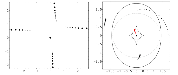
Figure 8: Image configurations for different values of the parameters : the dimension of the spot changes varying the parameters. Left. We set the source position $r_{s}=0.1^{\prime\prime}$ and let $\beta$ increasing (the higher is $\beta$, the greater is the spot). Right. Here $\beta$ is fixed at 1 and $r_{s}$ changes. The bold continue line is the critical curve and the corresponding caustic is the astroid (dashed bold curve at center); the internal lighter continue ellipse is the radial critical curve and the corresponding caustic is the dashed lighter ellipse. In both the panel we set $\alpha=-0.3$, $\Upsilon_{0}=5$, $\theta_{s}=20^{\circ}$, $\gamma_{s}=0.15$ and $\theta_{\gamma_{s}}=180^{\circ}$.

The spherical symmetry of the model makes it possible to straightforwardly compute the lensing potential integrating the deflection angle thus obtaining :

$$\psi=a\int{\hat{\alpha}(\xi)d\xi}=\psi_{1}{\times}\psi_{s}(\xi;{\bf p})$$ (49)

with $\psi_{s}$ the scaled potential and $\psi_{1}=\psi(\xi=1)$. The complete expression of $\psi_{s}$ is too cumbersome and will be not reported here. However, we plot $\psi_{s}$ as a function of $\xi$ for some representative models in the right panels of Fig. 6 showing that $\psi_{s}$ is an increasing function of $\beta$. For $\xi\to 0$, $\psi_{s}\propto\xi^{\alpha-\gamma+3}$, while $\psi_{s}\propto\xi^{\alpha+\beta}$ as $\xi\to\infty$. Note that both these trends should be derived directly from those of $\alpha_{s}$ given how $\alpha_{s}$ and $\psi_{s}$ are related.

The deflection potential is an essential ingredient to write down the time delay function and hence estimate the time delay between the images in the multiply imaged quasars. Adopting polar coordinates $(R,\theta)$ in the lens plane with $\theta$ measured counterclockwise from North, it is :

$$\Delta t=h^{-1}\tau_{100}\ a^{2}\bigg{[}\frac{1}{2}\xi^{2}-\xi\ \xi_{s}\cos(\theta-\theta_{s})+\frac{1}{2}\xi_{s}^{2}-\psi(\xi,\theta)\bigg{]},$$ (50)

where $(\xi,\theta)$ and $(\xi_{s},\theta_{s})$ are the images and source positions, $h$ the dimensionless Hubble constant and $\tau_{100}=(1+z_{d})/c{\times}D_{d}D_{s}/D_{ds}$ with $z_{d}$ the lens redshift. According to the Fermat principle, the images form at the extrema of the time delay function so that the lens equations are :

$$\xi-\xi_{s}\cos(\theta-\theta_{s})=\frac{\hat{\alpha}(\xi)}{a},$$ (51)

$$\xi_{s}\sin(\theta-\theta_{s})=0\ .$$ (52)

Eq.(52) reduces to an identity for $\xi_{s}=0$, i.e. the lens and the source are perfectly aligned. In this case, the image is the well known Einstein ring with radius obtained by solving Eq.(51) for $\xi_{s}=0$. Alternatively, Eq.(52) is solved by $\theta=\theta_{s}+n\pi$ with $n=0,1$. Inserting these values in Eq.(51) and solving with respect to $\xi$, we get three images. Two of them are disposed symmetrically with respect to the lens centre, while the third one lies very close to the centre (with $\xi\simeq 0$) and turns out to be unobservable.

A quantitative investigation of the time delay function is shown in Fig. 7. In the left panel, we plot $\Delta t$ as function of the radial distance $r$ for different values of the model parameters. Note that, as expected, the function $\Delta t(r)$ has a maximum and two minimum thus meaning that three images are formed. In the right panels, $r$ is held fixed and we plot $\Delta t$ as function of $\beta$ for different values of $\alpha$. An image forming at $r$ will be more and more delayed as $\alpha$ and $\beta$ get higher. A detailed analysis of the dependence of $\Delta t$ on the model parameters is quite complicate because of the many parameters involved (including the source position) so that will be not performed here.

5.2 Lens ellipticity and contribution of the shear

Real galaxies are hardly spherically symmetric. An easy way to take into account the ellipticity of the lens should be to insert it by hand in the lensing potential replacing the cylindrical dimensionless radius $\xi$ with its elliptical counterpart $\tilde{m}=\sqrt{\xi_{1}^{2}+\xi_{2}^{2}/q^{2}}$ with $q$ the axial ratio. A still simpler approach is to add an external shear to the lensing potential since it has been shown that an elliptical potential $\psi(\tilde{m}^{2})$ with an on axis shear $\gamma_{s}$ and axial ratio $q$ produce the same image configuration as a pure elliptical potential with an axial ratio $q^{\prime}=q[(1-\gamma_{s})/(1+\gamma_{s})]^{1/2}$ and no shear (Witt (1996)). Moreover, an external shear could also mimic the effect of tidal perturbations from nearby galaxies or departures from a smooth distribution because of substructures in the primary lens. Motivated by these considerations, we add the shear term :

$$\psi_{\gamma_{s}}=-\frac{1}{2}\gamma_{s}a^{2}\xi^{2}\cos{2(\theta-\theta_{\gamma_{s}})}$$ (53)

to the lensing potential $\psi$ being $(\gamma_{s},\theta_{\gamma_{s}})$ the shear strength and direction.

The main effect of the shear is to alter the shape of the critical curves, defined as the loci in the lens plane where the magnification formally diverges. In particular, not considering the radial critical curve, the higher is $\gamma_{s}$, the larger is the deformation of the tangential critical curve. In the case of no shear, this curve coincides with the Einstein ring, while, for $\gamma_{s}\neq 0$, we have to distinguish two closed curve: the first one elongated along the direction of the shear itself (the critical curve) and the other one in perpendicular direction (the Einstein ring). Moreover, the larger is $\gamma_{s}$, the lower will be the axial ratio $b/a$ between the shortest and the longest axis of these ellipses.

5.3 Image formation

As quoted above, the axisymmetric lens can produce only 2 images with in addition a central (observationally not visible) one. When we distort the lensing isopotential contours by adding the shear term, the shape of tangential critical curves changes and the point - like caustic unfolds generating four cusps (Schneider, Ehlers & Falco (1992)). It is interesting to discuss the formation of the images as a function of some of the model parameters for the case with the shear term included.

In Fig. 8, we plot the image configuration for some values of the parameters and changing $\beta$ or $r_{s}$. We can see how the model can generate 3 or 5 images (2 or 4 plus a central image). In the left panel, we fix the source position and change the values of $\beta$ finding that the radial coordinate of the image increases with $\beta$. The right panel shows, for a fixed $\beta$, how the number and the position of the images change with the source position $r_{s}$. Increasing $r_{s}$ two of the images approach each other in direction of the tangential critical curve, until the source exits the region delimited by the tangential caustic curve (the central astroid) when the two images merge and the system passes from a 5 - images to a 3 - images configuration. The other two curves in figure represents the radial critical curve and the corresponding caustic.

The number of images needs a brief remark. The odd-number theorem predicts that lenses with a smooth and not singular surface mass density $\kappa(R)$ which decreases faster than $R^{-1}$ as $|R|\to 0$ necessarily forms an odd number of images. For models with $\kappa$ diverging for $R\to 0$, we can use a generalized version of the previous theorem given by Evans & Wilkinson (1998). These authors consider models with an inner cusp and $\kappa\propto R^{-n}$ (e.g., NFW models above described) and distinguish three different behaviours (see Ref. above for major details)

1. if $0<n<1$ (weak density cusp), then we observe an odd number of images

2. if $1<n<2$ (strong density cusp), then we observe an even number of images

3. if $n=1$ (isothermal density cusp), then we can observe both an odd or even number of images

Our model can predict an asymptotically decreasing (flat) $\kappa$ for $\gamma-2<\alpha<\gamma-1$ ($\gamma-1<\alpha<\gamma$). When $\gamma-2<\alpha<\gamma-1$ is $n=-(\alpha-\gamma+1)$ and it is simple to verify that these models belong to the weak density cusp class, with $0<n<1$, thus an odd number of images always exist as observed in Fig. 8 for all the values of $\gamma$. In addition, when $\kappa$ is cored (for instance, if $\gamma-1<\alpha<\gamma$), then the original odd-number theorem holds and predicts also in this case an odd number of images. Thus, our model cannot reproduce strong cusp, predicting for all the possible combinations of the lens parameters an odd number of images and the formation of both radial and tangential critical curves (the first one not observed in the case of strong cusp models). Nearly all the observed lenses present two or four images, thus a discordance appears. However, observations and theoretical predictions can be reconciled if the central image is very close to the lens and highly demagnified by the high central surface density, making this image difficult to detect. Actually, central images were observed in the 2-image lens PMN J1632-0033 (Winn et al. 2003, 2004), therefore the existence of these events can allow to constrain the lens model and particularly the inner slope of the mass density.

5.4 Comparison with commonly used lens models

Having investigated in detail the lensing properties of our phenomenological model, it is worth comparing it with some of the most used models in literature.

As a quite general and simple class of models, we consider the power law lensing potential :

$$\psi(R,\theta)=R^{\nu}F(\theta,q,\theta_{q})$$ (54)

where $0<\nu<2$ is the slope of the radial profile and $F(\theta,q,\theta_{q})$ the angular shape function with $(q,\theta_{q})$ the axial ratio and the orientation of the isopotential contours. Eq.(54) represents a generalization of the the pseudo - isothermal elliptical potentials (Kovner (1987); Kassiola & Kovner (1995)) that have been designed to be as similar as possible to the pseudo - isothermal mass distribution models (Blandford & Kochanek (1987); Kassiola & Kovner (1995)). Given their easy manageability, they have been widely used in literature. For semianalytical and/or numerical treatments in modeling lensed quasars see, e.g., Cardone et al. (2001, 2002), Tortora et al. (2004). In addition, considering that $\kappa\propto R^{\nu-2}$ and following the previous Sec., power law with $0<\nu<1$ ($1<\nu<2$) have strong (weak) cusp.

It is worth stressing that the models defined by Eq.(54) are characterized by a constant radial slope of the lensing potential. Obviously, this is not the case for our phenomenological model. Nevertheless, we can match the two models in the inner regions by setting $\alpha-\gamma+3=\nu$. In particular, for $\gamma=1$ and $\xi\rightarrow 0$, our model reproduces the pseudo - isothermal trend for $\alpha\in[-1,0]$ thus excluding the region $(0,1]$, since for these values of $\alpha$ is $\nu>2$ and the pseudo - isothermal models generate a non physical surface mass density. It is possible to match the outer slope imposing $\alpha+\beta=\nu$: also in this case the matching is not complete since when $\alpha+\beta>1$ our models are not defined, on the contrary the models in Eq. (54) holds also for $\nu\in(1,2]$.

6 Conclusions

The rotation curves of spiral galaxies have been the first observational cornerstone of the dark matter theory. The nature and the distribution of this unseen component of galaxies are still obscure, but more and more evidences have been accumulated in favour of its ubiquitous presence. Nonetheless, this picture is far to be free of its own problems since recent observations of line of sight velocity profile of elliptical galaxies have furnished contrasting evidences favoring or disfavoring the presence of significant amounts of dark matter in the outer regions of these systems. In an attempt to face this problem we have employed here a phenomenological approach assuming a double power law expression for the global $M/L$ ratio as $\Upsilon(r)=\Upsilon_{0}(r/r_{0})^{\alpha}(1+r/r_{0})^{\beta}$. This simple parametrization reduces to constant $M/L$ models for $(\alpha,\beta)=(0,0)$, while gives an asymptotically increasing $M/L$ ratio for $\alpha+\beta\geq 0$ as in models with dominating dark matter component. Adopting spherical symmetry and a versatile expression for the luminosity density $j(r)$, it is possible to build a wide class of (effective) galaxy models starting from the mass profile $M(r)=\Upsilon(r)L(r)$. Varying the model parameters $(\alpha,\beta)$ in the range determined by some physical considerations makes it possible to mimic a wide range of models having finite $(\alpha+\beta=0)$ or formally infinite $(\alpha+\beta>0)$ total mass, cuspy $(\alpha-\gamma<0)$ or cored $(\alpha-\gamma=0)$ density profiles, asymptotically flat $(\alpha+\beta-1=0)$ or decreasing $(\alpha+\beta-1<0)$ rotation curve, cuspy $(\gamma-2<\alpha<\gamma-1)$ or cored $(\gamma-1<\alpha<\gamma)$ surface mass density.

The main advantage of our parametrization of the $M/L$ model is therefore the possibility to reproduce a wide phenomenology resorting to a simple analytical expression and relying on phenomenological considerations only thus avoiding any theoretical prejudice or systematic errors related to convergence problems in numerical N - body simulations of structure formation. As a preliminary and mandatory step, to allow a future comparison between theoretically predicted and observed properties of early type galaxies, we have here derived the main dynamical and lensing quantities of the model giving whenever possible analytical expressions or illustrative plots. We have payed a particular attention to the asymptotic trends in the inner and outer regions since both these regimes are mostly probed by different kind of observations. On the one hand, measurement of the velocity dispersion profiles hardly extends to radii larger than the effective radius $R_{e}$ and, indeed, only the central velocity dispersion is often at disposal. Such a mass tracer therefore mainly probes the inner region of the system so that knowing how our model fares for $x<<1$ helps in comparing with this kind of data. In order to probe larger radii, one may resort to multiply imaged lensed quasars. First, the images typically form at $r\sim(1\,-\,2)R_{e}$ so that a larger region is probed. Moreover, the lensing potential and the flux ratios also depend on the derivatives of the mass profile thus allowing to probe indirectly also outermost regions.

We can individuate two main implications. Firstly, we have seen how the the full mass density profile and derived DM profile depend on $\gamma$ and therefore on the fitted luminous profile. Therefore, the presence of the baryons influences dark matter profile, since the parameter $\gamma$ that specifies the inner slope of the luminous profile enters in the expression of halo profile derived from our model. Secondly, we have compared our model with the more common generalized NFW profile: the asymptotic trends has been compared and we are able with suitable choices of $\alpha$ and $\beta$ to recover the behaviour of gNFW model. The value of the inner trend of mass profile has generated a long debate in literature. The simulations seems to indicate an inner trend that scales like $r^{-\delta}$ with $\delta\geq 1$ (the so called cusped models). On the contrary, many results from observational analysis, by rotation curves of low surface brightness, dwarf galaxies and spiral galaxies, dynamical studies of elliptical galaxies and gravitational lensing (McGaugh & de Blok (1998); Binney & Evans (2001); Borriello & Salucci (2001); de Blok et al. (2001); Treu & Koopmans 2002b ; Borriello et al. (2003)) suggested the presence of internal core with $\delta<1$ (cored models). This contradiction generates the so called cusp/core problem. Our model can reproduce both cuspy models with $\delta\geq 1$ and cored ones with $\delta<1$. In details, $\alpha<0$ recovers the first models, i.e. the results from simulations and $\alpha\geq 0$ the seconde one, those from results of observations. Being able to reproduce all these different behaviours, our phenomenological model offers the perspective to homogenously analyze the observations and give an answer to the cusp/core problem.

On a theoretical side, our approach could be further ameliorated. A key ingredient in our modeling is the luminosity density $j(r)$ which we have assumed to be described by the class of Dehnen models. Although this gives a quite general expression able to reproduce well the observed surface brightness profile, the ideal route to follow should be to deproject an empirical function obtained by a direct fit to the photometric data. However, this approach should be repeated for each single galaxy and thus does not allow to investigate general properties. An intermediate possibility could be to use the deprojection of the Sersic profile as input for the luminosity density and investigate the dynamical and lensing properties of the corresponding model. Moreover, it has been shown that the dynamics of inner regions of elliptical galaxies is better described adding the contribution of the central supermassive black hole (Baes & Dejonghe (2004); Mamon & Lokas 2005a ; Mamon & Lokas 2005b ) so that it is interesting to update our parametrization including this term into the mass profile. Finally, departures from spherical symmetry could also be investigated since real galaxies are likely to be moderately triaxial systems (Franx et al. (1994)).

Contrasting the model with the observations is, of course, the best strategy to both test the viability of our parametrization and constrain its parameters. Given the difficulties in obtaining radial velocity dispersion profile up to large radii, an ideal tool could be represented by lens galaxies. With more than 90 observed multiply imaged quasars, gravitational lensing offers a unique dataset to put severe constraints on the slope parameters $(\alpha,\beta)$ and hence suggest useful hints to solve the problem of dark matter in elliptical galaxies. Moreover, since lens galaxies span a range in redshift from low to intermediate, such an analysis also offers the possibility to investigate whether and how the characteristics of the dark matter content of early type galaxies evolve.

A first qualitative result can be obtained considering the index of the surface mass density defined as ${\rm ind}{\kappa(r)}=d\ln{\kappa}/d\ln{r}$. In order to shape lensing events with their model independent analysis, Williams & Saha (2000) have used as a constraint on the chosen lens model the condition ${\rm ind}{\kappa(r)}\leq-0.5$ for values of $r$ close to the images positions in strongly lensed quasars (see also Tortora et al. (2004)). Such a condition ensures that the image magnification is less than $\sim 2$ which is a quite plausible constraint well satisfied in some real lenses. Considering that typically images forms at $(1\,-\,2)R_{e}$, we have checked that the constraints on ${\rm ind}{\kappa(r)}$ is satisfied by our model for all physically reasonable choices of the slope parameters. Although this does not allow to further constrain $(\alpha,\beta)$, this result suggests that our parametrization of the $M/L$ ratio leads to a model that correctly reproduces this aspect of the observed lensing phenomenology.

A detailed investigation of some interesting cases is outside our aim here and will be presented in a forthcoming paper. Here, we only note that, although the luminous component parameters $(\gamma,a)$ may be set from the analysis of the surface brightness profile, severe degeneracies still exist among the slope parameters $(\alpha,\beta)$ and the scaling quantities $(\Upsilon_{0},x_{0})$. As a consequence, it is likely that reliable constraints could be obtained only considering bright quadruply imaged systems so that the errors on the image positions is low and the number of constraints higher. Moreover, it is preferable to limit the attention to isolated lens galaxies in order to avoid to introduce further unknown parameters to describe the lens environment. Finally, it is highly desirable to have a measurement of the central velocity dispersion in order to break some of the degeneracies inherent in lens modeling with the help of dynamical data (Treu & Koopmans 2002a ; Treu & Koopmans (2004)).

As a final comment, we would like to stress again the need for a phenomenological approach to the problem of dark matter in elliptical galaxies. In order to overcome any theoretical prejudice, one should adopt a procedure that matches a large set of observational constraints with the minimal number of hypotheses. Adding gravitational lensing data to the dynamical one makes it possible to advance our knowledge on the observational side of the problem. Using phenomenological models like the one we have presented here could be the theoretical ingredient best suited to be coupled to the above data to analyze the question of dark matter in early-type galaxies.