New Debris Disks Around Nearby Main Sequence Stars: Impact on The Direct Detection of Planets
Abstract
Using the MIPS instrument on the Spitzer telescope, we have searched for infrared excesses around a sample of 82 stars, mostly F, G, and K main-sequence field stars, along with a small number of nearby M stars. These stars were selected for their suitability for future observations by a variety of planet-finding techniques. These observations provide information on the asteroidal and cometary material orbiting these stars - data that can be correlated with any planets that may eventually be found. We have found significant excess 70 µm emission toward 12 stars. Combined with an earlier study, we find an overall 70 µm excess detection rate of % for mature cool stars. Unlike the trend for planets to be found preferentially toward stars with high metallicity, the incidence of debris disks is uncorrelated with metallicity. By newly identifying 4 of these stars as having weak 24 µm excesses (fluxes 10% above the stellar photosphere), we confirm a trend found in earlier studies wherein a weak 24 µm excess is associated with a strong 70 µm excess. Interestingly, we find no evidence for debris disks around 23 stars cooler than K1, a result that is bolstered by a lack of excess around any of the 38 K1-M6 stars in 2 companion surveys. One motivation for this study is the fact that strong zodiacal emission can make it hard or impossible to detect planets directly with future observatories like the Terrestrial Planet Finder (TPF). The observations reported here exclude a few stars with very high levels of emission, 1,000 times the emission of our zodiacal cloud, from direct planet searches. For the remainder of the sample, we set relatively high limits on dust emission from asteroid belt counterparts.
1 Introduction
A planetary system is characterized by the properties of its parent star, by the number and nature of its gas-giant and rocky planets, by the extent of its Kuiper and asteroid belts, and by the populations of gas and dust orbiting the central star. In the coming decade, astronomers will use a variety of techniques to address all these aspects of neighboring solar systems. Initial results for gas-giant planets are based on ground-based radial velocity searches. Eventually, nearby stars will be the targets of indirect and ultimately direct searches for terrestrial planets with the Space Interferometer Mission (SIM) and the Terrestrial Planet Finder (TPF). The Spitzer telescope is uniquely positioned to characterize the evolution, amount, structure and composition of the dust associated with Kuiper and asteroid belts around many types of stars, including those with and without the gas giant planets now being detected by the radial velocity technique. Guaranteed Time Observer (GTO) studies such as the FGK sample (Beichman et al., 2005b; Bryden et al., 2006a) and the Nearby Stars program (Gautier et al., 2006), plus the FEPS Legacy project (Meyer et al., 2004; Kim et al., 2005), have conducted photometric surveys of about 200 nearby stars at 24 and 70 µm. The photometric survey discussed here uses Spitzer images at 24 and 70 µm to look for debris disks around an additional 82 stars, rounding out existing surveys of the closest stars.
As the Spitzer programs are completed, we will be able to carry out statistical investigations of the debris disk phenomenon in terms of the age, metallicity, and spectral type of parent stars. In particular, by nearly doubling the size of the existing sample of stars (relative to the on-going GTO/Legacy programs) we can hope to identify and improve the statistics of types of excess that appear to be rare based on existing IRAS or ISO observations, e.g. hot dust, extremely large disk to star luminosity ratios () around mature stars (Fajardo-Acosta et al., 2000; Habing et al., 2001; Spangler et al., 2001), or low mass stars. The incidence of excesses at the IRAS/ISO sensitivity level is about 15% (Backman & Paresce, 1993; Bryden et al., 2006a) so that a total Spitzer sample of 250-300 stars can hope to identify over 50 stars with excesses suitable for future study. Stars with hot excesses (peak wavelength 24 µm) are considerably rarer, 2-3% (Fajardo-Acosta et al., 2000; Laureijs et al., 2002; Beichman et al., 2006), so that a survey of a large number of stars is needed to generate a statistically meaningful sample.
As the statistics of planets build up, we will be able to correlate the properties of debris disks (total mass, physical configuration, composition) with properties of number, location, and mass of planets. Much lower dust masses can be detected with Spitzer than was previously possible, particularly for solar-type and cooler stars. Beichman et al. (2005b) and Bryden et al. (2006a) have shown that with Spitzer instruments, we can reach just a few times the fractional luminosity predicted for our own Kuiper Belt (; Backman & Paresce, 1993; Stern, 1996). Determining how many mature stars like the Sun have Kuiper Belts comparable to our own is an important ingredient in understanding the formation and evolution of solar systems like our own (Levison & Morbidelli, 2003).
Finally the Spitzer data will help us to understand the potential influence of zodiacal emission on the eventual direct detectability of planets. As highlighted in a number of TPF studies, including the Precursor Science Roadmap for TPF (Lawson et al., 2004), the level of exo-zodiacal emission can affect the ability of TPF to detect planets directly, particularly for extreme cases with much greater dust contamination than in the Solar System. A complete census of potential TPF stars will assist in the eventual selection of TPF targets by determining or setting a limit to the amount of exo-zodiacal emission around each star.
This paper focuses on the results of the 24 µm and 70 µm survey using the Multiband Imaging Photometer (MIPS) instrument on Spitzer (MIPS; Rieke et al., 2004). After describing our target selection (§2), we present these MIPS observations in §3. As will be discussed below, a number of sources in this sample appear to be extended. These are highlighted in §3, but are discussed in detail in a separate paper (Bryden et al., 2006b). Follow-up observations of sources with excesses using the IRS spectrometer are just now being completed; these will also be detailed in a later paper. In §4 we discuss how our MIPS flux measurements constrain the dust properties in each system. For the systems identified here as having IR excess, combined with those from Bryden et al. (2006a), §5 attempts to find correlations between the dust emission and system parameters such as stellar metallicity, spectral type, and age. Finally, in 6 we assess the influence of debris disks on the detectability of planets.
2 Stellar Sample
Our sample is based on work carried out by radial velocity search teams (e.g. Marcy et al., 2004) and by the SIM and TPF Science Teams to identify the most suitable targets for the indirect or direct detection of terrestrial-mass planets (1-10 ). One target list consists of the 100 stars in the SIM Tier-1 sample which will be the most intensively observed stars in the two SIM projects dedicated to finding planets around nearby stars (Marcy et al., 2002; Shao et al., 2002). 111The merged, high priority target list for these projects is available at http://astron.berkeley.edu/gmarcy/sim_draft.html. Since the absolute astrometric signal from a planet scales as 3 , the SIM teams are concentrating on the some of the closest, lower mass stars for their deepest surveys for terrestrial planets. Thus, the SIM list includes a number of late K and M stars not included in the other Spitzer samples or in TPF lists.
We also draw from a number of lists prepared by Science Working Groups for the TPF-Coronagraph (TPF-C) and TPF-Interferometer (TPF-I) missions. Although the TPF lists are not definitive given the indeterminate status of the project, the outline of the sample is clear (Beichman et al., 2005c; Traub et al., 2006). We start with F0 - M5 stars of luminosity classes IV or V and refine the list by making a few simple assumptions about the nature of planetary systems and the properties of TPF. Specifically, we 1) exclude stars with binary companions within 100 AU as being inimical to the formation or stable evolution of planetary systems; 2) require that the angular extent of the habitable zone (Kasting et al., 1993); 1 AU for a 1 luminosity star, scaled by the square root of the stellar luminosity) exceed 50 milliarcsec; and 3) impose an outer distance cutoff of 25 pc (although we allowed a few F0-F5 stars at distances as great as 30 pc to bring up their numbers). To enable good measurements with Spitzer we rejected stars with high levels of stellar and/or cirrus confusion based on examination of IRAS maps.
Comparison of potential SIM and TPF targets in cirrus-free sky with the Spitzer Reserved Object Catalog (as of November 2003) showed 81 stars with spectral types ranging from F0 to M3.5, as listed in Table New Debris Disks Around Nearby Main Sequence Stars: Impact on The Direct Detection of Planets. One more star, GL 436, was added through a Director’s Discretionary Time proposal after the discovery of a planet in this system was announced (Butler et al., 2004). Binary companions within the 82 fields of view have also been included as secondary targets; six such companions are identified as bright enough for clear detection in both the 24 and 70 µm images.222The 24 µm image of HD 265866 has what appears to be an equal-brightness binary companion located 40′′ NW of the target primary star. However, there is no visible or near-IR neighboring source. In fact, the second 24 µm source is a chance alignment with a passing asteroid. Software specifically developed for locating asteroids relative to the Spitzer observatory (part of the Horizons package; Giorgini, 2005) identifies this object as asteroid #11847 (“Winckelmann”: H=13.4, a=2.67 AU, e=0.065, i=10.23; Bowell, 1996). The divergent proper motion of HD 48682B, an M0 star 30′′ to the NE of HD 48682, rules out a physical association between the two stars. Thus, HD 48682B is not included in this sample. The true binarity of the other six neighboring sources is verified via their Hipparchos distances and space motion measurements. Angular separations in these systems range from 10′′ to 100′′, with projected orbital separations between 100 and 1000 AU. Data for the companions are listed separately at the end of Tables New Debris Disks Around Nearby Main Sequence Stars: Impact on The Direct Detection of Planets and 2. With their inclusion, our total sample contains 88 stars within 82 targeted fields.
Binned by spectral type, the SIM/TPF sample consists of 37 F stars, 19 G stars, 24 K stars, and 8 M stars. Typical distances range from 10 to 20 pc, closer for M and K stars and farther for earlier spectral types. Figure 1 shows the overall distribution of observed spectral types. Some basic parameters of the sample stars are listed in Table New Debris Disks Around Nearby Main Sequence Stars: Impact on The Direct Detection of Planets, most importantly age and metallicity, which are also shown as histograms in Figures 2 and 3. There is no explicit target selection based on stellar age or metallicity, but known planet-bearing stars have been specifically included in a couple cases. Of this sample, only two stars (GJ 436 and HD 147513) are already known to have planets; most of the other stars with planets are either too faint, lie in cirrus-contaminated regions, or are already observed in other Spitzer programs (e.g. Beichman et al., 2005b).
In this paper we first discuss the 88 primary and secondary stars and then add in the stars observed in Bryden et al. (2006a) to increase the size of the sample for some of statistical discussions.
3 Spitzer Observations
All stars were observed with MIPS at 24 µm and, with one exception (HD 265866), at 70 µm. In order to help pin down their stellar photospheres, four M stars - GJ 908, HD 36395, HD 191849, and HD 265866 - were also observed with the IRAC camera in subarray mode at all four of its wavelengths (3.6, 4.5, 5.8, and 8.0 µm). Seven stars identified as having IR excess were observed with IRS, the Spitzer spectrograph, as follow-up observations, as detailed in a future paper.
3.1 Data Reduction
3.1.1 MIPS Observations
Overall, our data analysis is similar to that previously described in Beichman et al. (2005b) and Bryden et al. (2006a). At 24 µm, images were created from the raw data using the DAT software developed by the MIPS instrument team (Gordon et al., 2005). At 70 µm, images were processed beyond the standard DAT software to correct for time-dependent transients, corrections which can significantly improve the sensitivity of the measurements (Gordon et al., 2004). For both wavelengths, aperture photometry was performed using apertures sizes, background annuli, aperture corrections, and instrument calibration as in Beichman et al. (2005b). We find that the target locations in the 24 µm images are consistent with the telescope pointing accuracy of 1′′ (Werner et al., 2004). As such, we use the 24 µm centroid as the target coordinates for both wavelengths. Special consideration is made for the 6 resolved binaries in our sample. Instead of our standard method of aperture photometry with a surrounding sky annulus, the emission at the two stars’ locations is fit with the instrument’s point spread function (PSF). We find that for binary stars with small angular separations, simultaneously fitting of their overlapping PSFs results in much improved photometric accuracy. The agreement between PSF fitting and aperture photometry (with appropriate aperture correction) for isolated stars is excellent (Gordon et al., 2005). For all of the stars, the MIPS flux and noise measurements are listed in Table 2.
3.1.2 IRAC Observations
The IRAC sub-array images of the four M stars were reduced following the technique described by the FEPS Legacy team (Carpenter et al., 2006). The pixel sizes are corrected for distortion and a pixel-phase correction is made to channel 1. Stellar fluxes are measured within an aperture of 10 pixels (=12′′), with a background annulus from 10 to 20 pixels. The photometric measurements each star at the four IRAC wavelengths are listed in Table 3.
3.2 Photospheric Extrapolations and Limits on 24 µm Excess
To determine whether any of our target stars have an IR excess, we compare the measured photometry against predicted photospheric levels. A detailed description of our stellar atmosphere fitting, as applied to F5-K5 stars, is presented in the appendix of Bryden et al. (2006a). The stars observed here, however, span a greater range of spectral types than previously considered. In particular, our sample contains late K and M type stars with numerous broad molecular features for which the stellar models (Kurucz, 2003) begin to lose their accuracy.
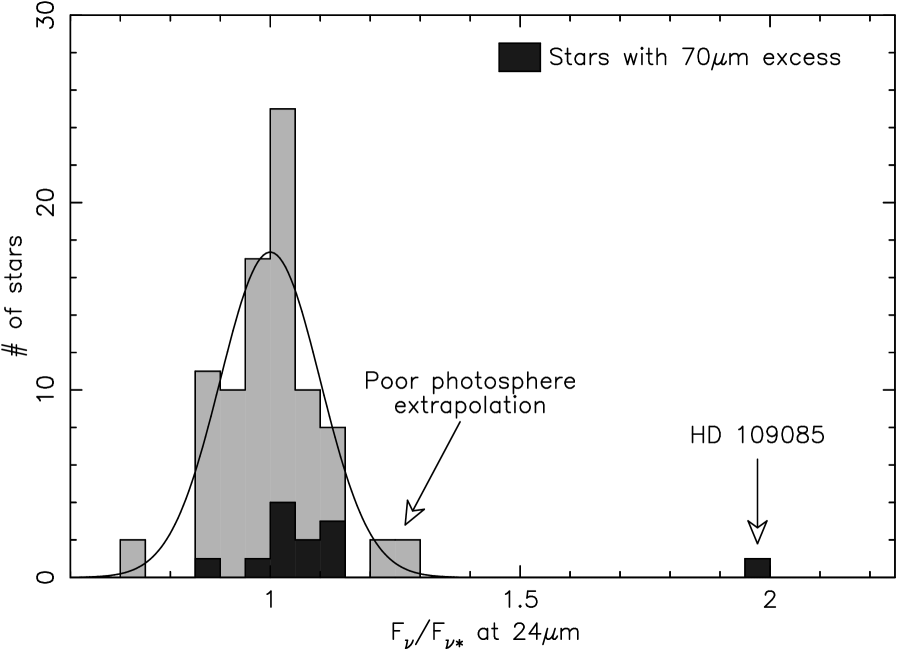
This accuracy can be directly assessed by examining how well the observed flux levels match those predicted. We use the ratio, -24µm, to assess the photospheric extrapolation using the fact previously established in Bryden et al. (2006a), Beichman et al. (2006), and earlier references cited therein, that excesses at 24 µm are rare (1%). Figure 4 shows the distribution of this ratio. After excluding one outlying star with a strong 24 µm and 70 µm excess (HD 109085), the 88 flux measurements at 24 µm have an average -24µm of 1.01. The dispersion of -24µm in Figure 4 is 0.10, which is relatively large compared to the previous result for just F5-K5 stars (0.07; Bryden et al., 2006a). We identify three causes for this larger dispersion:
3.2.1 Quality of Near-IR Photometry
The SIM/TPF sample contains a number of nearby stars that are brighter than the stars in the FGK survey. Stars brighter than about K mag have saturated 2MASS measurements resulting in large photometric uncertainties (0.25 mag). For several of these stars, particularly the early F type stars which are the brightest in the sample, Johnson -band photometry is available in the literature with much better accuracy (0.05 mag) than the saturated 2MASS values, but worse than the best 2MASS values (0.03 mag). In such cases, the saturated 2MASS values are supplanted by the better data. However, the uncertainty in the near-IR photometry for the remaining 2MASS-saturated stars causes difficulty in extrapolating to longer wavelengths and results in a greater dispersion than when only stars with high quality 2MASS data are used, (-24µm)= 0.09 vs. 0.07 for types F5-K5.
3.2.2 Intrinsic Variability
Stellar variability between the epochs of the Spitzer data and the photometry used to estimate the photospheric contribution could account for some of the dispersion in -24µm. To investigate this possibility we examined the Hipparcos photometry for the 66 stars of our sample for which these data are available (ESA 1997). Only three stars (GL 436, HD 79211 and HD 265866) showed a scatter in in excess of 0.02 mag while the vast majority had scatter less than 0.01 mag. In particular, none of the ten stars younger than 1 Gyr and thus possibly more variable than the rest of the sample, showed variability above this level. GL 436 and HD 265866 are faint V10 mag M stars so that the level of Hipparcos scatter is not significant. The large scatter for HD 79211 (0.23 mag) is due to multiplicity and is also not significant. As discussed below, one non-Hipparcos star, HD 38392, shows a low level of variability and a correspondingly larger deviation in -24µm.
3.2.3 Quality of Photospheric Models
The ability to extrapolate from visible and near-IR photometry to MIPS wavelengths appears to be an issue for spectral types later than the F5-K5 range used in the FGK survey. For all stars with accurate 2MASS data, Figure 5 plots the directly observable [24] color, a quantity independent of the stellar atmosphere models. With the exception of the M stars, all of the averages are consistent with a constant color of [24] . Most interestingly, an apparently abrupt transition occurs between the late K stars and M stars, with the average [24] color jumping up 0.4 magnitudes for the cooler stars. This trend of redder [24] for later spectral types was first noticed by Gautier et al. (2006) whose M star data are shown for comparison.
We next consider the ratio of the observed flux at 24 µm to that predicted by photospheric models (-24µm) as a function of spectral type. Solar-like stars (types F5-K4) have an overall average of -24µm with a dispersion of 5% among the stars with good 2MASS data and excluding stars with excess emission at 70 µm (identified in §3.3). For F0-F4 stars, the observed fluxes are marginally higher than those predicted, with an average -24µm . For late K stars with good 2MASS observations the observed fluxes are consistently below expectation with an average -24µm of . Since the observed K-[24] color is flat (Fig. 5), this offset is likely a fault of the photospheric modeling or of our fitting procedure. Not surprisingly, the models have the greatest difficulty with the M stars which have average -24µm = . This difference between measured and predicted fluxes for the M stars remains even if NextGen (Hauschildt et al., 1999) models are used instead of Kurucz models. However, with an accurate determination of each star’s effective temperature and with more advanced stellar models (PHOENIX; Brott & Hauschildt, 2005), Gautier et al. (2006) were able to fit the 24 µm colors of M stars.
Thus, knowing that these trends in -24µm exist and may ultimately be explained with better modeling, we can compare each star with the average Ks-[24] color within its spectral type bin (Fig. 5) to look for dust excesses. With this methodology, we find no evidence for a 24 µm excess toward any of our M stars. This negative result is strengthened when IRAC photometry is available. For the 4 M stars with IRAC data (Table 3), the inclusion of 3.5-8.0 µm fluxes into the fit modifies the average of -24µm from 1.32 with a dispersion of 0.21 to -24µm=0.92 with a dispersion 0.04, confirming that the M stars’ 24 µm fluxes are consistent with emission from the stellar photosphere alone.
3.2.4 Presence of a Weak Excess at 24
Finally, the third reason for increased dispersion in the -24µm values, in addition to poor near-IR photometry and less accurate stellar photospheres or model fitting for late type stars, is the presence of weak but real excess emission from dust toward some stars. In §3.3 we will identify some of our target stars as having strong excess emission at 70 µm. Only one of these objects, HD 109085333An excess was first detected around HD 109085 (= Crv) by IRAS (Aumann, 1988; Stencel & Backman, 1991) and subsequently with SCUBA at sub-mm wavelengths (Sheret et al., 2004; Wyatt et al., 2005). Consistency between the IRAS flux at 25 µm and the MIPS 24 µm flux measured here depends strongly on the application of color corrections which are functions of the assumed dust temperature. For dust temperatures around 200-400 K and assuming the photospheric value given in Table 2, we find good consistency between the two measurements. (the labeled value in Figure 4) also has an immediately obvious IR excess at 24 µm.
Taken in composite, however, the stars with 70 µm excesses tend to have a weak 24 µm excess. Considering only F0-K5 stars with good near-IR photometry, those with 70 µm excess have an average -24µm value 9% higher than those without. A similar general trend was previously noticed by Bryden et al. (2006a) and was confirmed in the IRS spectra of individual objects with 70 µm excess, which tend to rise above the stellar photosphere longward of 25 µm (Beichman et al., 2006). Combining the F0-K5 stars in this sample with those from Bryden et al. (2006a), we are no longer limited by small number statistics and the correlation between 70 µm and 24 µm excess becomes significant at the 3- level. The average 24 µm excess for stars with 70 µm excess is 0.0790.026 times the stellar flux.
To assess the significance of a possible 24 µm excess on a star-by-star basis, we define the parameter which corresponds to the significance of any deviation from the expected photospheric value:
| (1) |
where is the measured flux, is the expected stellar flux, and is the noise level, all at 24 µm. A similar definition follows for 70 µm (equation [2]). We take the noise to be the larger of either 4% for sources with good 2MASS or Johnson data or 8% for sources with poor near-IR photometry. These values are based on the dispersions in -24µm for the stars without 70 µm excesses. Ignoring the previously discussed late K and M stars with poor photospheric extrapolations, we find that the deviations from photospheric emission skew sharply to positive values for stars with 70 µm excess (black shading in Fig. 4). Using this analysis we identify statistically significant 24 excesses accompanying a stronger 70 excess around two stars: HD 25998 (3.6 ) and HD 40136 (3.2 ) in addition to HD 109085 discussed earlier. At slightly lower significance we find hints of a 24 excess for HD 199260 (2.7 ) and HD 219482 (1.9 ) which the accompanying 70 excess suggests could be real.
A number of other stars show strong deviations from photospheric values without an accompanying 70 µm excess: the deviant -24µm values of the M stars have already been discussed and attributed to poor photospheric extrapolation; HD 38392 has an apparent 30% excess at 24 µm which we attribute to the difficulty of obtaining an accurate measurements due to a) saturated 2MASS measurements, b) proximity to a nearby, bright companion (HD 38393) and c) the possible variability of the star itself at the 5% peak-to-peak level (Nitschelm et al., 2000). Finally, HD 23249 and HD 55892 have and . These deviations could simply be statistical fluctuations or they could be hints of an excess like that seen toward HD 69830 which is prominent only in the 8-34 region but not at 70 µm (Beichman et al., 2005a). Without additional data, e.g. IRS spectra, we cannot assess the reality of the excesses around these last two stars.
3.3 Detection of 70 µm Excess
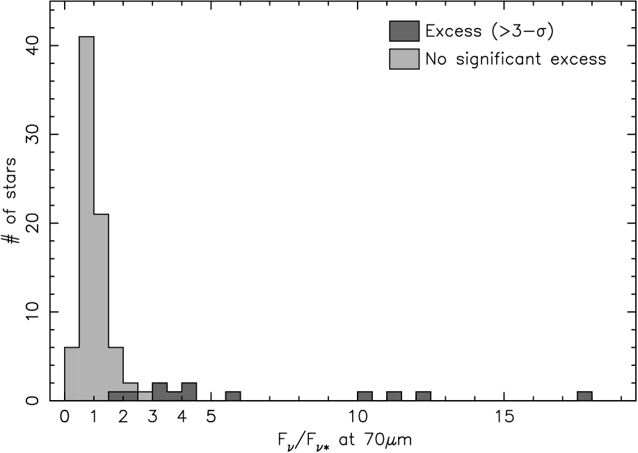
Having used 24 µm fluxes to test the accuracy of our stellar photosphere predictions, we next consider the frequency and strength of excess emission at 70 µm. The distribution of 70 µm flux densities relative to the expected photospheric values is shown in Figure 6. Unlike the tight distribution of flux ratios at 24 µm, many stars have 70 µm flux densities much higher than expected from the stellar photosphere alone. In several cases, the flux is more than an order of magnitude greater than expectation. Twelve of these stars will be identified in the following as having statistically significant IR excess. Excluding these stars with excesses and those with signal-to-noise ratio (S/N) , the average ratio of MIPS flux to predicted photosphere is -70µm, consistent with the overall calibration.
The dispersion in the 70 µm data is 40% (excluding the stars with excesses), considerably higher than that in the 24 µm data. An analysis of the noise levels in each individual field is required to assess whether the IR excesses are statistically significant. Many contributions to the overall error budget must be considered including those arising from stellar photosphere modeling, instrument calibration, sky background variation, and photon detector noise. At 70 µm, the calibration uncertainty and the background noise within each image are considerably larger than at 24 µm. On top of an assumed calibration uncertainty of 15%, we directly measure the standard deviation of the background flux when each field is convolved with our chosen aperture size. This background noise, which ranges from 2 to 20 mJy with a median of 3.7 mJy, is due primarily to extragalactic source confusion and cirrus contamination, rather than photon noise, and hence cannot be greatly reduced by additional integration time (for a more detailed analysis of the 70 µm noise levels, see Bryden et al., 2006a). Based on this measured background noise, we determine the S/N for each star, as listed in Table 2. Despite the high level of noise in some fields due to cirrus contamination and/or background galaxies, 72 out of the 87 stars in our sample with 70 µm data are detected with signal-to-noise ratio greater than 3. The median S/N for all of our target stars is 6.6, excluding the sources identified as having excess emission (which have a median S/N of over 20).
Adding both background noise and calibration error together gives us a total noise estimate for each 70 µm target. In Table 2 we list these noise levels, along with the measured and the photospheric fluxes, for each observed star. We use these noise estimates to calculate which corresponds to the significance of any deviation from the expected level of photospheric emission:
| (2) |
where is the measured flux, is the expected stellar flux, and is the noise level, all at 70 µm. Based on this criterion, we find that 12 out of 88 stars have a 3- or greater excess at 70 µm: HD 25998, HD 38858, HD 40136, HD 48682, HD 90089, HD 105211, HD 109085, HD 139664, HD 158633, HD 199260, HD 219482, and HD 219623. In a sample of 88 stars there should be fewer than 1 star with a spurious excess on purely statistical grounds. Although cirrus or extragalactic confusion could produce spurious excesses, careful examination of each of the 70 µm images suggests that
this is unlikely in the vast majority of cases. For example, the 70 µm emission is well centered on the 24 µm positions, typically within1′′. A number of weak excesses could have escaped detection under these criteria. Observations at higher sensitivity or at higher spatial resolution will be needed to identify these. The detection rate of 70 µm excess within this sample is %; combined with the sample of Bryden et al. (2006a), this gives an overall detection rate of % for cool stars.
Four of these stars have been previously identified as having excess emission: HD 40136 (= Lep; Aumann, 1988; Mannings & Barlow, 1998), HD 48682 (= 5 Aur; Aumann & Probst, 1991; Sheret et al., 2004), HD 109085 (= Crv; Aumann, 1988; Wyatt et al., 2005), and HD 139664 (= g Lup; Walker & Wolstencroft, 1988; Habing et al., 1996; Kalas et al., 2006). The eight newly discovered IR-excess stars mostly have 70 µm fluxes less than 100 mJy, too dim to have been be detected by IRAS. The notable exception is HD 105211 which has a very strong 70 µm flux (500 mJy), but lies near a bright infrared source (CL Cru); with a separation of 2.4′, this source is easily resolved in the MIPS image (Figure 7), but still contaminates the large IRAS beam. For the stars without any significant excess emission, 3- upper limits on possible excess flux typically range from 0.2 to 1.0 times the stellar flux, with a median of upper limit of 0.6 .
Although the telescope resolution at 70 µm is relatively poor (FWHM of 17′′), several of these sources appear to be slightly extended in the MIPS images (marked with superscript f in Table 2). As discussed in a separate paper (Bryden et al., 2006b), examination of the images of these marginally resolved sources do not indicate contamination by background objects, e.g. cirrus or galaxies, but rather that the objects possess to be truly extended disks. For one of the five Spitzer-resolved disks, HD 139664, a Hubble Space Telescope image shows the same orientation of the disk in the visible as in the infrared (Kalas et al., 2006). At distances of 10-20 pc, the resolved disks have apparent radii of 100’s of AU. As discussed below, maintaining a temperature of 50 K at these distances (warm enough to emit strongly at 70 µm), requires relatively small grains with low emissivities.
4 Properties of the Detected Dust
Beyond our initial goal of detecting IR excesses, we are interested in determining the properties of the dust in each system - its temperature, luminosity, mass, size distribution, composition, orbital location, etc. For the 12 stars with significant IR excess, Table 4 lists the excess 70 µm emission and measurements of or limits to the 24 µm excess. Seven of the 12 excess sources have an excess measured only at one wavelength (70 µm), restricting our ability to place limits on key quantities. The observed flux can be translated into the total dust disk luminosity relative to its parent star only when some assumption is made for the dust temperature (e.g. Beichman et al., 2005b; Bryden et al., 2006a). The minimum disk luminosity as a function of 70 µm dust flux density is obtained by setting the emission peak at 70 µm (or, equivalently, setting K):
| (3) |
Based on this equation, a minimum is calculated for each of our target stars identified as having an IR excess at only 70 µm (Table 4). For the other IR-excess stars, we also have at least a rough (2-) detection of the 24 µm excess, as discussed in the previous section. With two wavelengths of excess measurement, the dust emission can be fit with a representative dust temperature, otherwise only upper limits can be obtained (Table 4; also see Figure 11 below). Figure 8 shows a spectral energy distribution (SED) for two of these stars, HD 219482 and HD 40316, fit with temperatures of 170 and 80 K respectively. In the cases with a fit dust temperature, Table 4 lists the ratio of the integral under the stellar () and dust () blackbodies as a proper, rather than minimum, estimate of :
| (4) |
where at 70 µm.
For each of the stars with excess emission (plus those from Bryden et al. (2006a), Figure 9 shows the total dust area and radial location of the emitting material. Despite the expectation that only large grains should be seen around mature systems due to loss mechanisms such as Poynting-Robertson drag and radiation pressure, small grains must be considered as a serious possibility given their presence in a mature star like HD 69830 (Beichman et al., 2006) and because of the large extent of at least some the dust disks. Thus, the orbital location of the emitting material can only be calculated if some assumption is made for the dust’s emissivity; small grains are less efficient at emitting infrared radiation, resulting in a higher temperature for a given orbital radius. For a given dust temperature, the orbital radius decreases with emissivity as . As such, for each calculated dust temperature or upper limit in Table 4, two locations are plotted - the location if the emitting material is large blackbodies (lower axis) and the location if it is small grains with emissivity = 0.01 (upper axis).
The dust area and mass have a similar ambiguity based on the unknown dust size/emission properties. The dust area in Figure 9 (left axis) is calculated under the assumption of blackbody grains (unity emissivity); a lower emissivity would increase the dust area in direct proportion to . Lastly, the dust mass (right axis) is based on an assumed typical grain size of 10 µm. An unconstrained amount of mass is contained in the larger parent bodies whose collisions produce the emitting dust.
For stars with no detected emission, 3- upper bounds on the 70 µm fluxes lead to upper limits on as low as a few times , assuming a dust temperature of 50 K (Table 2). Although we cannot rule out cold dust at 100 AU, we are placing constraints on dust at Kuiper Belt distances to 10-100 times the level of dust in our solar system. The constraint on asteroid belt-type dust is less stringent, 100-1000 times our zodiacal emission.
4.1 Comparison with Sub-mm Observations
The dust properties can be further constrained with sub-mm flux measurements. When available, longer wavelength data can help place lower limits on dust temperature, upper limits on the dust luminosity, and, with some assumption on the grain emissivity, outer limits on the disk extent. For most of our stars with IR excess, large amounts of cold dust emitting at longer wavelengths cannot be ruled out, but three of the 70 µm excess stars have been observed at 450 and 850 µm with JCMT/SCUBA, with two detections (HD 48682 and HD 109085) and one upper limit (HD 139664; Sheret et al., 2004). Combining their sub-mm data with the infrared fluxes from IRAS, Sheret et al. (2004) modeled the SEDs for these stars, obtaining dust temperatures of 99 and 85 K for HD 48682 and HD 109085, respectively.
4.2 Comparison with Visible Observations
A nearly edge-on disk around HD 139664 has recently been detected at visible wavelengths using the Hubble Space Telescope (HST) (Kalas et al., 2006). The HST image of the disk shows a well defined inner edge around 83 AU and an outer edge that extends out to about 109 AU. If the dust associated with the 70 µm emission is located in this ring, then a very large surface area of 10 grains would be required for the IR emission, since dust at this distance would have an equilibrium temperature of 30-35 K using a standard radial power law for grain temperature (Beichman et al., 2006). Smaller, 0.25 grains, on the other hand, give temperatures of 69 and 77 K at the ring boundaries (cf. our 3-sigma upper limit of 78 K; Table 4). Using a simple relationship for dust mass, , and standard silicate absorption efficiencies, (Draine & Lee, 1984; Beichman et al., 2006), yields a mass of in large grains or in small grains, where we have taken a grain density of =3.3 gm cm-3 and a distance, pc, for this star.
The radiative blowout size for grains around an F5 star is approximately 1 µm (§V.B.1 in Backman & Paresce (1993); Burns et al. (1979)). In contrast to the spherical distribution of small grains seen toward Vega (Su et al., 2005) which is probably due to a recent catastrophic event, small grains should be quickly ejected from the presumably stable ring system of HD 139664. IRS spectroscopy and/or millimeter spectroscopy would help distinguish between the large and small grain models.
5 Correlation of Excess with System Parameters
To understand the origin and evolution of infrared excess, we now consider the properties of the sample stars and how they correlate with excess detection. Specifically, we examine the correlation with three variables: metallicity, age, and spectral type. These parameters are listed for each star in Table New Debris Disks Around Nearby Main Sequence Stars: Impact on The Direct Detection of Planets. Where appropriate we merge the present sample with that of Bryden et al. (2006a) to improve the significance of any statistical conclusions.
5.1 Metallicity
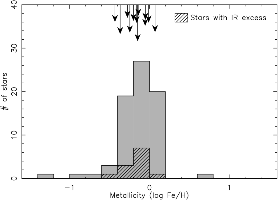
Table New Debris Disks Around Nearby Main Sequence Stars: Impact on The Direct Detection of Planets lists the metallicity information obtained from the literature for each of our target stars (number of independent [Fe/H] estimates, their average, and their r.m.s. scatter). Figure 3 shows a histogram of these metallicity values, the majority of which range between - 0.4 to +0.1 dex with a mean value of somewhat below solar. The stars with IR excess are identified with vertical arrows with the length of each arrow proportional to the strength of 70 µm excess. We find no correlation between metallicity and IR excess. The average [Fe/H] is -0.150.03 for all the observed stars and -0.170.04 for the stars with excess - an insignificant difference.
These data are combined with Bryden et al. (2006a) sample to show the fractional incidence of disks as a function of [Fe/H] (Figure 12). A test shows that the distribution of disks in our three metallicity bins with significant number of stars (-0.75 [Fe/H] 0.0) is indistinguishable from flat. The lack of correlation between IR excess and metallicity is in sharp contrast with the well known correlation between extrasolar gas giant planets and host star metallicity (Gonzalez, 1997; Santos et al., 2001). In particular, Fischer & Valenti (2005) find that the probability of harboring a radial-velocity detected planet increases as the square of the metallicity (Figure 12). Although one might suspect giant planets and debris disks to be related, a similarly strong correlation between dust and metallicity can be confidently ruled out. A comparison between the disk and planet distributions in same 3 [Fe/H] bins suggest that there is only a 0.3% probability of these being drawn from the same distribution.
The lack of correlation is further confirmed via Monte Carlo simulations. Again using our dataset combined with that of Bryden et al. (2006a) (giving a total of 19 excess stars out of 151 observed), the correlation coefficient, , is calculated for 10,000 random samples of stars. The histogram of the resultant values is shown in Figure 13 under two different assumptions. In one case, the stars with excess are chosen randomly (left histogram centered on =0); in the other, the stars are chosen with weighting proportional to their metallicity squared (right histogram with average =0.33). The correlation coefficient observed within our data (vertical arrow) is inconsistent with the strong metallicity dependence observed within planet-bearing stars.
This lack of correlation may reflect the different formation histories of giant planets and debris disks. The accretion of gas onto a giant planet requires a large solid core to form first, favoring a higher metallicity disk, whereas dust emission indicates the presence of smaller planetesimals that might be able to form in all disk environments. Another explanation may be that debris disks in high metallicity systems initially contain more material, but that over time all disks grind down toward similar masses (e.g. Dominik & Decin, 2003). In this case, the detection of strong IR emission is a reflection of a recent stochastic collision, rather than the disk’s initial conditions (see Bryden et al. (2006a) for further discussion).
5.2 Age
Collisions in a debris disk continually grind down the larger planetesimals, while the smallest dust can be removed by Poynting-Robertson drag and radiation pressure. One would assume that the overall disk mass must decline with time and, as expected, a correlation between stellar age and IR excess is observed, with debris disks more commonly identified around younger stars. While studies concentrating on stars younger than 1 Gyr find a strong trend (Spangler et al., 2001; Rieke et al., 2005), among nearby solar-type field stars the correlation is relatively weak (Bryden et al., 2006a). In both cases, the evolution of the dust does not appear to be a steady decline. Observations of A stars find an overall decline in the average amount of 24 µm excess emission on a 150 Myr time scale, but the large variations on top of this trend suggest that sporadic collisional events are able to dramatically increase the amount of dust even at late stages in the disk’s evolution (Rieke et al., 2005). As a result of these collisions, even old stars can have strong IR emission (Habing et al., 2001; Decin et al., 2000; Bryden et al., 2006a).
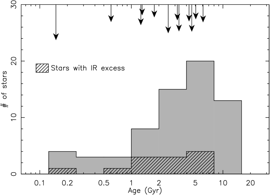
Figure 2 shows the resultant histogram of stellar ages. The ages for our main sequence stars are difficult to determine, with uncertainties in many cases of at least a factor of two. Where possible, we use ages based on Ca II H&K line emission from the large compilation of Wright et al. (2004). Otherwise an average of values found in the literature is used. If the star was inferred to be young due to kinematic properties (Montes et al., 2001), we adopted that age. Table New Debris Disks Around Nearby Main Sequence Stars: Impact on The Direct Detection of Planets lists the age data for each star. Although our target selection criteria do not explicitly discriminate based on stellar age, young stars (ages less than 1 Gyr) are not well represented in our sample due to their infrequent occurrence within 25 pc of the Sun.
As in our earlier survey of nearby main-sequence stars (Bryden et al., 2006a), the stars with excess in this survey (marked with arrows in Figure 2) have a weak but noticeable correlation with stellar age. No stars older than 7 Gyr have a significant amount of excess emission. The average age of stars with IR excess is 4.00.6 Gyr, compared to 5.60.4 Gyr for the sample as a whole. As discussed in the next section, these trends are present in the combination of this sample with the Bryden et al. (2006a) data.
5.3 Spectral Type
Observations of the general characteristics of debris disk as a function of spectral type are potentially a powerful tool for understanding the physical mechanisms responsible for the evolution of debris disks. The disk properties should be directly related to the stellar mass and luminosity in several ways. The mass of the protostellar disk from which the debris formed, for example, probably depends on the parent star’s mass, as does its dynamical time scale. The stellar luminosity, though, is undoubtedly more important for debris disk characteristics, exerting a strong influence on the typical particle size () as well as its temperature (). There are also observational biases linked to the brightness of the star, with cool dust seemingly easier to distinguish around hotter stars.
The minimum based on the 70 µm flux, for example, is strongly dependent of stellar temperature (in eq. [3], detectable is proportional to ). Hotter stars emit a lower fraction of their luminosity at infrared wavelengths, allowing for better contrast at those wavelengths. But while equation (3) is an observationally well-defined quantity, it contains no knowledge of the underlying disk physics. Naively, it appears to dictate a strong relationship between detectability and spectral type, i.e. it is easier to detect dust around hotter stars, but this may be misleading. For lack of any other information, the equation assumes that the dust emission peaks at 70 µm, thereby measuring the minimum . This assumed SED shape corresponds to a fixed dust temperature of 50 K for all disks. One can instead consider disk models with a more physically motivated dependence on spectral type. Instead of assuming a constant dust temperature, Habing et al. (2001), for example, assume the same dust location for all disks; in their models, the dust resides at 50 AU independent of spectral type. In this case, dust temperature decreases with . In contrast with a simple reading of equation (3), the Habing et al. models have more or less directly proportional to for stars of type G and earlier. As in equation (3), lower stellar temperature makes it more difficult to detect dust emission relative to the stellar photosphere, but in Habing et al.’s models this difficulty is offset by a lower dust temperature for cooler stars, increasing the dust’s 70 µm emission.
In Figure 1, the spectral types with IR excess stars are flagged with vertical arrows. A clear trend is readily apparent, with excess more frequently detected around earlier type stars. The detection rate drops from nearly 30% for the earliest type stars down to 0% for M stars. In fact, no stars with spectral type later than K0 are found to have excess emission (a sample of 23 stars without excess). This is consistent with previous survey results that considered only part of the spectral range covered here. Our survey of F5-K5 stars (Bryden et al., 2006a) found a detection rate of 13% within this limited spectral range, while a sample of 30 images of nearby M stars yielded none with IR excess at 70 µm (Gautier et al., 2006).
A possible interpretation of the trend with spectral type is that it simply reflects the known correlation with stellar age. Earlier spectral type stars tend to be younger. Figure 10 combines information on spectral type and age into a single plot for stars in this survey and those of Bryden et al. (2006a). The trends previously identified are apparent - an upper limit to the ages of stars with excesses (filled symbols) of about 6 Gyr and a tendency for earlier type stars to have excess more frequently than later types. While the earliest type stars (F0-F3) are clearly younger on average, there is no clear evidence within the bulk of the sample that higher mass stars have more frequent excess because of they have younger ages. The formal correlation of excess with spectral type is even stronger than the correlation with age (correlation coefficients are -0.200.08. and -0.150.08 for spectral type and age respectively), further suggesting that spectral type is an independent indicator for IR excess. Unfortunately many of the latest type stars lack reliable age indicators, making it difficult to make any stronger conclusions.
5.3.1 Comparison with Early Type Stars
The detection rate of 70 µm excess around A stars is 334% (Su et al., 2006), more than twice that for the stars considered in this paper (133%). However, the A star and FGK star samples differ in both mass and age. We first consider the possibility that the different detection rates simply reflect an age evolution, rather than a spectral type dependence. For example, the youngest FGK stars have a detection rate somewhat higher than that within the sample as a whole: considering only systems with ages of 0.1-1 Gyr (and including the stars from Bryden et al. (2006a)), 5 out of 19 young FGK stars have excess 70 µm emission (= 2612%). Similarly, the 70 µm excess frequency among the A stars drops with stellar age down to just 216% for A stars 0.3 - 1 Gyr old (Su et al., 2006). It is important to note, however, that many of the Su et al. (2006) observations are less sensitive than those presented here, relative to the stellar photosphere. Thus, their A star detection rate should be regarded as a lower limit. Although the FGK and A star samples have stellar age as the most important correlating factor for IR excess, we cannot rule out a weaker but still important dependence of IR excess on some factor related to stellar mass such as luminosity or disk mass.
5.3.2 Comparison with Late Type Stars
Combining the observations presented here with those of Bryden et al. (2006a) and Gautier et al. (2006), we have a total sample of 61 K1-M6 stars with no evidence of excess emission at 70 µm. Even considering only those stars whose photospheres are detected at 70 µm with S/N3 (42 of the 61 stars), this lack of excess detections is 3- inconsistent with the 15% detection rate around F and G type stars. As implied by Eqn (3), the contrast of dust relative to photosphere is, however, poorer for cooler stars which emit more of their energy in the infrared than hotter stars. The average upper limit to for the 16 stars K1 or later with detected photospheres but no excesses in the SIM/TPF sample ( and ) is compared with the average upper limit for 51 hotter stars with detected photospheres but no excesses, . Thus, one explanation for the lack of excesses around later-type stars is simply that the effective observational limits are a factor of two higher for the cooler stars. While observational selection effects make detection of IR excess around late type stars more difficult, the strength of this trend suggests that other explanations are needed.
Another ambiguity in interpreting the correlation of excess with spectral type results from our limited knowledge of the location of the dust. If dust around later type stars is very distant from its central star, it will be too cool for detection at 70 µm. Figure 11 shows how the dust temperature varies as a function of spectral type for stars with excess from both this sample and from Bryden et al. (2006a). We can only derive a dust temperature in the limited number of cases where we have a measured excess at both 24 and 70 µm (solid points). Otherwise, only upper limits can be obtained (Table 4). For unresolved disk observations, the dust location cannot be determined without some knowledge of the underlying dust emission properties. Smaller dust with low emissivity can be just as hot as larger grains closer to the central star. Lines of constant orbital radius are shown in Figure 11 under the assumption of either large blackbody grains () or of small grains with emissivity = 0.01. Although the observed temperatures range from 80 to 170 K, they are all more or less consistent with emission from similar orbital locations: 10 AU for or 100 AU for . By implication, one would expect that dust around later K stars might have typical temperatures of 50 K, ideal for detection at 70 µm, though none were detected.
Additional information on the location of the dust comes from IRS observations of F, G, and K stars with excesses (Beichman et al., 2006) which reveal that in almost all cases the inner boundary of the emitting region occurs at or interior to 10 AU. A theoretical basis for this preferred location of a radial distance of a few AU comes from the suggestion that the water-ice sublimation distance, or the “snowline” where the temperature falls below 170 K, should mark the onset of the region of giant planet formation and its remnants in the Kuiper Belt (Hayashi, 1981; Sasselov & Lecar, 2000; Garaud & Lin, 2006). Since the location of the snowline varies with stellar luminosity (), there is no reason to expect a more distant, hidden reservoir of material unsampled by our observations around cooler stars. It is, of course, important to verify this expectation with observations at longer wavelengths such as MIPS 160 m and in the sub-millimeter. Within the Gautier et al. (2006) sample, for example, none of the 20 M stars examined at 160 µm show any excess emission, providing limits on of -10-3 for material at 50 AU.
If the lack of debris disks around cool stars is real, then the dearth of material might reflect different formation mechanisms and evolutional history for the belts of planetesimals around low mass stars. Dust-producing collisions within these belts, for example, may require planetesimal stirring by larger, gas-giant planets, whose frequency is thought to be lower for late-type stars (Laughlin et al., 2004), Alternately, the lack of IR excess might instead indicate a change in the physics of the smallest orbiting bodies as later type stars are considered, such as the increased relative importance of stellar winds in clearing dust from the system (Plavchan et al., 2005).
6 Applicability to TPF
The detection of other terrestrial planets is a long term goal for the astronomical community (McKee & Taylor, 2001). NASA has spent considerable funds over the past decade on technology development and mission studies for a Terrestrial Planet Finder (TPF). One of the key astro-engineering issues revealed by those studies is the level of dust emission associated with target stars since exo-zodiacal emission is potentially an important source of photon shot noise (Beichman et al., 1999). Thus, in addition to scientific interest, the incidence and distribution of material in the habitable zones, i.e. where planets might have surface temperatures consistent with the presence of liquid water (Kasting et al., 1993), of nearby stars is of considerable technical importance.
6.1 Effect of Exo-Zodiacal Dust on Planet Finding
As discussed in Appendix A, dust emission at the level of 10-20 times that of our own zodiacal cloud can impede planet searches (Figure 15) due to increased photon shot noise for either a coronagraph or an interferometer. Since this level is roughly 50-100 times less than that presently detectable with Spitzer, we can rule out only those stars with the most extreme zodiacal disks. Thus, HD 109085 and HD 69830 (Beichman et al., 2005a) are unsuitable targets with strong excess shortward of 24 µm. However, the remaining stars in this sample and other samples pass the initial screening by having 24 µm excesses, if any, less than , corresponding to upper limits on 500 (Bryden et al., 2006a). Beyond these photometric constraints, IRS spectroscopy can push upper limits to factors of 2-3 lower than MIPS alone and can also identify stars with small grain emission at 10 m (Beichman et al., 2006).
In a few cases listed in Table 6 we can use the blackbodies fitted to the emission from the 5 stars with data at both
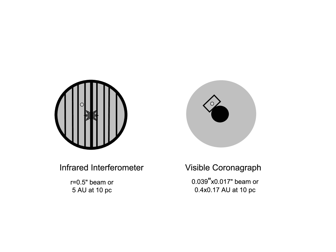
24 and 70 (Table 4) to extrapolate the emission from this “Kuiper Belt” dust to the prime TPF-I wavelength of 10 . The extrapolated emission is also given in units of for material emitting at 10 (cf. eq. [3] and eq. [2] of Beichman et al. (2006)) relative to the solar system value of (Backman & Paresce, 1993). Emission from any of this material located within the primary beam of the TPF-I telescopes (5 AU for a star at 10 pc observed with 3 m apertures) would be a noise source as described in the Appendix. However, this population of “cool” or “lukewarm” grains would not be located within a TPF-C pixel centered on the 1 AU habitable zone and would not be a noise source at visible wavelengths.
Unfortunately, however, the present observations cannot rule out an additional population of hotter grains located closer to the star which would either emit at 10 or scatter in the visible. IRS observations in the 8-14 m region reach levels of just 1,000 times the zodiacal level (Beichman et al., 2006). It will take observations with nulling Interferometers such as the Keck and Large Binocular Telescope Interferometers which can spatially suppress the stellar component to measure directly the exo-zodiacal emission in the habitable zone at levels that could cause S/N or confusion problems for TPF.
There is some cause for optimism, however. The “luminosity function” of disks inferred from a variety of Spitzer samples (Bryden et al., 2006a), the rarity of extreme “hot” zodiacal disks in the sample reported here and in other Spitzer papers (Bryden et al., 2006a; Beichman et al., 2006), and the apparent decline in the number of stars with excesses as a function of age (Fig. 2) are all encouraging signs that the relatively clean example of our solar system may be the norm rather than the exception. The ring-like structures seen in a number of resolved Spitzer disks, e.g. Fomalhaut (Stapelfeldt et al., 2004) and Eri (Backman et al., in preparation) as well as in HST images (Kalas et al., 2005, 2006) suggest that although the regions interior to the rings may not be completely empty due to a variety of mechanisms capable of transporting material inward from the outer disk (comets, PR drag, interactions with planets, etc.; Holmes et al., 2002), these interior regions may have a quite low total optical depth, perhaps as low as the 20% contribution inferred for material from Kuiper Belt material to the total amount seen at 1 AU in our solar system (Landgraf et al., 2002; Dermott & Kehoe, 2004; Moro-Martín & Malhotra, 2005).
7 Summary
We have searched for circumstellar dust around a sample of 88 F-M stars, by means of photometric measurements at 24 µm and 70 µm. We detected all the stars at 24 µm with high S/N and more than 80% of the stars at 70 µm with S/N . Uncertainties in the Spitzer calibration and in the extrapolation of stellar photospheres to far-IR wavelengths limit our ability to detect IR excesses with 3- confidence to 20% and 50% of the photospheric levels at 24 and 70 µm, respectively.
At these levels we have detected 12 of 88 objects with significant 70 µm excesses. Combined with an earlier study (Bryden et al., 2006a), we find an overall detection rate of % for mature cool stars. Beyond the single previously known 24 µm excess within our sample, we detect two objects with 70 µm excesses and definite but weak 24 µm emission. Another two stars with 70 µm excesses have hints of 24 µm excesses. These results build on the finding of Beichman et al. (2006) that in many cases, objects with 70 µm emission also had IRS spectra rising longward of 25 to meet the 70 µm excess. These objects are all consistent with a disk architecture similar to our Kuiper Belt that is concentrated outside 5-10 AU. In this context we note that a number of the 70 µm sources are slightly, but significantly extended at 70 µm. The detailed discussion of these objects is deferred to a subsequent paper (Bryden et al., 2006b). The IR emission in these systems is different from the exceptional object HD 69830, which shows a disk architecture much more consistent with a massive asteroid belt (Beichman et al., 2005a).
Cross-correlating the detections of IR excess with stellar parameters we find no significant correlations in the incidence of excesses metallicity, but do find weak correlations with both stellar age and spectral type. The lack of correlation with metallicity contrasts with the known correlation between planet detections and stellar metallicity, and the expectation that higher metal content might result in a greater number of dust-producing planetesimals.
One significant finding is that the incidence of debris disks among mature stars is markedly lower for spectral types later than K0 than for earlier spectral types. Combining data from this survey, the Bryden et al. (2006a) F5-K5 survey, and the Gautier et al. (2006) M star survey suggests an incidence of disks of 3% for F0-K0 stars and 4% for stars with types K2-M3. This lack of disks around later spectral types may be due to selection effects, lower initial disk mass, or different rates of dust creation or destruction.
The disks that we are detecting have typical 70 µm luminosities around 100 times that of the Kuiper Belt. If they also have inner asteroid belts 100 times brighter than our own, however, we would still not be able to detect this warm inner dust. The observed 70 µm excess systems could all be scaled-up replicas of the solar system’s dust disk architecture, differing only in overall magnitude. These systems could have planets, asteroids and Kuiper Belt Objects as in our own system, but simply with a temporarily greater amount of dust due to a recent collisional event. Further observations of the warmer inner dust are necessary to address this possibility. Spitzer/IRS is particularly promising in this regard (Beichman et al., 2006) and is being pursued as part of a follow-up effort for some of the stars in this program.
Appendix A Noise Due to Exo-Zodiacal Emission
In this section we make order of magnitude estimates of the impact of photon noise from exo-zodiacal emission on both visible light and mid-IR instruments (TPF-Coronagraph and TPF-Interferometer, respectively) designed to find neighboring planets. A detailed noise analysis of planet finding telescopes is beyond the scope of this paper and the reader is referred to other articles for more details (Beichman & Velusamy, 1999; Brown, 2005).
A.1 TPF-I, The Infrared Interferometer
The use of a nulling interferometer to reject starlight and thereby reveal an orbiting planet dates to an article by Bracewell (1978) and has been further investigated through studies of more sophisticated configurations (Angel & Woolf, 1997; Lay et al., 2005). For a cryogenic system operating in an orbit near 1 AU, the three dominant noise sources are (Beichman & Velusamy, 1999, Table 5): the stellar light that leaks past the interferometric null because of the finite diameter of the star, S∗,Leak; emission from the local zodiacal dust, SLZ; and emission from the exo-zodiacal dust in the target star system that leaks past the interferometer, SEZ,Leak (see Figure 14). At short wavelengths (8 ), the stellar leak may dominate all other noise sources; longward of 20 emission from a 35 K telescope will become important; and at all wavelengths various systematic instrumental effects will be important. But over a broad range of wavelengths, the balance between S∗,Leak, SLZ, SEZ,Leak controls the fundamental noise floor. Detector read noise and dark current can be ignored for broad band detection.
In the background limit considered here, the total noise is given by the square root of the sum of all the individual photon fluxes reaching the detector. Rather than evaluate the absolute signal-to-noise ratio, S/N, we consider here the ratio of the S/N in the presence of exo-zodiacal emission, SNR(EZ), to the S/N in the absence of such emission, SNR(0):
| (A1) |
In the above, depends on the nulling configuration, the wavelength of operation and the angular size of the star. Null depths of to have been demonstrated in the laboratory (Martin et al., 2003) and for the purposes of this illustration, it suffices to take . The emission from the local zodiacal cloud, , is very complex in detail (Kelsall et al., 1998), but can be parameterized for our purposes as follows, where is the Planck function, is the vertical optical depth looking out from the mid-ecliptic plane at 1 AU, and is the diffraction limited solid angle of an individual telescope in the interferometer. A typical value of the zodiacal cloud brightness toward the ecliptic pole from our mid-plane location is 12 MJy sr-1 at 12 (Kelsall et al., 1998).
In the absence of more detailed information, the vertical optical depth of the exo-zodiacal dust in any system can be parameterized as a factor, , times the Solar System’s zodiacal dust. The emission from exo-zodiacal dust is then , where the factor of two accounts for the fact that in the exo-zodiacal case we are looking through the entire cloud and not from the vantage of the mid-plane as we do the local cloud. By analogy with the local zodiacal cloud (Backman, 1998) the vertical optical depth is assumed to fall off radially as . We also take as the equilibrium temperature for grains heated by stellar radiation and emitting in the infrared. Typical 1 AU values of (, ) for large and small silicate grains are (255 K, -0.5) and (362 K, -0.4), respectively (Draine & Lee, 1984; Backman & Paresce, 1993; Beichman et al., 2006). The large and small grain brightness distributions are normalized to yield the same value at 1 AU.
The effect of exo-zodiacal emission is modulated by the fringe pattern of the interferometer which attenuates the bright central portion of the exo-zodiacal disk. To account for this effect we incorporate the fringe pattern of a particular nulling scheme where and are the radial and azimuthal variables, respectively. In the simplified case of a face-on disk, the signal reaching the detector, SEZ,Leak is then given by the integral of SEZ over the fringe pattern and the telescope solid angle:
| (A2) |
for a star at a distance . We adopt the fringe pattern for the Dual Chopped Bracewell interfermoter (DCB; Lay, 2004; Lay et al., 2005) presently under study. Canceling out common factors, the stellar leak term in equation (A1) then becomes
| (A3) |
To evaluate equation (A3), we adopt a diffraction limited beam size of for a 3 m telescope at 12 . For a solar-type star at 10 pc, the ratio of the exo-zodiacal contribution to that from the Solar System’s own dust (eq. A3) is 0.06 or 0.24 , for large and small grains respectively. Warmer, smaller grains fill more of the beam of the individual telescopes than the cooler, larger (blackbody) grains and thus contribute more noise. With this information in hand, Figure 15 shows the variation of S/N as a function of exo-zodiacal brightness, , for two grain sizes. When the exo-zodiacal surface density is 10 times that of our solar system, corresponding to a 20-fold brightness increase, the S/N is reduced by a factor of 2, necessitating an increase in integration time by a factor of 4 to recover the original S/N. It is interesting to note the importance of grain size on this effect; the emission from the large grains is more centrally peaked and thus more effectively attenuated by the nulling interferometer than for the smaller grains which remain warm at quite large distances from the star. Since at least a few hours of integration time is needed to detect an Earth in the presence of a cloud, and days to carry out a spectroscopic program (Beichman, 1998; Lay et al., 2005), it is clear that studying systems with will be difficult.
A.2 TPF-C, the Visible Light Coronagraph
A similar analysis can be applied to an assessment of the effects of exo-zodiacal emission at visible wavelengths. There are some important differences however. First, the coronagraph takes in only the exo-zodiacal light from the immediate vicinity of the planet, not from the entire exo-zodiacal cloud (Fig. 14, right side). Second, the signal from an Earth (), the residual starlight after a 10-10 rejection ratio, and the local and exo-zodiacal signals are all more evenly balanced. Detector noise becomes a serious issue at medium spectral resolution (75), but can be ignored in the broadband case. The analog of equation (A1) for the coronagraph becomes:
| (A4) |
Since the local and exo-zodiacal emission enter the system through exactly the same solid angle, , the term simplifies to 2. For a planet 25 mag fainter than a V=4.5 mag solar twin at 10 pc, and assuming a local zodiacal brightness of 0.1 MJy sr-1 at 0.55 (Table 5; Bernstein et al., 2002), we can evaluate the variation in S/N as a function of . Figure 15 shows the decrease in S/N as the exo-zodiacal emission increases in the case of a face-on disk; an edge-on disk will increase the surface brightness and resultant noise. As with the interferometer, the effect of zodiacal emission in the target system is to lower the S/N by a factor of 23 at
The relative effect of the exo-zodiacal emission is somewhat more pronounced for the TPF-C than for the TPF-I because the interferometer is dominated by the strong local zodiacal background until very bright exo-zodiacal levels are observed. The intrinsic background level within the visible-light coronagraph is low (by assumption of an excellent 10-10 rejection ratio) so that the exo-zodiacal emission more quickly plays a significant role in setting the system noise.
A more detailed examination of the effects of the exo-zodiacal emission on the detectability of planets using TPF-C and TPF-I would yield absolute, not relative, sensitivity levels including the effects of disk inclination and confusion by structures, e.g. wakes and gaps, within the zodiacal cloud. These questions lie beyond the scope of this paper.
References
- Angel & Woolf (1997) Angel, J. R. P. & Woolf, N. J. 1997, ApJ, 475, 373
- Aumann (1988) Aumann, H. H. 1988, AJ, 96, 1415
- Aumann & Probst (1991) Aumann, H. H. & Probst, R. G. 1991, ApJ, 368, 264
- Backman (1998) Backman, D. E. 1998, in Exozodiacal Dust Workshop:, 107
- Backman & Paresce (1993) Backman, D. E. & Paresce, F. 1993, in Protostars and Planets III, 1253–1304
- Barry (1988) Barry, D. C. 1988, ApJ, 334, 436
- Beichman (1998) Beichman, C. A. 1998, in Proc. SPIE Vol. 3350, p. 719-723, Astronomical Interferometry, Robert D. Reasenberg; Ed., 719–723
- Beichman et al. (2005a) Beichman, C. A., Bryden, G., Gautier, T. N., et al. 2005a, ApJ, 626, 1061
- Beichman et al. (2005b) Beichman, C. A., Bryden, G., Rieke, G. H., et al. 2005b, ApJ, 622, 1160
- Beichman et al. (2005c) Beichman, C. A., Bryden, G., Stapelfeldt, K. R., et al. 2005c, in Protostars and Planets V, Proceedings of the Conference held October 24-28, 2005, in Hilton Waikoloa Village, Hawai’i. LPI Contribution No. 1286, 8574
- Beichman et al. (2006) Beichman, C. A., Tanner, A., Bryden, G., et al. 2006, ApJ, 639, 1166
- Beichman & Velusamy (1999) Beichman, C. A. & Velusamy, T. 1999, in ASP Conf. Ser. 194: Working on the Fringe: Optical and IR Interferometry from Ground and Space, 408
- Beichman et al. (1999) Beichman, C. A., Woolf, N. J., & Lindensmith, C. A. 1999, The Terrestrial Planet Finder (TPF) : a NASA Origins Program to Search for Habitable Planets (National Aeronautics and Space Administration : Jet Propulsion Laboratory publication ; 99-3)
- Bernstein et al. (2002) Bernstein, R. A., Freedman, W. L., & Madore, B. F. 2002, ApJ, 571, 85
- Bowell (1996) Bowell, E. 1996, VizieR Online Data Catalog, 1, 2001
- Bracewell (1978) Bracewell, R. N. 1978, Nature, 274, 780
- Brott & Hauschildt (2005) Brott, I. & Hauschildt, P. H. 2005, in ESA SP-576: The Three-Dimensional Universe with Gaia, ed. C. Turon, K. S. O’Flaherty, & M. A. C. Perryman, 565
- Brown (2005) Brown, R. A. 2005, ApJ, 624, 1010
- Bryden et al. (2006a) Bryden, G., Beichman, C. A., Trilling, D. E., et al. 2006a, ApJ, 636, 1098
- Bryden et al. (2006b) Bryden, G., Tanner, A., Beichman, C. A., et al. 2006b, ApJ, in preparation
- Burns et al. (1979) Burns, J. A., Lamy, P. L., & Soter, S. 1979, Icarus, 40, 1
- Butler et al. (2004) Butler, R. P., Vogt, S. S., Marcy, G. W., et al. 2004, ApJ, 617, 580
- Carpenter et al. (2006) Carpenter et al., J. 2006, ApJ, in preparation
- Cayrel de Strobel et al. (1996) Cayrel de Strobel, G., Soubiran, C., Friel, E. D., Ralite, N., & Francois, P. 1996, VizieR Online Data Catalog, 3200, 0
- Cayrel de Strobel et al. (2001) Cayrel de Strobel, G., Soubiran, C., & Ralite, N. 2001, VizieR Online Data Catalog, 3221, 0
- Chen et al. (2001) Chen, Y. Q., Nissen, P. E., Benoni, T., & Zhao, G. 2001, VizieR Online Data Catalog, 337, 10943
- Decin et al. (2000) Decin, G., Dominik, C., Malfait, K., Mayor, M., & Waelkens, C. 2000, A&A, 357, 533
- Dermott & Kehoe (2004) Dermott, S. F. & Kehoe, T. J. J. 2004, in ASP Conf. Ser. 324: Debris Disks and the Formation of Planets, ed. L. Caroff, L. J. Moon, D. Backman, & E. Praton, 143
- Dominik & Decin (2003) Dominik, C. & Decin, G. 2003, ApJ, 598, 626
- Draine & Lee (1984) Draine, B. T. & Lee, H. M. 1984, ApJ, 285, 89
- Eggen (1998) Eggen, O. J. 1998, AJ, 115, 2397
- Fajardo-Acosta et al. (2000) Fajardo-Acosta, S. B., Beichman, C. A., & Cutri, R. M. 2000, ApJ, 538, L155
- Feltzing et al. (2001) Feltzing, S., Holmberg, J., & Hurley, J. R. 2001, VizieR Online Data Catalog, 337, 70911
- Fischer & Valenti (2005) Fischer, D. A. & Valenti, J. 2005, ApJ, 622, 1102
- Garaud & Lin (2006) Giraud, P. and Lin, D. N. C. 2006, ApJ, submitted
- Gautier et al. (2006) Gautier et al., T. N. 2006, ApJ, in preparation
- Giorgini (2005) Giorgini, J. D. 2005, in http://ssd.jpl.nasa.gov/ispy.html
- Gonzalez (1997) Gonzalez, G. 1997, MNRAS, 285, 403
- Gordon et al. (2005) Gordon, K. D., Rieke, G. H., Engelbracht, C. W., et al. 2005, PASP, 117, 503
- Gordon et al. (2004) Gordon, K. D., Engelbracht, C. W., Muzerolle, J., et al. 2004, in Microwave and Terahertz Photonics. Edited by Stohr, Andreas; Jager, Dieter; Iezekiel, Stavros. Proceedings of the SPIE, Volume 5487,(2004)., ed. J. C. Mather, 177–185
- Habing et al. (1996) Habing, H. J., Bouchet, P., Dominik, C., et al. 1996, A&A, 315, L233
- Habing et al. (2001) Habing, H. J., Dominik, C., Jourdain de Muizon, M., et al. 2001, A&A, 365, 545
- Hauschildt et al. (1999) Hauschildt, P. H., Allard, F., & Baron, E. 1999, ApJ, 512, 377
- Hayashi (1981) Hayashi, C. 1981, Progress of Theoretical Physics Supplement, 70, 35
- Holmes et al. (2002) Holmes, E. K., Dermott, S. F., & Gustafson, B. A. S. 2002, in ESA SP-500: Asteroids, Comets, and Meteors: ACM 2002, ed. B. Warmbein, 43–46
- Ibukiyama & Arimoto (2002) Ibukiyama, A. & Arimoto, N. 2002, VizieR Online Data Catalog, 339, 40927
- Kalas et al. (2005) Kalas, P., Graham, J. R., & Clampin, M. 2005, Nature, 435, 1067
- Kalas et al. (2006) Kalas, P., Graham, J. R., Clampin, M. C., & Fitzgerald, M. P. 2006, ApJ, 637, L57
- Kasting et al. (1993) Kasting, J. F., Whitmire, D. P., & Reynolds, R. T. 1993, Icarus, 101, 108
- Kelsall et al. (1998) Kelsall, T., Weiland, J. L., Franz, B. A., et al. 1998, ApJ, 508, 44
- Kim et al. (2005) Kim, J. S., Hines, D. C., Backman, D. E., et al. 2005, ApJ, 632, 659
- Kurucz (2003) Kurucz, R. L. 2003, in IAU Symposium, 45
- Lachaume et al. (1999) Lachaume, R., Dominik, C., Lanz, T., & Habing, H. J. 1999, A&A, 348, 897
- Lambert & Reddy (2004) Lambert, D. L. & Reddy, B. E. 2004, VizieR Online Data Catalog, 734, 90757
- Landgraf et al. (2002) Landgraf, M., Liou, J.-C., Zook, H. A., & Grün, E. 2002, AJ, 123, 2857
- Laughlin et al. (2004) Laughlin, G., Bodenheimer, P., & Adams, F. C. 2004, ApJ, 612, L73
- Laureijs et al. (2002) Laureijs, R. J., Jourdain de Muizon, M., Leech, K., et al. 2002, A&A, 387, 285
- Lawson et al. (2004) Lawson, P., Unwin, S., & Beichman, C. A. 2004, in JPL Technical Report, #04-014, http://planetquest.jpl.nasa.gov/documents/RdMp273.pdf
- Lay (2004) Lay, O. P. 2004, Appl. Opt., 43, 6100
- Lay et al. (2005) Lay, O. P., Gunter, S. M., Hamlin, L. A., et al. 2005, in Cryogenic Optical Systems and Instruments XI. Edited by Heaney, James B.; Burriesci, Lawrence G. Proceedings of the SPIE, Volume 5905, 8–20
- Levison & Morbidelli (2003) Levison, H. F. & Morbidelli, A. 2003, Nature, 426, 419
- Mannings & Barlow (1998) Mannings, V. & Barlow, M. J. 1998, ApJ, 497, 330
- Marcy et al. (2002) Marcy, G. W., Butler, P. R., Frink, S., et al. 2002, in Science with the Space Interferometry Mission, 3
- Marcy et al. (2004) Marcy, G. W., Butler, R. P., Fischer, D. A., & Vogt, S. S. 2004, in ASP Conf. Ser. 321: Extrasolar Planets: Today and Tomorrow, 3
- Marsakov & Shevelev (1995) Marsakov, V. A. & Shevelev, Y. G. 1995, VizieR Online Data Catalog, 5089, 0
- Martin et al. (2003) Martin, S. R., Gappinger, R. O., Loya, F. M., et al. 2003, in Techniques and Instrumentation for Detection of Exoplanets. Edited by Coulter, Daniel R. Proceedings of the SPIE, Volume 5170, 144–154
- McKee & Taylor (2001) McKee, C. F. & Taylor, J. H. 2001, S&T, 101, 38
- Meyer et al. (2004) Meyer, M. R., Hillenbrand, L. A., Backman, D. E., et al. 2004, ApJS, 154, 422
- Montes et al. (2001) Montes, D., López-Santiago, J., Gálvez, M. C., et al. 2001, MNRAS, 328, 45
- Moro-Martín & Malhotra (2005) Moro-Martín, A. & Malhotra, R. 2005, ApJ, 633, 1150
- Nitschelm et al. (2000) Nitschelm, C., Lecavelier des Etangs, A., Vidal-Madjar, A., et al. 2000, A&AS, 145, 275
- Nordstrom et al. (2004) Nordstrom, B., Mayor, M., Andersen, J., et al. 2004, VizieR Online Data Catalog, 5117, 0
- Perrin et al. (1977) Perrin, M.-N., de Strobel, G. C., Cayrel, R., & Hejlesen, P. M. 1977, A&A, 54, 779
- Plavchan et al. (2005) Plavchan, P., Jura, M., & Lipscy, S. J. 2005, ApJ, 631, 1161
- Randich et al. (1999) Randich, S., Gratton, R., Pallavicini, R., Pasquini, L., & Carretta, E. 1999, A&A, 348, 487
- Rieke et al. (2005) Rieke, G. H., Su, K. Y. L., Stansberry, J. A., et al. 2005, ApJ, 620, 1010
- Rieke et al. (2004) Rieke, G. H., Young, E. T., Engelbracht, C. W., et al. 2004, ApJS, 154, 25
- Rocha-Pinto & Maciel (1998) Rocha-Pinto, H. J. & Maciel, W. J. 1998, A&A, 339, 791
- Santos et al. (2001) Santos, N. C., Israelian, G., & Mayor, M. 2001, A&A, 373, 1019
- Sasselov & Lecar (2000) Sasselov, D. D. & Lecar, M. 2000, ApJ, 528, 995
- Shao et al. (2002) Shao, M., Baliunas, S., Boden, A., et al. 2002, in Science with the Space Interferometry Mission, 7
- Sheret et al. (2004) Sheret, I., Dent, W. R. F., & Wyatt, M. C. 2004, MNRAS, 348, 1282
- Shevelev & Marsakov (1988) Shevelev, Y. G. & Marsakov, V. A. 1988, Bulletin d’Information du Centre de Donnees Stellaires, 35, 131
- Spangler et al. (2001) Spangler, C., Sargent, A. I., Silverstone, M. D., Becklin, E. E., & Zuckerman, B. 2001, ApJ, 555, 932
- Stapelfeldt et al. (2004) Stapelfeldt, K. R., Holmes, E. K., Chen, C., et al. 2004, ApJS, 154, 458
- Stencel & Backman (1991) Stencel, R. E. & Backman, D. E. 1991, ApJS, 75, 905
- Stern (1996) Stern, S. A. 1996, A&A, 310, 999
- Su et al. (2005) Su, K. Y. L., Rieke, G. H., Misselt, K. A., et al. 2005, ApJ, 628, 487
- Su et al. (2006) Su, K. Y. L., Rieke, G. H., et al. 2006, ApJ, submitted
- Taylor (2002) Taylor, B. J. 2002, VizieR Online Data Catalog, 339, 80731
- Traub et al. (2006) Traub, W. A., Kasting, J., Shao, M., Johnston, K. J., Beichman, C. A., 2006, in IAU Colloquium #200, Nice, France, in press.
- Valenti & Fischer (2005) Valenti, J. A. & Fischer, D. A. 2005, ApJS, 159, 141
- Walker & Wolstencroft (1988) Walker, H. J. & Wolstencroft, R. D. 1988, PASP, 100, 1509
- Werner et al. (2004) Werner, M. W., Roellig, T. L., Low, F. J., et al. 2004, ApJS, 154, 1
- Wright et al. (2004) Wright, J. T., Marcy, G. W., Butler, R. P., & Vogt, S. S. 2004, ApJS, 152, 261
- Wyatt et al. (2005) Wyatt, M. C., Greaves, J. S., Dent, W. R. F., & Coulson, I. M. 2005, ApJ, 620, 492
| Star | HIP | GJ | HR | other | Spectral | V | K | Age (Gyr) | [Fe/H] | ||||||
|---|---|---|---|---|---|---|---|---|---|---|---|---|---|---|---|
| name | Type | (mag) | (mag) | Mo/W/Averagea | Min | Max | # est. | References | Average | References | |||||
| GL 436b | 57087 | 436 | M2.5 | 10.67 | 6.07 | 0 | |||||||||
| GL 908 | 117473 | 908 | BR Psc | M1 | 8.98 | 5.04 | 0 | ||||||||
| HD 739 | 950 | 3013 | 35 | Scl | F4V | 5.24 | 4.13d | 2.80 | 2.40 | 3.19 | 2 | I,N | -0.13 | 0.07 | CS,E,I,M,N,T |
| HD 4391 | 3583 | 1021 | 209 | G5IV | 5.80 | 4.30d | 12.30 | 1 | N | -0.17 | 0.07 | E,N,RP,T | |||
| HD 4813 | 3909 | 37 | 235 | 19 Cet | F7IV-V | 5.17 | 4.02d | 5.04 | 2.35 | 9.63 | 7 | C,I,L,La,N,P | -0.16 | 0.09 | CS,C,E,I,L,La,M,N,P,T |
| HD 10360c | 66B | 486 | K2V | 5.76 | 3.56d | 0.15 | 1 | Mo | -0.23 | 0.03 | E,N,RP,T,V | ||||
| HD 16895 | 12777 | 107A | 799 | Per | F7V | 4.10 | 2.98e | 5.01 | 2.50 | 7.94 | 5 | W,C,L,N,P | -0.08 | 0.09 | CS,C,E,L,M,N,P,T,V |
| HD 20794 | 15510 | 139 | 1008 | e Eri | G8V | 4.26 | 2.52e | 0 | -0.32 | 0.09 | CS,E,I,N,P,RP,T,V | ||||
| HD 22001 | 143.2A | 1083 | Ret | F5IV-V | 4.71 | 3.94d | 0.60 | 0.60 | 9.38 | 5 | Mo,La,N | -0.13 | 0.07 | CS,La,M,N,T | |
| HD 23249 | 17378 | 150 | 1136 | Eri | K0IV | 3.52 | 1.45e | 12.59 | 1 | P | 0.02 | 0.11 | CS,P,RP,V | ||
| HD 23754 | 17651 | 155 | 1173 | 27 Eri | F3/F5V | 4.22 | 3.35d | 2.01 | 1.40 | 3.02 | 4 | F,I,M,N | 0.05 | 0.08 | CS,F,I,M,N,T |
| HD 25998 | 19335 | 161 | 1278 | 50 Per | F7V | 5.52 | 4.28d | 0.60 | 0.60 | 5.14 | 4 | Mo,C,L,N | -0.01 | 0.10 | CS,C,L,M,N,T |
| HD 28343 | 20917 | 169 | K7V | 8.30 | 4.88 | 0 | |||||||||
| HD 32147 | 23311 | 183 | 1614 | K3V | 6.22 | 3.71d | 0 | 0.16 | 0.14 | CS,E,I,P,T,V | |||||
| HD 36395 | 25878 | 205 | M1.5V | 7.97 | 3.86e | 0 | 0.60 | CS | |||||||
| HD 38392c | 216B | 1982 | Lep B | K2V | 6.15 | 4.13d | 8.94 | 8.75 | 9.14 | 3 | La | -0.05 | 0.09 | CS,E,La,M,N,RP,T | |
| HD 38858 | 27435 | 1085 | 2007 | G4V | 5.97 | 4.41d | 4.57 | 3.19 | 12.20 | 3 | W,I,N | -0.25 | 0.01 | I,N,T,V | |
| HD 39587 | 27913 | 222 | 2047 | 54 Ori | G0V | 4.39 | 2.97e | 6.60 | 0.10 | 10.70 | 5 | B,C,L,N,P | -0.07 | 0.07 | CS,C,E,L,M,N,P,T,V |
| HD 40136 | 28103 | 225 | 2085 | Lep | F1V | 3.71 | 2.90e | 1.31 | 1.22 | 1.41 | 3 | I,N,P | -0.16 | 0.06 | CS,I,M,N,P |
| HD 46588 | 32439 | 240 | 2401 | F8V | 5.44 | 4.14d | 5.13 | 4.27 | 6.20 | 4 | B,F,I,N | -0.22 | 0.07 | F,I,M,N,RP | |
| HD 48682 | 32480 | 245 | 2483 | 56 Aur | G0V | 5.24 | 4.13d | 3.31 | 3.31 | 8.91 | 5 | W,B,M,N,P | 0.07 | 0.08 | CS,E,M,N,P,T,V |
| HD 50281c | 32984 | 250A | K3V | 6.58 | 4.11d | 9.42 | 9.02 | 9.82 | 3 | La | 0.06 | 0.07 | CS,La,M,T,V | ||
| HD 53706c | 34069 | 264.1B | 2668 | K0V | 6.83 | 4.94 | 0 | -0.24 | 0.05 | CS,E,N,RP,T,V | |||||
| HD 55892 | 34834 | 268 | 2740 | QW Pup | F0IV | 4.49 | 3.71d,e | 1.78 | 1.40 | 2.16 | 2 | L,N | -0.30 | 0.10 | CS,L,M,N |
| HD 62644 | 37606 | 2998 | GJ 284 | G6IV | 5.04 | 3.12d | 7.17 | 3.41 | 14.13 | 3 | I,P,R | -0.09 | 0.21 | CS,I,P,R,T | |
| HD 63077 | 37853 | 288A | 3018 | 171 Pup | G0V | 5.36 | 3.75d | 5.01 | 5.01 | 14.50 | 4 | W,C,I,N | -0.79 | 0.11 | CS,C,E,I,M,N,P,T |
| HD 67228 | 39780 | 3176 | Cnc | G2IV | 5.30 | 3.83e | 8.32 | 5.50 | 8.32 | 4 | W,F,I,N | 0.11 | 0.06 | CS,F,I,N,T,V | |
| HD 68146 | 40035 | 297.2A | 3202 | 18 Pup | F7V | 5.53 | 4.35d | 4.18 | 2.92 | 5.19 | 4 | C,L,M,N | -0.13 | 0.10 | CS,C,E,L,M,N,T |
| HD 71243 | 40702 | 305 | 3318 | Cha | F5V | 4.05 | 3.15d | 1.47 | 1.40 | 1.53 | 2 | F,N | 0.07 | 0.02 | F,M,N |
| HD 72673 | 41926 | 309 | 3384 | K0V | 6.38 | 4.44d | 4.57 | 1 | W | -0.36 | 0.06 | CS,E,I,N,RP,T,V | |||
| HD 76653 | 43797 | 3519 | 3570 | F6V | 5.70 | 4.56d | 2.31 | 2.10 | 2.52 | 2 | I,N | -0.04 | 0.07 | I,M,N | |
| HD 76932 | 44075 | 3523 | 3578 | F7/F8IV/V | 5.80 | 4.36d | 11.00 | 9.29 | 12.50 | 4 | C,F,I,N | -0.84 | 0.12 | CS,C,E,F,I,L,M,N,T | |
| HD 78366 | 44897 | 334 | 3625 | F9V | 5.95 | 4.55 | 5.17 | 3.84 | 6.50 | 2 | I,N | 0.02 | 0.09 | E,I,M,N,V | |
| HD 79211c | 120005 | 338B | K2 | 7.70 | 4.14e | 0 | |||||||||
| HD 81937 | 46733 | 3559 | 3757 | h UMa | F0IV | 3.65 | 2.82d,e | 0.90 | 1 | N | 0.06 | N | |||
| HD 81997 | 46509 | 348A | 3759 | 31 Hya | F6V | 4.59 | 3.56d | 6.38 | 1.94 | 9.43 | 5 | La,M,N | 0.00 | 0.01 | E,La,M,N |
| HD 85512 | 48331 | GJ 370 | K5V | 7.67 | 4.72 | 0.30 | 1 | Mo | |||||||
| HD 89449 | 50564 | 388 | 4054 | 40 Leo | F6IV | 4.78 | 3.65d,e | 2.31 | 1.64 | 3.40 | 4 | F,I,M,N | 0.02 | 0.08 | CS,F,I,M,N,T |
| HD 90089 | 51502 | 392 | 4084 | F2V | 5.25 | 4.27d | 1.78 | 1.50 | 2.06 | 2 | I,N | -0.28 | 0.10 | I,M,N,T | |
| HD 90589 | 50954 | 391 | 4102 | I Car | F2IV | 3.99 | 3.12e | 1.73 | 0.40 | 3.33 | 3 | I,M,N | 0.01 | 0.14 | I,M,N |
| HD 91324 | 51523 | 397 | 4134 | F6V | 4.89 | 3.58d | 5.39 | 4.28 | 7.94 | 4 | L,M,N,P | -0.54 | 0.35 | CS,L,M,N,P,T | |
| HD 100623 | 56452 | 432A | 4458 | K0V | 5.96 | 4.02d | 3.72 | 3.72 | 10.08 | 4 | W,La | -0.38 | 0.10 | E,La,M,N,RP,T,V | |
| HD 102365 | 57443 | 442A | 4523 | G5V | 4.89 | 3.31e | 8.95 | 6.12 | 10.08 | 4 | I,La | -0.36 | 0.14 | CS,E,I,La,N,P,RP,T,V | |
| HD 103095 | 57939 | 451A | 4550 | CF UMa | G8V | 6.42 | 4.37e | 3.24 | 3.24 | 5.40 | 2 | W,B | -1.35 | 0.02 | CS,E,N,P,T,V |
| HD 105211 | 59072 | 455 | 4616 | Cru | F2V | 4.14 | 3.20d | 2.53 | 1.30 | 3.99 | 3 | F,I,N | -0.37 | 0.18 | I,M,N |
| HD 105452 | 59199 | 455 | 4623 | Crv | F0IV/V | 4.02 | 3.17e | 2.82 | 1 | P | -0.43 | 0.26 | CS,N,P | ||
| HD 109085 | 61174 | 471 | 4775 | Crv | F2V | 4.30 | 3.54e | 1.27 | 0.95 | 1.56 | 3 | I,M,N | -0.05 | 0.04 | I,M,N |
| HD 129502 | 71957 | 9491 | 5487 | Vir | F2V | 3.87 | 2.90e | 1.29 | 0.71 | 1.71 | 4 | F,I,M,N | 0.03 | 0.09 | F,I,M,N |
| HD 131977c | 73184 | 570A | 5568 | K4V | 5.72 | 3.15e | 0 | 0.07 | 0.07 | CS,P,RP,T,V | |||||
| HD 132254 | 73100 | 3880 | 5581 | F7V | 5.63 | 4.41 | 3.35 | 2.16 | 3.96 | 6 | C,F,I,L,M,N | 0.01 | 0.05 | CS,C,F,L,M,N,RP,T | |
| HD 136352 S | 75181 | 582 | 5699 | G2V | 5.65 | 4.16d | 11.71 | 7.52 | 15.90 | 2 | I,N | -0.36 | 0.08 | CS,E,I,N,P,RP,T,V | |
| HD 139664 | 76829 | 594 | 5825 | g Lup | F5IV-V | 4.64 | 3.80d | 0.15 | 0.15 | 9.30 | 6 | Mo,I,La,N | -0.15 | 0.09 | I,La,M,N |
| HD 142267 | 77801 | 3924 | 5911 | 39 Ser | G0V | 6.07 | 4.53d | 3.24 | 3.24 | 13.50 | 3 | W,N,P | -0.34 | 0.14 | CS,E,M,N,P,T,V |
| HD 147513b | 80337 | 620.1A | 6094 | G5V | 5.37 | 3.93e | 0.30 | 0.30 | 8.50 | 2 | Mo,N | 0.02 | 0.11 | CS,M,N,RP,T,V | |
| HD 151288 | 82003 | 638 | K7V | 8.10 | 4.71 | 0 | |||||||||
| HD 154363 | 83591 | 653 | K5V | 7.70 | 4.73 | 0 | |||||||||
| HD 156026 | 84478 | 664 | 36 Oph C | K5V | 6.33 | 3.47d | 8.80 | 8.64 | 8.96 | 3 | La | -0.16 | 0.07 | CS,La,P,T | |
| HD 157881 | 85295 | 673 | K7V | 7.54 | 4.14e | 9.34 | 1 | La | 0.00 | 0.35 | CS,I | ||||
| HD 158633 | 85235 | 675 | 6518 | K0V | 6.44 | 4.52d | 4.27 | 1 | W | -0.43 | 0.08 | E,I,M,N,V | |||
| HD 160032 | 86486 | 686 | 6569 | Ara | F3IV | 4.76 | 3.83d | 2.44 | 1.85 | 3.30 | 4 | F,I,M,N | -0.29 | 0.06 | CS,F,I,M,N,T |
| HD 164259 | 88175 | 699 | 6710 | Ser | F3V | 4.62 | 3.64d | 1.78 | 1.34 | 2.06 | 5 | F,I,L,M,N | -0.11 | 0.06 | CS,F,I,L,M,N |
| HD 165499 | 89042 | 705 | 6761 | i Pav | G1V | 5.47 | 4.13d | 6.27 | 2.65 | 10.80 | 4 | I,L,M,N | -0.14 | 0.07 | CS,E,I,L,M,N,RP |
| HD 172051 | 91438 | 722 | 6998 | G5V | 5.85 | 4.23d | 3.89 | 1.54 | 3.89 | 2 | W,I | -0.28 | 0.03 | E,I,N,RP,V | |
| HD 177565 | 93858 | 744 | 7232 | G8V | 6.15 | 4.54d | 8.04 | 5.01 | 13.20 | 3 | I,N,R | 0.05 | 0.02 | CS,E,I,N,R,RP,T,V | |
| HD 180617 | 94761 | 752A | M2.5 | 9.12 | 4.67e | 0 | |||||||||
| HD 182488 | 95319 | 758 | 7368 | G8V | 6.37 | 4.49d | 4.47 | 4.47 | 10.52 | 2 | W,I | 0.11 | 0.08 | E,I,M,N,RP,V | |
| HD 185395 | 96441 | 765A | 7469 | Cyg | F4V | 4.49 | 3.54d | 6.53 | 1.50 | 9.24 | 5 | La,N,P | -0.04 | 0.08 | CS,La,M,N,P,T,V |
| HD 187691 | 97675 | 768.1A | 7560 | o Aql | F8V | 5.12 | 3.90d | 6.61 | 3.70 | 9.00 | 6 | W,B,C,L,M,N | 0.09 | 0.04 | CS,C,L,M,N,T,V |
| HD 189245 | 98470 | 773 | 7631 | F7V | 5.65 | 4.48d | 0.15 | 0.15 | 5.20 | 3 | Mo,I,N | -0.26 | 0.07 | I,M,N | |
| HD 190406 | 98819 | 779 | 7672 | 15 Sge | G1V | 5.80 | 4.39d | 2.45 | 2.45 | 8.80 | 4 | W,B,M,N | -0.05 | 0.06 | CS,E,M,N,RP,V |
| HD 191849 | 99701 | 784 | M0V | 7.97 | 4.28e | 0 | |||||||||
| HD 192310 | 99825 | 785 | 7722 | K0V | 5.73 | 3.50d | 8.71 | 1 | La | -0.03 | 0.10 | CS,E,I,N,P,T,V | |||
| HD 196877 | 102186 | 798 | K7V | 8.83 | 5.47 | 0 | |||||||||
| HD 198149 | 102422 | 807 | 7957 | Cep | K0IV | 3.41 | 1.28e | 0 | -0.16 | 0.05 | CS | ||||
| HD 199260 | 103389 | 811 | 8013 | F7V | 5.70 | 4.48d | 3.18 | 2.90 | 3.46 | 2 | I,N | -0.20 | 0.12 | I,M,N | |
| HD 213845 | 111449 | 863 | 8592 | Aqr | F7V | 5.21 | 4.33d,e | 0.15 | 0.15 | 2.32 | 4 | Mo,I,M,N | 0.02 | 0.10 | I,M,N,T |
| HD 215648 | 112447 | 872A | 8665 | Peg | F7V | 4.20 | 2.96d | 7.24 | 2.24 | 7.24 | 5 | W,L,M,N,P | -0.27 | 0.09 | CS,L,M,N,P,T,V |
| HD 217357 | 113576 | 884 | K5 | 7.88 | 4.48 | 0 | |||||||||
| HD 219482 | 114948 | 1282 | 8843 | F7V | 5.64 | 4.44d | 6.07 | 5.60 | 6.54 | 2 | F,N | -0.16 | 0.06 | F,M,N | |
| HD 219623 | 114924 | 4324 | 8853 | F7V | 5.58 | 4.31d | 5.06 | 4.60 | 5.50 | 4 | C,L,M,N | -0.05 | 0.09 | CS,C,E,L,M,N,T | |
| HD 222237 | 116745 | 902 | K3V | 7.09 | 4.58 | 0 | -0.16 | 0.14 | E,M,N,T,V | ||||||
| HD 265866 | 33226 | 251 | M3.5 | 9.89 | 5.28 | 0 | |||||||||
| Companions | |||||||||||||||
| HD 10360J | 7751 | 66 | p Eri | K0V | 5.07 | 3.51d | 0 | -0.28 | 0.00 | E,T | |||||
| HD 38393 | 27072 | 216A | 1983 | Lep | F7V | 3.59 | 2.42e | 0.30 | 0.30 | 9.51 | 6 | Mo,C,L,La | -0.08 | 0.05 | CS,C,E,L,La,M,N,P,T |
| HD 50281B | 250B | M2 | 10.10 | 5.72 | 0 | ||||||||||
| HD 53705 | 34065 | 264.1A | 2667 | G3V | 5.56 | 4.04d | 12.90 | 1 | N | -0.27 | 0.06 | CS,E,N,RP,T,V | |||
| HD 79210 | 45343 | 338A | K7 | 7.64 | 3.99 | 0 | |||||||||
| HD 131976 | 73182 | 570B | M1V | 8.01 | 3.90e | 0 |
Note. — Spectral types from SIMBAD. Visual magnitudes are as quoted in SIMBAD, typically from the Hipparcos satellite; K magnitues are from 2MASS unless otherwise noted.
References. — (B) Barry (1988); (B) Barry (1988); (CS) Cayrel de Strobel et al. (1996, 2001); (C) Chen et al. (2001); (E) Eggen (1998); (F) Feltzing et al. (2001); (I) Ibukiyama & Arimoto (2002); (L) Lambert & Reddy (2004); (La) Lachaume et al. (1999); (M) Shevelev & Marsakov (1988); Marsakov & Shevelev (1995); (Mo) Montes et al. (2001); (N) Nordstrom et al. (2004); (P) Perrin et al. (1977); (R) Randich et al. (1999); (RP) Rocha-Pinto & Maciel (1998); (T) Taylor (2002); (W) Wright et al. (2004); (V) Valenti & Fischer (2005)
| 24 m | 70 m | |||||||||
|---|---|---|---|---|---|---|---|---|---|---|
| Star | Fν,MIPS | Fν,∗ | Fν,MIPS/Fν,∗ | Fν,MIPS | Fν,∗ | Fν,MIPS/Fν,∗ | S/N | Ldust/L | ||
| GL 436 | 38.7 | 31.3 | 1.24 | 6.0 | 4.0 2.2 | 3.5 | 1.1 | 1.9 | 0.2 | 5.4 10-5 |
| GL 908 | 96.3 | 99.2 | 0.97 | -0.7 | 12.0 3.3 | 10.9 | 1.1 | 4.3 | 0.3 | 2.2 10-5 |
| HD 739 | 159.1 | 142.5 | 1.12 | 1.4 | 16.2 3.8 | 16.2 | 1.0 | 5.6 | 0.0 | 3.3 10-6 |
| HD 4391 | 141.3 | 150.7 | 0.94 | -1.6 | 19.5 3.5 | 17.2 | 1.1 | 8.4 | 0.7 | 3.9 10-6 |
| HD 4813 | 191.8 | 207.3 | 0.93 | -0.9 | 21.2 4.6 | 23.5 | 0.9 | 7.2 | -0.5 | 2.7 10-6 |
| HD 10360 | 247.7 | 283.6 | 0.87 | -1.6 | 23.1 6.1 | 32.4 | 0.7 | 6.3 | -1.5 | 4.6 10-6 |
| HD 16895 | 492.7 | 458.7 | 1.07 | 1.9 | 51.2 9.7 | 51.9 | 1.0 | 8.8 | -0.1 | 2.4 10-6 |
| HD 20794 | 737.2 | 770.8 | 0.96 | -1.1 | 94.3 13.6 | 87.9 | 1.1 | 28.7 | 0.5 | 1.2 10-6 |
| HD 22001 | 233.7 | 205.8 | 1.14 | 1.7 | 25.2 4.8 | 23.3 | 1.1 | 7.8 | 0.4 | 2.7 10-6 |
| HD 23249 | 2039.1 | 1825.2 | 1.12 | 2.9 | 207.0 32.1 | 206.5 | 1.0 | 24.5 | 0.0 | 1.5 10-6 |
| HD 23754 | 383.3 | 368.0 | 1.04 | 0.5 | 46.6 7.1 | 41.8 | 1.1 | 13.8 | 0.7 | 1.5 10-6 |
| HD 25998d,e | 147.1 | 128.5 | 1.14 | 3.6 | 61.9 5.7 | 14.5 | 4.3 | 11.7 | 8.3 | 2.7 10-5 |
| HD 28343 | 85.4 | 98.4 | 0.87 | -3.3 | -9.5 14.8 | 11.4 | -0.8 | -0.6 | -1.4 | 8.8 10-5 |
| HD 32147 | 224.3 | 240.6 | 0.93 | -0.8 | 23.1 6.3 | 27.5 | 0.8 | 4.9 | -0.7 | 7.6 10-6 |
| HD 36395 | 250.7 | 288.9 | 0.87 | -3.3 | 26.7 17.6 | 30.2 | 0.9 | 1.6 | -0.2 | 4.9 10-5 |
| HD 38392 | 203.7 | 156.9 | 1.30 | 3.7 | 18.8 8.2 | 17.7 | 1.1 | 2.4 | 0.1 | 1.8 10-5 |
| HD 38858e,f | 131.3 | 131.3 | 1.00 | 0.0 | 153.7 9.8 | 15.0 | 10.3 | 16.0 | 14.1 | 1.0 10-4 |
| HD 39587 | 483.6 | 488.5 | 0.99 | -0.3 | 35.3 12.1 | 55.4 | 0.6 | 4.0 | -1.7 | 4.0 10-6 |
| HD 40136d,e | 553.3 | 490.5 | 1.13 | 3.2 | 90.7 9.4 | 55.6 | 1.6 | 21.3 | 3.7 | 4.0 10-6 |
| HD 46588 | 150.8 | 161.8 | 0.93 | -1.7 | 14.6 3.7 | 18.3 | 0.8 | 6.1 | -1.0 | 3.0 10-6 |
| HD 48682e,f | 188.4 | 188.8 | 1.00 | 0.0 | 256.9 6.8 | 21.3 | 12.1 | 46.3 | 36.8 | 1.1 10-4 |
| HD 50281 | 175.8 | 174.5 | 1.01 | 0.2 | 17.1 5.4 | 19.9 | 0.9 | 3.8 | -0.5 | 10.0 10-6 |
| HD 53706 | 72.5 | 73.4 | 0.99 | -0.3 | 7.0 2.7 | 8.3 | 0.8 | 3.0 | -0.5 | 1.0 10-5 |
| HD 55892 | 263.8 | 243.0 | 1.09 | 2.1 | 25.5 5.7 | 27.6 | 0.9 | 6.6 | -0.4 | 2.2 10-6 |
| HD 62644 | 370.6 | 369.0 | 1.00 | 0.1 | 46.2 8.5 | 41.9 | 1.1 | 8.2 | 0.5 | 4.0 10-6 |
| HD 63077 | 226.4 | 240.9 | 0.94 | -1.5 | 15.6 8.0 | 27.6 | 0.6 | 2.3 | -1.5 | 6.2 10-6 |
| HD 67228 | 215.6 | 208.3 | 1.04 | 0.9 | 14.4 5.0 | 23.5 | 0.6 | 4.0 | -1.8 | 4.1 10-6 |
| HD 68146 | 132.6 | 132.5 | 1.00 | 0.0 | 18.3 3.6 | 15.1 | 1.2 | 6.6 | 0.9 | 4.0 10-6 |
| HD 71243 | 451.1 | 434.5 | 1.04 | 0.5 | 52.9 8.2 | 49.3 | 1.1 | 14.5 | 0.4 | 1.5 10-6 |
| HD 72673 | 119.2 | 132.8 | 0.90 | -2.6 | 9.2 3.0 | 15.2 | 0.6 | 4.6 | -2.0 | 4.8 10-6 |
| HD 76653 | 112.3 | 109.1 | 1.03 | 0.7 | 33.9 10.5 | 12.4 | 2.7 | 3.3 | 2.1 | 1.7 10-5 |
| HD 76932 | 130.2 | 140.7 | 0.93 | -1.9 | 15.2 3.8 | 16.1 | 0.9 | 5.3 | -0.2 | 3.9 10-6 |
| HD 78366 | 108.3 | 115.3 | 0.94 | -1.5 | 16.8 4.2 | 13.1 | 1.3 | 4.6 | 0.9 | 6.8 10-6 |
| HD 79211 | 195.4 | 187.1 | 1.04 | 1.1 | 18.0 4.0 | 21.4 | 0.8 | 7.4 | -0.8 | 4.7 10-6 |
| HD 81937 | 563.9 | 558.4 | 1.01 | 0.2 | 70.0 10.4 | 63.3 | 1.1 | 16.6 | 0.6 | 1.0 10-6 |
| HD 81997 | 287.8 | 264.4 | 1.09 | 1.1 | 28.2 5.7 | 30.0 | 0.9 | 8.0 | -0.3 | 2.4 10-6 |
| HD 85512 | 95.9 | 110.9 | 0.86 | -3.4 | 11.0 3.0 | 12.8 | 0.9 | 4.7 | -0.6 | 1.0 10-5 |
| HD 89449 | 240.8 | 255.1 | 0.94 | -1.4 | 24.6 5.3 | 28.9 | 0.8 | 8.2 | -0.8 | 2.1 10-6 |
| HD 90089e | 147.0 | 146.7 | 1.00 | 0.0 | 38.2 3.6 | 16.7 | 2.3 | 14.9 | 6.0 | 8.5 10-6 |
| HD 90589 | 422.9 | 409.8 | 1.03 | 0.8 | 53.7 8.5 | 46.4 | 1.2 | 11.0 | 0.9 | 1.8 10-6 |
| HD 91324 | 263.2 | 273.9 | 0.96 | -0.5 | 50.5 9.2 | 31.2 | 1.6 | 6.4 | 2.1 | 5.3 10-6 |
| HD 100623 | 183.8 | 193.4 | 0.95 | -1.2 | 21.8 4.1 | 22.1 | 1.0 | 9.0 | -0.1 | 4.0 10-6 |
| HD 102365 | 353.9 | 353.4 | 1.00 | 0.0 | 34.0 8.5 | 40.2 | 0.8 | 5.7 | -0.7 | 4.1 10-6 |
| HD 103095 | 128.5 | 133.8 | 0.96 | -1.0 | 9.3 3.1 | 15.4 | 0.6 | 4.4 | -1.9 | 4.4 10-6 |
| HD 105211e,f | 367.9 | 363.4 | 1.01 | 0.2 | 473.7 19.8 | 41.4 | 11.4 | 25.2 | 21.8 | 6.9 10-5 |
| HD 105452 | 396.9 | 409.1 | 0.97 | -0.7 | 43.3 8.4 | 46.6 | 0.9 | 9.3 | -0.4 | 1.6 10-6 |
| HD 109085d,e,f | 589.2 | 296.8 | 1.99 | 24.6 | 198.2 6.8 | 33.5 | 5.9 | 42.7 | 24.0 | 3.3 10-5 |
| HD 129502 | 536.0 | 521.1 | 1.03 | 0.7 | 51.8 9.7 | 59.1 | 0.9 | 13.1 | -0.8 | 1.2 10-6 |
| HD 131977 | 427.8 | 397.4 | 1.08 | 1.9 | 37.6 7.4 | 45.3 | 0.8 | 12.6 | -1.0 | 3.2 10-6 |
| HD 132254 | 127.5 | 131.5 | 0.97 | -0.8 | 23.6 3.4 | 14.9 | 1.6 | 9.1 | 2.5 | 3.8 10-6 |
| HD 136352 | 169.8 | 175.1 | 0.97 | -0.8 | 17.5 5.1 | 19.9 | 0.9 | 4.2 | -0.5 | 5.5 10-6 |
| HD 139664e,f | 275.9 | 251.9 | 1.10 | 1.2 | 503.7 9.2 | 28.6 | 17.6 | 62.2 | 51.9 | 1.3 10-4 |
| HD 142267 | 111.4 | 107.5 | 1.04 | 0.9 | 9.5 2.7 | 12.2 | 0.8 | 4.7 | -1.0 | 4.2 10-6 |
| HD 147513 | 201.1 | 195.4 | 1.03 | 0.7 | 17.3 12.1 | 22.1 | 0.8 | 1.5 | -0.4 | 1.4 10-5 |
| HD 151288 | 102.7 | 115.9 | 0.89 | -2.8 | 13.1 2.7 | 13.4 | 1.0 | 7.4 | -0.1 | 9.0 10-6 |
| HD 154363 | 95.3 | 110.5 | 0.86 | -3.4 | 9.7 4.2 | 12.7 | 0.8 | 2.6 | -0.7 | 1.6 10-5 |
| HD 156026 | 304.2 | 306.9 | 0.99 | -0.1 | 30.6 10.9 | 35.2 | 0.9 | 3.2 | -0.4 | 1.5 10-5 |
| HD 157881 | 171.3 | 192.8 | 0.89 | -2.8 | 13.1 5.5 | 22.2 | 0.6 | 3.0 | -1.7 | 1.3 10-5 |
| HD 158633e | 112.3 | 125.1 | 0.90 | -2.6 | 56.7 3.6 | 14.4 | 3.9 | 19.9 | 11.8 | 4.1 10-5 |
| HD 160032 | 243.8 | 229.4 | 1.06 | 0.8 | 44.3 6.1 | 26.1 | 1.7 | 9.4 | 3.0 | 3.3 10-6 |
| HD 164259 | 246.4 | 226.0 | 1.09 | 1.1 | 8.3 7.0 | 25.6 | 0.3 | 1.4 | -2.5 | 4.1 10-6 |
| HD 165499 | 174.4 | 182.1 | 0.96 | -0.5 | 15.9 4.5 | 20.6 | 0.8 | 4.9 | -1.1 | 4.1 10-6 |
| HD 172051 | 150.2 | 147.4 | 1.02 | 0.5 | 25.5 11.5 | 16.7 | 1.5 | 2.3 | 0.8 | 1.9 10-5 |
| HD 177565 | 110.9 | 109.8 | 1.01 | 0.2 | 16.4 4.9 | 12.4 | 1.3 | 3.6 | 0.8 | 1.2 10-5 |
| HD 180617 | 138.4 | 111.6 | 1.24 | 6.0 | 5.9 13.4 | 12.7 | 0.5 | 0.4 | -0.5 | 9.6 10-5 |
| HD 182488 | 109.4 | 108.7 | 1.01 | 0.2 | 2.2 10.7 | 12.3 | 0.2 | 0.2 | -0.9 | 2.7 10-5 |
| HD 185395 | 284.9 | 254.5 | 1.12 | 1.5 | 34.0 5.3 | 28.8 | 1.2 | 11.1 | 1.0 | 2.0 10-6 |
| HD 187691 | 212.0 | 211.5 | 1.00 | 0.0 | 21.0 6.8 | 23.9 | 0.9 | 3.6 | -0.4 | 5.6 10-6 |
| HD 189245 | 120.8 | 116.5 | 1.04 | 0.9 | 6.6 3.9 | 13.3 | 0.5 | 1.9 | -1.7 | 5.6 10-6 |
| HD 190406 | 126.6 | 133.0 | 0.95 | -1.2 | 22.6 5.1 | 15.1 | 1.5 | 5.0 | 1.5 | 7.9 10-6 |
| HD 191849 | 179.0 | 192.8 | 0.93 | -1.8 | 26.9 4.1 | 21.2 | 1.3 | 10.3 | 1.4 | 9.8 10-6 |
| HD 192310 | 250.4 | 236.4 | 1.06 | 0.7 | 19.1 5.6 | 26.8 | 0.7 | 5.0 | -1.4 | 6.3 10-6 |
| HD 196877 | 54.1 | 59.4 | 0.91 | -2.2 | 2.2 2.2 | 6.8 | 0.3 | 1.1 | -2.1 | 2.0 10-5 |
| HD 198149 | 2444.6 | 2418.4 | 1.01 | 0.3 | 254.6 42.0 | 276.7 | 0.9 | 38.5 | -0.5 | 8.6 10-7 |
| HD 199260d,e | 120.1 | 108.5 | 1.11 | 2.7 | 42.8 4.1 | 12.3 | 3.5 | 11.7 | 7.4 | 2.1 10-5 |
| HD 213845 | 158.7 | 144.7 | 1.10 | 1.2 | 23.9 4.0 | 16.4 | 1.5 | 7.5 | 1.9 | 4.3 10-6 |
| HD 215648 | 505.7 | 516.7 | 0.98 | -0.3 | 47.4 9.6 | 58.8 | 0.8 | 12.7 | -1.2 | 1.4 10-6 |
| HD 217357 | 133.4 | 139.3 | 0.96 | -1.1 | 18.6 3.5 | 16.1 | 1.2 | 7.5 | 0.7 | 8.6 10-6 |
| HD 219482d,e | 140.9 | 131.0 | 1.08 | 1.9 | 65.4 3.7 | 14.9 | 4.4 | 22.5 | 13.8 | 2.8 10-5 |
| HD 219623e | 144.6 | 139.7 | 1.04 | 0.9 | 48.0 3.8 | 15.8 | 3.0 | 15.9 | 8.4 | 1.7 10-5 |
| HD 222237 | 108.4 | 112.0 | 0.97 | -0.8 | 20.5 2.8 | 12.8 | 1.6 | 9.9 | 2.7 | 7.1 10-6 |
| HD 265866 | 84.8 | 95.2 | 0.89 | -2.7 | 9.9 | |||||
| Companions | ||||||||||
| HD 10360J | 241.0 | 337.7 | 0.71 | -3.6 | 23.8 6.8 | 38.2 | 0.6 | 6.5 | -2.1 | 3.5 10-6 |
| HD 38393 | 765.4 | 761.6 | 1.00 | 0.1 | 57.3 15.1 | 86.4 | 0.7 | 7.3 | -1.9 | 2.0 10-6 |
| HD 50281B | 55.3 | 43.7 | 1.26 | 6.6 | 10.1 4.6 | 5.0 | 2.0 | 2.2 | 1.1 | 8.3 10-5 |
| HD 53705 | 166.4 | 192.1 | 0.87 | -3.3 | 17.3 4.0 | 21.9 | 0.8 | 7.3 | -1.1 | 3.0 10-6 |
| HD 79210 | 191.4 | 260.3 | 0.74 | -6.6 | 21.4 5.1 | 29.8 | 0.7 | 8.8 | -1.6 | 5.6 10-6 |
| HD 131976 | 274.4 | 246.8 | 1.11 | 2.8 | 15.6 5.2 | 28.2 | 0.6 | 5.2 | -2.4 | 9.2 10-6 |
| Spectral | Fν(3.55 m) | Fν(4.49 m) | Fν(5.73 m) | Fν(7.87 m) | |
|---|---|---|---|---|---|
| Star | Type | (Jy) | (Jy) | (Jy) | (Jy) |
| GL908 | M1 | 3.29 | 2.22 | 1.43 | 0.82 |
| HD 36395 | M1.5V | 7.64 | 5.62 | 3.74 | 2.22 |
| HD 191849 | K7/M0 | 6.46 | 4.12 | 2.70 | 1.58 |
| HD 265866 | M3.5 | 2.75 | 1.83 | 1.22 | 0.70 |
| Star | F | F | T | |
|---|---|---|---|---|
| HD 25998 | 18.6 5.9 | 51.1 9.6 | 965 | 4.5 |
| HD 38858d | 193 25 | 12 | ||
| HD 40136 | 63 22 | 37.9 11 | 165 | 1.9 |
| HD 48682d | 290 38 | 1.1 | ||
| HD 90089 | 23.2 5.0 | 0.8 | ||
| HD 105211d | 521 73 | 7.3 | ||
| HD 109085d | 292 24 | 212 28 | 15010 | 15 |
| HD 139664d | 523 77 | 12 | ||
| HD 158633 | 45.8 7.8 | 3.5 | ||
| HD 199260 | 11.6 5.6 | 32.9 6.4 | 945 | 3.3 |
| HD 219482 | 9.8 5.6 | 54.5 9.0 | 813 | 3.6 |
| HD 219623 | 34.8 6.5 | 1.6 |
| Parameter | TPF-C | TPF-I |
|---|---|---|
| Wavelength | 0.55 m | 12 m |
| Telescope | 3.5x8m | Four, 3m |
| on 75 m baseline | ||
| Beam Half Width | 39x17 mas | 500 mas |
| Beam Area, | ||
| Local Zodiacal Emission () | 0.1 MJy sr-1 | 12 MJy sr-1 |
| Zodiacal Flux Density () | 5 nJy | 220 Jy |
| Stellar Magnitudea | V=4.5 mag (60 Jy) | [12]=3.0 mag (1.7 Jy) |
| Stellar Rejection | 10-10 | 10-5 |
| Stellar Leakage Signal | 6 nJy | 17 Jy |
| Planet Brightness | 6 nJy | 0.3 Jy |