Multi-dimensional simulations of radiative transfer in Type Ia supernovae

Abstract

A three-dimensional Monte Carlo code for modelling radiation transport in Type Ia supernovae is described. In addition to tracking Monte Carlo quanta to follow the emission, scattering and deposition of radiative energy, a scheme involving volume-based Monte Carlo estimators is used to allow properties of the emergent radiation field to be extracted for specific viewing angles in a multi-dimensional structure. This eliminates the need to compute spectra or light curves by angular binning of emergent quanta. The code is applied to two test problems to illustrate consequences of multi-dimensional structure on the modelling of light curves. First, elliptical models are used to quantify how large scale asphericity can introduce angular dependence to light curves. Secondly, a model which incorporates complex structural inhomogeneity, as predicted by modern explosion models, is used to investigate how such structure may affect light curve properties.

1 Introduction

Despite decades of study, type Ia supernovae (SNIa) continue to be an active topic for astrophysical research. The accepted physical mechanism for these events, that they are the result of thermonuclear explosions of degenerate material (Hoyle & Fowler 1960) in white dwarf stars, is very well established but owing to the considerable complexity of this process many aspects of these spectacular events remain poorly understood.

Observationally, it is clear that all SNIa are not the same – there is significant diversity in both brightness and decay timescale (Phillips 1993). Aside from its direct relevance to the study of SNIa themselves, understanding this diversity has important implications to other branches of astrophysics – in particular to cosmology where inferences about the properties of distant SNIa play an important role in probing the rate of expansion of the Universe. Some correlations between supernova properties are already well established from observations of nearby SNIa (e.g. Phillips 1993). However, it is becoming clear that the observed diversity is not adequately described by a single parameter (Benetti et al. 2004, 2005) and that unraveling this diversity relies on a combination of careful observational study and sophisticated theoretical modelling.

In recent years, there has been rapid development in the sophistication of numerical modelling of the hydrodynamics of SNIa explosions. In particular, while in earlier work supernovae explosions were modelled using first one-dimensional (1D) computer codes (e.g. Nomoto, Thielemann & Yokoi 1984; Höflich, Wheeler & Thielemann 1998) and later two-dimensions (e.g. Müller & Arnett 1986; Niemeyer, Hillebrandt, Woosley 1996), the most up-to-date simulations are fully three-dimensional (3D, e.g. Reinecke, Hillebrandt & Niemeyer 2002; Gamezo et al. 2003; Röpke 2005; Röpke et al. 2006). These multi-dimensional models are crucial for the understanding of realistic flame propagation and hence nucleosynthesis in SNIa explosions and have clearly demonstrated that the earliest 1D models greatly underestimate the likely complexity of real SNIa. This naturally raises the question of whether and to what extent this multi-dimensional complexity may be responsible for the observed diversity of explosions.

To connect hydrodynamical explosion models and observations of real SNIa light curves or spectra requires modelling of radiation transport in the supernova. The majority of the light escaping from a supernova explosion at around optical maximum originates from energy deposited in the ejecta by the absorption and Compton scattering of $\gamma$-rays emitted by radioactive isotopes. Given that all SNIa explosion models are significantly optically thick at the earliest times ($\leq 1$ day), the emission, transport and deposition of radiation need only be followed for times after most of the complex dynamics have ceased and the ejecta is in near-homologous expansion; this greatly simplifies the radiation transport calculation and allows it to be decoupled from the hydrodynamical simulation.

The level of sophistication of modern radiation transport computations for supernovae has gradually developed to keep pace with the development of the hydrodynamical explosion models: for earlier applications (e.g. Branch et al. 1981, Lucy 1987, Mazzali & Lucy 1993) simple one-dimensional calculations were sufficient but there is now growing interest in fully three-dimensional simulations. In particular, Lucy (2005) has recently described and tested a sophisticated Monte Carlo approach to 3D, time-dependent radiation transport. This method holds much promise for a wide range of applications and is already being adopted and developed in several contexts – for example, Kasen, Thomas & Nugent (2006) have developed a code based on that described by Lucy (2005) which incorporates a treatment of polarisation and lifts the assumption of grey opacity used in the earlier code. Independently, Maeda, Mazzali & Nomoto (2006) have also adopted Lucy’s techniques and utilized them in multi-dimensional simulations of light curves for core collapse supernovae.

In this investigation, Monte Carlo calculations using methods similar to those of Lucy (2005) are used to investigate aspects of the influence of the 3D structure of SNIa on their observable properties. In Section 2, the computer code used for the calculations is described. Although similar to the codes described by Lucy (2005) and Kasen et al. (2006), there are key differences, specifically in the means by which the observable light curves are extracted from the Monte Carlo simulation. This code is then used to investigate the effect of departures from spherical symmetry for two physically distinct cases. First, in Section 3 toy models are used to investigate the influence of large scale (low-mode) asymmetries on observable light curves. Secondly, a representation of a modern 3D explosion model is used to investigate the implications of the complex, relatively small-scale inhomogeneity predicted (Section 4). The emphasis here is on identifying and interpreting differential effects between 3D and 1D radiative transfer and thus several simplifying assumptions are made in the treatment of the micro-physics. Conclusions are drawn in Section 5.

2 Method

The calculations presented in this paper have been performed using a Monte Carlo code which follows the propagation of radiative energy in 3D as a function of time. This code is closely based on that described by Lucy (2005) and thus only a brief summary of the operation of the code is given here, with particular emphasis on the the departures from the approach described by Lucy (2005). The nomenclature used by Lucy for the Monte Carlo quanta (radioactive pellets, $\gamma$-packets, $r$-packets) is adopted throughout.

2.1 Conceptual summary of the code

To obtain light curves for a pre-specified supernova model, the code undertakes the following steps. A computation domain is assigned which is large enough to encompass the physical extent of the model. This is divided into a number of grid cells each of which is assigned an initial mass-density based on the input supernova model. Pellets of radioactive material are placed in these cells, again in accordance with the chosen model. The radiative decays of these pellets by emission of $\gamma$-rays and the subsequent propagation and thermalisation of the $\gamma$-packets is followed via a Monte Carlo calculation. A grey-opacity treatment is adopted for the propagation of radiation ($r$-packets) in all other wave-bands.

During the Monte Carlo calculation, estimators are determined for various properties of the radiation field in every grid cell (see below). No information is retained regarding the variations of these properties within individual grid cells.

After the Monte Carlo simulations are complete, the estimators are used to determine observer frame emissivities. A formal solution of the radiative transfer equation is then performed using these emissivities to determine the emergent radiation field. The code currently produces two classes of output: “bolometric” (ultraviolet-optical-infrared, uvoir)-light curves which are obtained from the behaviour of the $r$-packets, and $\gamma$-ray spectra and light curves which are derived from the $\gamma$-packets. For the applications described in Sections 3 and 4, only the $r$-packet light curves are needed, however the analogous means by which $\gamma$-ray properties are obtained are also described here for future reference.

2.2 Tracking of quanta and the grid

Following Lucy (2005), a regular Cartesian grid which expands with time is used. However, we allow the grid to expand continuously rather than in discrete jumps at the end of a each time-step. Since the supernova ejecta is assumed to be in homologous expansion, this adds little complexity to computing the propagation of the Monte Carlo quanta and removes the need to check whether they skip across boundaries due to the modification of the grid at the start of each time-step. In the limit of small time-steps, this modification has no effect on the results of the calculation.

2.3 Extraction of spectra and light-curves

The code described by Lucy (2005) obtained light curves by directly counting the number of quanta that escaped the computational domain during each time-step. However, as discussed by Lucy (2005), that approach is not the most efficient with regard to minimizing Monte Carlo noise. Significantly higher quality spectra and light curves can be obtained by using the paths of the Monte Carlo quanta to compute estimators for the emissivities in the model which can then be used, post hoc, to obtain the intensity via a formal solution of the radiative transfer equation. Methods using such an approach have previously been used and shown to be highly successful (see e.g. Lucy 1999).

For spherical models – such as the test case used by Lucy (2005) – the method of counting packets can always be used reliably, its inefficiency being countered by the use of a large number of quanta. For complex 3D structures, however, this approach becomes unsatisfactory since the angular dependence of the escaping radiation field can only be addressed by angular binning of the quanta. This has further negative impact on the signal-to-noise of the computed spectra and rapidly becomes prohibitive if more than a few angle-bins are to be considered.

In contrast, the use of emissivity estimators and a formal solution of the radiative transfer equation allow the spectra and light curves to be computed correctly for individual lines-of-sight to the supernova without introducing extra Monte Carlo noise. Thus such methods are strongly favoured for the study of any models which depart from spherical symmetry. The implementation of these methods for the calculation of uvoir light-curves and $\gamma$-ray spectra are described in the next two sub-sections.

2.4 uvoir light curves

The light-curve for uvoir radiation as viewed by a distant observer in direction $\hat{n}$ is given by:

$$L_{\mbox{\scriptsize obs}}(t_{\mbox{\scriptsize obs}},\mbox{\boldmath$\hat{n}$})=4\pi\int\!\!\!\int I_{\infty}(\mbox{\boldmath$d$},t_{\mbox{\scriptsize obs}},\mbox{\boldmath$\hat{n}$})\mbox{d}A\;\;.$$ (1)

Here, the integral is performed over the plane perpendicular to $\hat{n}$ and $I_{\infty}(\mbox{\boldmath$d$},t_{\mbox{\scriptsize obs}},\mbox{\boldmath$\hat{n}$})$ is the emergent intensity of a ray which is destined to reach the observer at time $t_{\mbox{\scriptsize obs}}$. The intensity depends on $d$, the impact-vector of the ray given by $\mbox{\boldmath$d$}=\mbox{\boldmath$r\times\hat{n}$}$ where $r$ is any position on the ray trajectory. $L_{\mbox{\scriptsize obs}}(t_{\mbox{\scriptsize obs}},\mbox{\boldmath{$\hat{n}$}})$ is the luminosity the observer would imply were they to assume that the emission was isotropic. The true (unobservable) luminosity of the supernovae, $L$, is given by

$$L(t_{\mbox{\scriptsize obs}})=\frac{1}{4\pi}\int\!\!\!\int_{\mbox{all {\boldmath$\hat{n}$}}}L_{\mbox{\scriptsize obs}}(t_{\mbox{\scriptsize obs}},\mbox{\boldmath$\hat{n}$})\mbox{d}\Omega\;\;.$$ (2)

This $L$ is the quantity obtained by directly summing all emerging packets in a Monte Carlo simulation.

To evaluate equation 1 for a particular viewing direction ($\hat{n}$) at a particular time ($t_{\mbox{\scriptsize obs}}$), a large sample of rays (typically $10^{5}$) are chosen such that they cover the complete range of $d$ required by the size of the supernova ejecta. These rays are launched simultaneously from a plane perpendicular to ($\hat{n}$) behind the supernovae having initially zero intensity. The time of launch is chosen such that the ray with $\mbox{\boldmath$d$}=0$ crosses the coordinate origin at time $t_{\mbox{\scriptsize obs}}$. For each ray, the emergent intensity is determined by numerically solving the radiative transfer equation along its trajectory:

$$\frac{\mbox{d}I(\mbox{\boldmath$r$},t^{\prime},\mbox{\boldmath$\hat{n}$})}{\mbox{d}s}=\eta(\mbox{\boldmath$r$},t^{\prime},\mbox{\boldmath$\hat{n}$})-\kappa(\mbox{\boldmath$r$},t^{\prime},\mbox{\boldmath$\hat{n}$})I(\mbox{\boldmath$d$},t^{\prime},\mbox{\boldmath$\hat{n}$})$$ (3)

where $\mbox{d}s$ is the element of pathlength along the ray while $\eta$ and $\kappa$ are the observer frame, direction-, time- and position-dependent emissivity and opacity, respectively. Since the trajectory is a light ray, the position $r$ and the time $t^{\prime}$ are related by $\mbox{d}\mbox{\boldmath$r$}/\mbox{d}t^{\prime}=c\mbox{\boldmath$\hat{n}$}$. The emergent intensity, $I_{\infty}(\mbox{\boldmath$d$},t_{\mbox{\scriptsize obs}},\mbox{\boldmath$\hat{n}$})$, is the value of $I(\mbox{\boldmath$d$},t^{\prime},\mbox{\boldmath$\hat{n}$})$ at the point where the ray trajectory finally leaves the supernova ejecta.

In all the calculations presented here, the uvoir opacity per unit density in a grid cell is assumed to be constant and isotropic in the co-moving frame. Thus the observer frame opacity, $\kappa(\mbox{\boldmath$r$},t^{\prime},\mbox{\boldmath$\hat{n}$})$ can be readily calculated. In contrast, the emissivity $\eta(\mbox{\boldmath$r$},t^{\prime},\mbox{\boldmath$\hat{n}$})$ is not known a priori and is obtained from a Monte Carlo simulation.

In the current version of the code, there are two distinct uvoir emissivity source terms: one due to thermalisation of $\gamma$-ray packets ($\eta_{\gamma}$) and one due to scattering of uvoir photon packets ($\eta_{r}$). Following Lucy (2005), estimators for these emissivities in the co-moving frame for a particular grid cell during a particular time step are obtained from the Monte Carlo energy packet trajectories using:

$$\eta_{\gamma}^{\mbox{\scriptsize cmf}}=\frac{1}{4\pi V\Delta t}\sum_{\mbox{$\gamma$-paths}}\kappa_{\gamma}^{\mbox{\scriptsize cmf}}\epsilon(1-2{\mbox{\boldmath$v.\hat{n}$}}_{p}/c)\mbox{d}s$$ (4)

and

$$\eta_{r}^{\mbox{\scriptsize cmf}}=\frac{1}{4\pi V\Delta t}\sum_{\mbox{$r$-paths}}\kappa_{r}^{\mbox{\scriptsize cmf}}\epsilon(1-2{\mbox{\boldmath$v.\hat{n}$}}_{p}/c)\mbox{d}s\;\;.$$ (5)

In equation 4, the summation runs over all the trajectories of $\gamma$-ray packets within the cell (which has volume $V$) during the time-step (which has duration $\Delta t$); $\mbox{d}s$ is the trajectory length and $\epsilon$ is the packet energy determined in the observer frame. The packet is travelling in direction $\mbox{\boldmath$\hat{n}$}_{p}$ and the velocity of the ejecta at the mid-point of the trajectory is $v$. The co-moving frame $\gamma$-ray thermalisation opacity ($\kappa_{\gamma}^{\mbox{\scriptsize cmf}}$) is frequency-dependent and includes contributions from both Compton scattering and photoelectric absorption. Note that the Compton term accounts only for the rate at which $\gamma$-rays transfer energy to Compton electrons (which are assumed to thermalise in situ). In equation 5, the summation is over uvoir packet trajectories and $\kappa_{r}^{\mbox{\scriptsize cmf}}$ is obtained from the adopted uvoir opacity coefficient.

It has been assumed here that the emissivity is isotropic in the co-moving frame and that terms $O(v^{2}/c^{2})$ and smaller can be neglected. Note that although the co-moving frame emissivity ($\eta^{\mbox{\scriptsize cmf}}$) is isotropic, the observer frame emissivity ($\eta$) is not, owing to the Doppler terms in the transformation between frames.

The scheme described thus far is valid provided that the grid cells are individually optically thin. In practice, this condition is violated at early times when the ejecta is compact and dense. At such times, it becomes unacceptable to assign a uniform emissivity to each grid cell. This can be overcome, however, by weighting each contribution to the emissivities with a factor which accounts for the probability of energy absorbed and re-emitted during the related trajectory escaping to infinity. The weighting factor used here, which must be applied individually to each contributing pathlength included in the sums in equations 4 and 5 is

$$w(\tau(\mbox{\boldmath$\hat{n}$}),\delta\tau)=\exp(-\tau(\mbox{\boldmath$\hat{n}$})-\frac{1}{2}\delta\tau)\frac{\exp(\delta\tau)-1}{\delta\tau}$$ (6)

where $\delta\tau={\mbox{\boldmath$\hat{n}.\hat{n}$}}_{p}\kappa_{r}\mbox{d}s$ and $\tau(\mbox{\boldmath$\hat{n}$})$ is the total $r$-packet optical depth from the mid point of the trajectory $\mbox{d}s$ to the edge of the supernova in the direction $\hat{n}$. This form of the weighting factor is valid provided that either the total optical depth across a grid cell is small or that the contributing pathlengths ($\mbox{d}s$) are all small compared to the typical length scale on which the physical properties (e.g. mass density) of the model vary. Therefore, in calculations which make use of these weighted estimators, the pathlengths that energy packets can travel in a single step are not permitted to exceed a predetermined maximum step size, $\mbox{d}s_{\mbox{\scriptsize max}}$. For each time step in the calculation, $\mbox{d}s_{\mbox{\scriptsize max}}$ is set to either one-tenth the width of a grid cell or the distance corresponding to $\delta\tau=0.1$ in the densest grid cell; the larger of these two values is chosen. Furthermore, when the weighted emissivities are used, the opacity term in equation 3 must be neglected since the probability of the emitted energy escaping has already been addressed.

This weighting overcomes the problem of having optically thick cells at early times but it has two significant drawbacks. First, the required computations of $\tau$ are time demanding and lead to a substantial increase in code execution time. Secondly, since the weighting factor is angle dependent, separate sets of estimators are required for each viewing angle that is to be investigated (in contrast, the unweighted estimators are independent of $\hat{n}$). Therefore, this method should only be used for computing the light-curve at early times – when the density in the grid cells is high – and be replaced with the unweighted scheme once the opacity of individual cells has dropped sufficiently.

2.5 Test calculations of the uvoir light curve

To test the implementation of the method described above, the code has been applied to the test model used by Lucy (2005). This is a spherical model, based on that used by Pinto & Eastman (2000a), having total mass $M=1.39M_{\odot}$, ⁵⁶Ni mass $M_{{}^{56}\mbox{\scriptsize Ni}}=0.625M_{\odot}$ and a maximum velocity of $10^{4}$ km s^-1. The distribution of Ni is centrally peaked. Following Lucy (2005), the grey absorption cross-section of 0.1 cm² g^-1 is adopted for uvoir radiation, and the photoelectric absorption coefficient is taken from Ambwani & Sutherland (1988), adopting a mean value of $Z=14$. A 100³ Cartesian grid is adopted for this test and $2.5\times 10^{6}$ Monte Carlo packets were used in the calculations.

Figure 1: Comparison of uvoir-light curves computed for the test model described in Section 2.5. The solid line shows the light curve computed by Lucy (2005). The open diamond symbols indicate the light curve obtained by counting emergent packets with the code developed here. The broken line is the uvoir-light curve computed using the estimators defined by equations 4 and 5. The star symbols show the light curve obtained using the weighted estimators (Section 2.4, equation 6).

The light curve obtained by Lucy (2005) for this model is shown in Figure 1 (solid line). This agrees very well with the light curve computed here by directly counting the number of Monte Carlo packets escaping this model (diamond symbols in Figure 1). It also matches well with the light-curve computed for a particular viewing angle using the weighted estimators described in Section 2.4 (the particular viewing direction was chosen randomly here). However, when the estimators are not weighted (i.e. if equations 4 and 5 are used directly), the computed light curve is significantly overestimated at early times ($<20$ days, in this case). As discussed in Section 2.4, this is because the grid cells of the model are optically thick at early times; the maximum optical depth across one grid cell is plotted, as a function of time, in Figure 2. This shows that significant errors arise if the unweighted estimators are used when this optical depth is $\tau_{\mbox{\scriptsize cell}}>1$.

Figure 2: The maximum uvoir optical depth across a grid cell as a function of time in the test model described in Section 2.5.

2.6 $\gamma$-ray spectra and light curves

The $\gamma$-ray spectrum is obtained following the same principles as that used for the uvoir light curve described above. The important difference being that the treatment of $\gamma$-rays is fully frequency dependent.

To deal with the frequency dependence, a grid of frequency points is used to divide the spectrum into small frequency intervals. One point in this grid is set to the rest frequency of each of the radioactive $\gamma$-ray emission lines in the range of interest and the remaining points are spaced logarithmically between. To compute the spectrum, the same scheme of solving the radiative transfer equation along a set of rays trajectories through the model is used. Here, however, the radiative transfer along each trajectory is computed multiple times, once for each frequency point in the frequency grid, thereby determining the emergent radiation field as a function of both frequency and time.

As for the grey-computations described above, the opacity term in the radiative transfer equation is known (the sum of Compton and photoelectric terms). There are again two emissivity terms which need to be considered. The first, direct emission of $\gamma$-rays by radioactive decay can also be expressed analytically for every grid cell in terms of the half-lives of the radioactive isotopes and their initial concentrations in the cell.

The second emissivity term is due to Compton down-scattering. The treatment of this term requires that both the angular- and frequency-dependence of the Compton process be considered. It is determined via a set Monte Carlo estimators (one per frequency interval per grid cell per time step); the estimator for the frequency interval $i$ in the grid cell $j$ for timestep $k$ is given (in the observer frame) by

$$\eta_{ijk}=\frac{n_{e}}{V_{j}\Delta\nu_{i}\Delta t_{k}}\sum_{\mbox{$\gamma$-paths}}\epsilon\left({\frac{\mbox{d}\sigma}{\mbox{d}\Omega}}\right)_{\mbox{\scriptsize obs}}\mbox{d}s$$ (7)

where the sum runs over all $\gamma$-ray trajectories which lie in cell $j$ (having volume $V_{j}$) and have frequency appropriate for scattering into the frequency interval $i$ (of width $\Delta\nu$) during the timestep $k$ (which has duration $\Delta t_{k}$). $n_{e}$ is the number density of target electrons in the cell, $\epsilon$ is the observer-frame energy of the $\gamma$-ray packet and $\left({{\mbox{d}\sigma}/{\mbox{d}\Omega}}\right)_{\mbox{\scriptsize obs}}$ is the Compton differential cross-section for scattering into the direction of the line-of-sight ($\hat{n}$) in the observer frame. This cross-section depends upon the angle between the trajectory and $\hat{n}$ and is determined by applying the Klein-Nishina formula for the cross-section in the co-moving frame.

3 Application 1: An ellipsoidal model

In this section, two toy models of elliptical supernovae are used to investigate possible observational consequences of large scale asphericity in supernova explosions. Such an investigation is motivated by observational evidence for global asphericity in SNIa obtained via polarimetry (see e.g. Howell et al. 2001; Wang et al. 2003). The origin of this asphericity is not well known: mostly likely it is determined by the details of the explosion process itself but may have its roots in the properties of a rapidly rotating progenitor. Here, however, the objective is not to gain insight to the physical origin of such a geometry but rather to study how it might effect both the amplitude and shape of observed light curves in comparison with spherical explosions.

Earlier calculations of radiation transport in elliptical supernovae have been discussed by Höflich (1991). In that work, a multi-dimensional Monte Carlo code was also used. However, the treatment of energy packet generation and emission was simplified via the use of a parameterised photosphere in contrast to the full treatment of $\gamma$-transport and deposition employed here.

3.1 The model

A simple elliptical model has been constructed, closely related to the spherical model used as a test case in Section 2. The adopted model has the same total mass and same ⁵⁶Ni mass as the spherical model. It is also assumed to be in homologous expansion and to have uniform density. However, the maximum velocity (and hence spatial extent) is taken to be smaller in the $z$-direction than in the $x$- and $y$-directions (symmetry is still assumed under rotation about the $z$-axis). Such a model is intended as a simple description for cases in which either the explosion mechanism or the properties of the progenitor lead to a large-scale (low angular mode) departure from sphericity.

Two particular realisations of the model will be considered here. For both the maximum velocity in the $x$- and $y$-directions was kept at 10⁹ cm s^-1. The models differ in the chosen maximum velocity in the $z$-direction: for one, this velocity was fixed at $5\times 10^{8}$ cm s^-1, thereby giving an axis ratio of 2:1; while for the other $8\times 10^{8}$ cm s^-1 was adopted to give an axis ratio of 5:4. The axis ratio of 2:1 may be regarded as extreme – it is comparable to the axis ratio that might be present in a very rapidly rotating progenitor (see e.g. Yoon & Langer 2005) but there is little evidence to suggest that this would be preserved during an explosion. As an extreme case, however, this model is useful for providing a clear indication of the sense in which asphericity can affect the light curve. The second ratio adopted (5:4) is comparable to the $\approx 20$ per cent asphericity found by Howell et al. (2001) for SN1999by and is therefore more likely to be indicative of the propertied of real SNIa explosions.

As discussed in Section 1, the interest here is in probing the effect of a 3D treatment of the radiative transfer compared to spherically symmetric 1D calculations and so the simplifying assumption of a constant, grey-uvoir opacity is retained. For all the calculations discussed in the section, this grey-uvoir absorption cross-section remains fixed at $\sigma=0.1$ cm²g^-1.

3.2 uvoir light curves

Light-curves have been computed for observers viewing the ellipsoidal supernovae from infinity along both the major- and minor-axes. These were computed using the weighted-estimators method described in Section 2.4. The two light curves for the model with axis ratio 2:1 are plotted in Figure 3, along with the angle-averaged light curve for the same model (i.e. the light curve obtained from the arithmetic mean of the light curves seen by a large number of observers from random viewing angles).

Figure 3: Computed light curves for the elliptical model with axis ratio 2:1. The solid line shows the angle-averaged light curve, the diamonds show the results for viewing down the long axis and the stars for viewing down the short axis.

When viewed down the short-axis, the light curve is considerably brighter than as observed down the long-axis. Around maximum light, the difference in brightness is approximately a factor of 3.5. At later times, as the supernova becomes less optically thick, the difference becomes smaller – approximately a factor of 2.5 at around 50 days. The light curve peaks slightly earlier when viewed down the long axis (at $\sim 15.3$ days compared to $\sim 16.4$ days if viewed down the short axis). Also, the light curve decays more slowly if viewed down the long axis; this is characterised by the bolometric $\Delta M_{15}$-values of 0.55 (long-axis) and 0.64 (short-axis).

Qualitatively similar, but quantitatively smaller differences are seen in the light curves computed for different viewing angles using the model with the axis ratio 5:4. For this model, representative light curves are show in Figure 4.

Figure 4: Computed light curves for the elliptical model with axis ratio 5:4. The solid line shows the angle-averaged light curve, the diamonds show the results for viewing down the long axis and the stars for viewing down the short axis.

The scale of the angular variation is determined by the interplay of several effects. Consider viewing an opaque ellipsoid with axis ratio 2:1 and uniform surface brightness as characterised by uniform surface temperature. One would expect to find the flux to be twice as large when viewing along the short axis compared to the long axis, simply due to the increase in apparent surface area. The computed ratio exceeds this for two closely related reasons. First, the choice of uniform density in the models means that the column density to any particular 2:1 ellipsoidal surface within the model is always less when viewing down the short axis than the long. Thus the optical depth to the surface is smallest along the short axis making the light curve brighter when viewed from this direction.

Secondly, contours of constant radiation density (or equivalently emissivity) do not exactly follow the 2:1 ellipsoidal geometry of the model; in the outer regions there can be significant departures, always in the sense that the radiation energy density is highest at the points of intersection by the short axis. This is illustrated in Figure 5 where the variation of the $r$-packet emissivity ($\eta_{r}^{\mbox{\scriptsize cmf}}$) is shown along the ellipsoidal axes. A higher radiation energy density on the short axis makes the light curve brighter when viewed down that axis and so enhances the variation in brightness with viewing angle. The origin of this effect also lies in the lower column densities along the short axis. At late times, a quasi-static description of the radiation field becomes valid since packets are not trapped in the model for a significant number of timesteps. Under such circumstances, the lower opacity along the short axis means that photons preferentially diffuse in that direction, making the energy density on an 2:1 ellipsoidal surface peak at the points of intersection with the short axis. At earlier times, this effect is enhanced by the time-dependent nature of the calculations; fewer packets manage to reach outer ellipsoidal shells than would be predicted in a quasi-static description because they have had insufficient time to diffuse far enough. The difference in diffusion time means that this affects the energy density along the long axis more significantly than along the short axis and thus acts to enhance the effect expected from the quasi-static case. As time passes, the shapes of the contours of radiation energy density evolve slightly and the outward decline becomes somewhat less steep (this can be seen by comparing the $t\sim 12$ days and $t\sim 40$ days results in Figure 5). However, throughout the time range considered here, a departure from 2:1 ellipticity remains.

Figure 5: Variation of the $r$-packet emissivity, $\eta_{r}^{\mbox{\scriptsize cmf}}$, in the ellipsoidal model with axis ration 2:1. $\eta_{r}^{\mbox{\scriptsize cmf}}$ is plotted along the short axis (connected-diamond symbols) and the long axis (histogram). These values were obtained from the Monte Carlo estimators (equation 5) in the grid cells lying closest to the axes. For ease of comparison, they are plotted against velocity in units of the maximum speed ($v_{\mbox{\scriptsize max}}$) along the relevant axis; thus if $\eta_{r}^{\mbox{\scriptsize cmf}}$ were to follow the 2:1 ellipsoidal geometry of the model, the diamond symbols and histogram would lie on the same curve. Results are shown for two different times: the lightly drawn lines are for $t\sim 12$ days while the heavy lines are for $t\sim 40$ days. The $t\sim 40$ day values have been offset upwards by +2 dex.

Since both the effects described above are the result of angular variations in the optical depth to 2:1 ellipsoidal surfaces, both persist while the ejecta remains optically thick. They slowly decrease in strength during the decay phase as expansion causes the optical depths to drop; at very late times the entire ejecta will become optically thin to uvoir radiation such that the light curve will become independent of viewing angle. For the model adopted here, however, this nebular phase will not begin until several hundred days later than the times considered here.

The viewing-angle dependency of the light curves computed from these simple models may have some interesting ramifications for understanding the observed properties of SNIa light curves. As pointed out by Wang et al. (2003) in the context of SN2001el, directional dependence of the luminosity as predicted for elliptical models of supernovae would lead to dispersion in the observed peak magnitudes (based on the earlier work by Höflich 1991 and their implied asphericity of $\approx 10$ per cent for SN2001el, they speculate that this dispersion would be around 0.1 mag). The results obtained here support this argument and indicate that if the degree of asphericity were larger in some cases (e.g. SN 1999by; Howell et al. 2001) the spread in the peak magnitude could be greater, $\approx 0.4$ mag.

Furthermore, the full light curves computed here allow this dispersion relative to the known relationship between light curve shape and peak luminosity to be examined. This trend, the so-called “Phillips relation” following Phillips (1993), expresses the negative correlation between peak brightness and the $\Delta M_{15}$-parameter measured from observed light curves of SNIa. For both the models considered here, the variation of $\Delta M_{15}$ with viewing angle is in the opposite sense to the standard relationship. This is illustrated in Figure 6 where the six light curves shown in Figures 3 and 4 are represented as points in the $\Delta M_{15}$-$M_{\mbox{\scriptsize peak}}$ plane. The gradient of the standard Phillips relation (describing the mean observed relationship between $\Delta M_{15}$ and $M_{\mbox{\scriptsize peak}}$) in the B-band is plotted for comparison in the Figure.

This effect would lead to a detectable scatter about the Phillips relation and thus may have a major role to play in understanding the diversity of supernova observations: the results plotted in Figure 6 would suggest that if SNIa explosions were moderately elliptical (such that the model with axis ration of 5:4 were approximately applicable), viewing angle effects could explain a scatter of several tenths of a magnitude about the mean relationship. Significant caution must be applied in interpreting this result since the grey-treatment adopted here does not allow band-limited light curves to be studied for direct comparison with observations – quantitative differences may occur if the frequency-dependence of the opacity were taken into account. Furthermore, the models used here have predicted an angular variation of the radiation energy density and thus, by implication, the temperature of the ejecta. Such a variation further contradicts the used of a uniform opacity and highlights the need for the consideration of more detailed micro-physics. Also, the particularly simple model chosen (uniform density with centrally concentrated ⁵⁶Ni and time-independent mean opacity) produces significantly smaller absolute values of $\Delta M_{15}$ than are typically observed – thus further work using more realistic models of aspherical supernovae are needed.

Figure 6: The figure shows the peak bolometric magnitude $M_{\mbox{\scriptsize peak}}$ versus $\Delta M_{15}$ for the light curves computed from the elliptical SNIa models. The two points marked with diamonds indicate the light curves obtained for viewing the model with axis ratio 2:1 along its short and long axes. The stars indicate the light curves corresponding to the same two viewing angles for the model with axis ration 5:4. The triangles are for the angle-averaged light curves of the two models. The solid line indicates the gradient of the observed relationship between $\Delta M_{15}$ and the peak magnitude as measured in the B-band (Phillips 1993). The normalisation of the observed relationship has been adjusted to approximately match the computed angle-averaged values.

4 Application 2: An inhomogeneous model

Modern SNIa explosion models predict complex, three-dimensional sub-structure (e.g. Reinecke et al. 2002; Gamezo et al. 2003; Röpke 2005; Röpke et al. 2006) within the explosion. In contrast, most models used to compute light curves for comparison with observation have a smooth, one-dimensional density-/composition-profile.

In this section, the effect of the predicted inhomogeneity on model light curves will be investigated. In principle, there are two classes of effect which are of interest here: first, inhomogeneity can change the viewing-angle averaged light curve compared to that of a spherically symmetric model. Secondly, inhomogeneity could also lead to angular dependence of the light curve – the degree of angular dependence may be reasonably expected to depend on a combination of the dynamic range of the inhomogeneity in density and the physical length scale of the variations. The length scale is relevant since if only small scale inhomogeneity is present it will tend to be averaged out when integrating over solid angle and so not introduce significant angular variation of the light curve.

Given that the code used here adopts several simplifying assumption – most importantly, perhaps, that of a grey absorption coefficient for uvoir radiation – the emphasis here is on understanding and assessing the differential effect of introducing 3D structure by comparing with an equivalent 1D model using a fixed set of well-understood approximations. Such a calculation is an important first step in understanding the role of 3D structure and is a useful starting point for further work where the micro-physics is improved (see Section 5 for further discussion).

4.1 The model

The model used for this test calculation is based on the 3D explosion model computed by Röpke (2005). For this model, Röpke (2005) followed the hydrodynamics of an exploding white dwarf star (with total mass 1.4 $M_{\odot}$) for 10 seconds on a schematic grid of 512³ Cartesian cells. Only one spatial octant was simulated and symmetry under reflection was assumed to describe the remaining octants (thus numerically only 256³ grid cells were used). The distribution of mass-density and mass-fraction of iron-group elements in each grid cell at the end of their simulation was made available for this work. Light curves have previously been simulated from 1D representations of this model by Blinnikov et al. (2006).

In order to make the calculations here tractable – in terms of both computer memory required and photon statistics in each grid cell – the model adopted here uses only 170³ grid cells. It was obtained from the 512³ grid by first removing the outermost cell from both ends of the grid in each of the three Cartesian directions resulting in a 510³ grid. The mass in the cells removed in this process was negligible. The resolution was then reduced by a factor of 3 by subdividing the 510³ grid into 3³ blocks and replacing each block with a single cell whose density was equal to the mean density of the original 27 cells.

Given the grey treatment of uvoir radiation currently adopted in the code, it is not necessary to specify the detailed composition of the material in each grid cell. However, it is necessary to specify the initial distribution of ⁵⁶Ni which provides the source of radiative energy. The hydrodynamics code used by Röpke (2005) provides as estimate of the fractional mass of iron-group elements in each grid cell but does not give a reliable estimate of the breakdown of this material into specific isotopes and elements. The ⁵⁶Ni mass-fractions used here were obtained by adopting a constant ratio for the mass of ⁵⁶Ni to the total mass of iron-group elements in all grid cells. This ratio was fixed to yield a total ⁵⁶Ni-mass of 0.28 $M_{\odot}$, as derived by Kozma et al. (2005) for this model; note that the nucleosynthesis calculations described by Kozma et al. (2005) do not produce compositional information in sufficient detail to reconstruct the full 3D-distribution of ⁵⁶Ni-mass owing to the modest (27³) number of tracer particles they used in comparison to the number of grid cells in the 3D model.

In order that the differential effect of the 3D structure could be assessed, a 1D comparison model was made by averaging the 3D model over spherical shells, taking care to conserve the radial distributions of total mass and ⁵⁶Ni-mass. In order to illustrate the degree of inhomogeneity in the 3D model, Figure 7 shows the velocity distribution of density in the spherically averaged model with points indicating the actual densities of individual grid cells in the 3D model. This shows that across most of the velocity range of the model, there is a spread in density of at least a factor of three between different cells with similar velocities. This is comparable to the dynamic range of density for a given velocity in the original hydrodynamical model; thus one may be confident that the model used here contains a fairly reliable representation of the inhomogeneity implied by the hydrodynamics.

4.2 Treatment of opacity

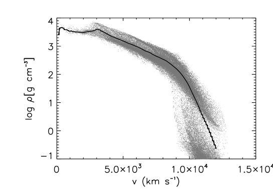
Figure 7: The solid line shows the density distribution with velocity of the spherically averaged 1D model. The grey points each indicate the density and mid-point velocity of a grid cell in the 3D model. All densities are shows for time $t=10$ sec.

We continue to adopt a grey uvoir-absorption cross-section. However, to correctly evaluate the influence of 3D structure on the light curve, it is necessary to consider that compositional inhomogeneity would cause the cross-section per gram to be a function of position. It goes beyond the scope of this paper to undertake full calculations of the composition dependence of the opacity; instead, a simple one-parameter description of the opacity is adopted, following Mazzali & Podsiadolwski (2006). They consider the opacity to be determined by the mass fraction of iron-group elements on the assumption that the opacity per gram is a factor of ten higher for the iron-group than for lighter elements. Adopting the same assumption, the uvoir-absorption cross-section per gram used in this section is given by

$$\sigma=N(0.9X_{\mbox{\scriptsize Fe-grp}}+0.1)\;\;[\mbox{cm${}^{2}$ g${}^{-1}$}]$$ (8)

where $X_{\mbox{\scriptsize Fe-grp}}$ is the mass fraction of iron-group elements, which varies from cell to cell, and the normalisation factor $N$ is chosen such that the mean value of $\sigma$ in the ejecta is fixed to $<\sigma>=0.1$ cm² g^-1. Although crude, this parameterisation captures the essential physics that the heavy elements dominate the mean opacity and only requires the compositional information which is directly available from the explosion model (namely, the total iron-group mass). Note that, for ease of comparison with the constant-$\sigma$ calculations used in the earlier sections of this paper, the time-dependence imposed on $\sigma$ by Mazzali & Podsiadolwski (2006) is not included here.

In view of the simplifications used – in terms of both numerical resolution and particularly the very simple treatment of opacity – the results obtained here should not be regarded as a definitive prediction of the radiation properties of the Röpke et al. (2005) explosion model. Rather, the emphasis is on using a model which has a reliable representation of the degree of inhomogeneity in a real explosion model to understand the role played by the complex structure in the radiation transport.

4.3 uvoir light curves

The light curve obtained with the 3D model described above is shown as the solid histogram in Figure 8; this is the light curve averaged over viewing angles. At peak, this light curve is dimmer than those plotted in Figures 1, 3 and 4; a consequence of the lower ⁵⁶Ni-mass in the present model. The light curve peaks earlier (at $t\approx 13$ days) as a result of differences in the distribution of ⁵⁶Ni with velocity: in the model used here, the ⁵⁶Ni-distribution is less centrally concentrated than that adopted in Sections 2.5 and 3.

To establish the influence of the inhomogeneity on the light curve, the 1D model obtained by spherically averaging the 3D model (see above) was also used to compute a light curve. This light curve is shown by the dashed curve in Figure 8.

From the Figure, it is apparent that the inhomogeneity causes the light curve to be a little brighter at early times and very slightly fainter during the decay phase. This occurs because in the complex 3D medium a fraction of the $r$-packets find trajectories that preferentially pass through lower density cells and therefore encounter lower opacities than is possible in a spherically symmetric model with the same total mass. This allows some $r$-packets to escape more quickly making the light curve brighter during the pre-maximum rise phase. It also means that slightly fewer packets remain trapped in the ejecta which leads to the marginal dimming in the post-maximum phase. The scale of the effect in this model is rather modest: at most it amounts to a difference of $\approx 0.1$ mag and this occurs only at very early times, $\approx 10$ days before maximum light. At around maximum light, the effect is limited to a change in magnitude of around $\Delta M\approx 0.05$ mag (5 per cent in luminosity).

In accordance with “Arnett’s Rule” (Arnett 1982; Arnett, Branch & Wheeler 1985) – which states that the emitted bolometric luminosity is roughly equal to the instantaneous rate of generation of radioactive luminosity at maximum light – the increase in peak luminosity resulting from the 3D structure is accompanied by a faster rise to maximum; the peak luminosity occurs approximately one day earlier in the 3D calculations than the 1D case.

The 3D model was also used to look for viewing-angle dependency of the light curve. Light curves were extracted for a set of eight randomly chosen viewing angles and compared to the angle-averaged light curve. No significant ($>1-2$ per cent) departures from the average light curve were found; this can be understood since large scale departures from sphericity are not present in this model, partially as a result of the assumed reflection symmetries (see above).

It is interesting to note that the results from the model considered here show that inhomogeneity would act in the sense of pushing model results closer to observation; for example, a recent comparison of light curves computed from 1D models with observations (Blinnikov et al. 2006) does suggest that the 1D models produce light curves which rise too slowly and underestimate peak luminosities (see their figures 8 – 13). Direct comparisons with the calculations of Blinnikov et al. (2006) are not possible here owing to the considerably more complex treatment of opacity that they adopt, but it may reasonably be speculated that their rise times would also be shorter if multi-dimensional effects were incorporated.

Figure 8: The light curve obtained from the 3D inhomogeneous model described in Section 4.1 (solid histogram) and the comparison spherically averaged model (dotted line). The light curve computed from the 3D model does not vary significantly with viewing angle.

The scale of the effect here is rather too small to directly have major implications for the confrontation of models and observations. However, the effect is not completely negligible and it is plausible that the calculations presented here may underestimate the true scale of this phenomenon; in particular, both the reduction in resolution from that used in the explosion model and the grossly simplified one-parameter treatment of the opacity may both suppress 3D density and composition effects that would be present in a complete treatment. Furthermore, only one explosion model has been considered here and this model is constructed from a simulation describing only one octant (see above). In the future, it will be necessary to examine a range of models including fully 3D models where the greater complexity may enhance the effects.

5 Discussion

We have described and tested a new 3D, time-dependent Monte Carlo code for modelling radiation transport in SNIa. The code adopts the methods presented by Lucy (2005) and also incorporates a scheme which uses Monte Carlo radiation field estimators to allow observables to be extracted for specific viewing angles; this approach helps to suppress Monte Carlo noise and eliminates the need to obtain intensities by angular binning of emergent Monte Carlo packets.

This code has been used to investigate two classes of three dimensional effects in SNIa models. First, two elliptical SNIa toy models were used to investigate how large scale asphericity might alter observable light curves. As expected from previous simplified treatments (e.g. Höflich 1991), it was found that light curves were brighter when viewed down the minor-axis than the major-axis. The brightness enhancement is largest at early times and becomes smaller during the decline phase as the supernova ejecta becomes less optically thick. For a model with axis ratio comparable to that suggested by polarisation data for real SNIa (Howell et al. 2001; Wang et al. 2003), the differences in peak brightness and light curve shapes between viewing angles is detectable and in principle could play a role in the observed scatter about the mean relationship between light curve brightness and width.

Secondly, a model with structure based on the results of recent three-dimensional hydrodynamical simulations was used to study the effect of inhomogeneities in both density and composition on light curves. It was found that 3D structure could lead to light curves which are both brighter at early times and which peaked sooner after the explosion that is found from 1D models. For the particular model considered, the effect was rather modest ($\approx$ 5 per cent around maximum light) but study of other explosion models is required to quantify the possible diversity in this effect.

Considerable further work is required to fully understand the role of 3D effects on radiation transport in SNIa. The use of the grey approximation in the treatment of uvoir radiation is currently the greatest limiting factor to the practical applicability of these results. In calculations involving a uniform grey absorption coefficient, the line-of-sight opacity depends solely on the total column density. Under realistic conditions for SNIa ejecta, the opacity is dominated by spectral lines (see e.g. Pinto & Eastman 2000b) and is thus a strong function of frequency, velocity gradient, composition and the ionization/excitation state of the plasma. Indeed, when strong lines dominate, the opacity has little direct sensitivity to the column density and is instead mostly a function of the density of spectral lines in frequency space. Furthermore, photon escape from highly opaque material is facilitated by frequency redistribution to those regions of the spectrum where there are relatively few spectral lines (see e.g. Pinto & Eastman 2000b for a detailed discussion); in the grey calculations this means of escape is not available and all the energy packets must burrow through the imposed opacity. Given this, it is likely that the grey approximation overestimates the role of geometry in determining photon propagation. However, further calculations are required to determine and understand this in detail. In the context of the inhomogeneous model discussion in Section 4, a more realistic treatment of the role played by compositional inhomogeneity would be of particular interest; only a crude attempt at describing the variation of opacity with composition has been used here (equation 8) and a sophisticated treatment involving the very real differences between the atomic properties of different elements may lead to interesting effects.

Fortunately, as discussed by Lucy (2005), the Monte Carlo method is well suited to incorporating realistic physics in a complex geometry which will allow the interplay of more detailed micro-physics and 3D structure to be studied in the near future; this would involve a more sophisticated treatment of the opacity, perhaps similar to the methods employed by Blinnikov et al. (2006) or Kasen et al. (2006). From such a calculations it would be possible to extract not only a bolometric light curve, but also light curves for specific photometric bands, an important step in the progression towards confrontation of theory and observation.

Light curve calculations also need to be performed for a wider range of explosion models than the exploratory set discussed here. This is necessary in order to quantify how the various effects might differ in scale depending on various properties of the explosion and so help to understand what role they might play in establishing both the average properties and diversity of SN observations.

Eventually, it would also be valuable to undertake a similar assessment of the role of 3D effects in full NLTE modelling of uvoir-spectra; much of the greatest diagnostic power lies in spectral modelling – including both intensity and polarimetry – and thus it is important that commonly used modelling assumptions, such as that of spherical symmetry, are studied in the context of modern explosion models.

References

Arnett W. D., 1982, ApJ, 253, 785
Arnett W. D., Branch D., Wheeler J. C., 1985, Nature, 314,
337
Ambwani K., Sutherland P., 1988, ApJ, 325, 820
Benetti S., et al., 2004, MNRAS, 348, 261
Benetti S., et al., 2005, ApJ, 623, 1011
Blinnikov S. I., Röpke F. K., Sorokina E. I., Gieseler M.,
Reinecke M., Travaglio C., Hillebrandt W., Stritzinger
M., 2006, A&A, 453, 229
Branch D., Falk S. W., Uomoto A. K., Wills B. J., McCall
M. L., Rybski P., 1981, ApJ, 244, 780
Branch D, 1992, ApJ, 392, 35
Gamezo V. N., Khokhlov A. M., Oran E. S., Chtchelkanova
A. Y., Rosenberg R. O., 2003, Science, 299, 77
Höflich P., 1991, A&A, 246, 481
Höflich P., Wheeler J. C., Thielemann F. K., 1998, ApJ,
495, 617
Howell D. A., Höflich P., Wang L., Wheeler J. C., 2001,
ApJ, 556, 302
Hoyle F., Fowler W. A., 1960, ApJ, 132, 565
Kasen D., Thomas R. C., Nugent P., 2006, ApJ, 651, 366
Kozma C., Fransson C., Hillebrandt W., Travaglio C.,
Sollerman J., Reinecke M., Röpke F. K., Spyromilio J.,
2005, A&A, 437, 983
Lucy L. B., 1999, A&A, 345, 211
Lucy L. B., 1987, in ESO Workshop on the SN 1987A, ed.
I. J. Danziger, 417, European Southern Observatory,
Garching
Lucy L. B., 2005, A&A, 429, 19
Maeda K., Mazzali P. A., Nomoto K., 2006, ApJ, 645, 1331
Mazzali P. A., Lucy L. B., 1993, A&A, 279, 447
Mazzali P. A., Podsiadlowski Ph., 2006, MNRAS, 369, L19
Niemeyer J. C., Hillebrandt W., Woosley S. E., 1996, ApJ,
471, 903
Nomoto K., Thielemann F.-K., Yokoi K., 1984, ApJ, 286,
644
Müller E., Arnett W. D., 1986, ApJ, 307, 619
Phillips M. M., 1993, ApJ, 413, L105
Pinto P. A., Eastman R. G., 2000a, ApJ, 530, 744
Pinto P. A., Eastman R. G., 2000b, ApJ, 530, 757
Reinecke M., Hillebrandt W., Niemeyer J. C., 2002, A&A,
391, 1167
Röpke F. K., 2005, A&A, 432, 969
Röpke F. K., Gieseler M., Reinecke M., Travaglio C.,
Hillebrandt W., 2006, A&A, 453, 203
Wang L., et al. 2003, ApJ, 591, 1110
Yoon S.-C., Langer N., 2005, A&A, 435, 967