Vertex renormalization in weak decays of Cooper pairs and cooling compact stars

Abstract

At temperatures below the critical temperature of superfluid phase transition baryonic matter emits neutrinos by breaking and recombination of Cooper pairs formed in the condensate. The strong interactions in the nuclear medium modify the weak interaction vertices and the associated neutrino loss rates. We study these modifications non-perturbatively by summing infinite series of particle-hole loops in the $S$-wave superfluid neutron matter. The pairing and particle-hole interactions in neutron matter are described in the framework of the BCS and Fermi-liquid theories derived from microscopic interactions. Consistent with the $f$-sum rule, the leading order contribution to the polarization tensor arises at $O(q^{2})$ in the small momentum transfer, $q$, expansion. The associated neutrino emission rate is parametrically suppressed compared to its one-loop counterpart by a factor of the order of $5\times 10^{-3}$, the parameter being the baryon recoil in units of temperature.

I Introduction

Pair-correlated baryonic matter in compact stars emits neutrinos via the weak neutral current processes of pair-breaking and recombination FRS78 ; VS87+MIGDAL90

$$\{NN\}\to N+N+\nu_{f}+\bar{\nu}_{f},\quad N+N\to\{NN\}+\nu_{f}+\bar{\nu}_{f},$$ (1)

where $\{NN\}$ refers to a Cooper pair, $N+N$ to two quasiparticle excitations, $\nu_{f}$ and $\bar{\nu}_{f}$ to the neutrino and anti-neutrino of flavor $f$. The process (1) is limited to the temperature domain $T^{*}\leq T\leq T_{c}$, where $T_{c}$ is the critical temperature of pairing phase transition and $T^{*}\sim 0.2~{}T_{c}$. At and above $T_{c}$ this reaction cannot occur, since momentum and energy cannot be conserved simultaneously in a process $N\to N+\nu_{f}+\bar{\nu}_{f}$, i. e., an on-mass-shell fermion cannot produce bremsstrahlung (in the absence of external gauge fields). At asymptotically low temperatures, $T\leq T^{*}$, the rate of the process (1) is exponentially small since the number of excitations out of the condensate is suppressed as ${\rm exp}(-\Delta/T)$, where $\Delta(T)$ is the gap in the quasiparticle spectrum.

Cooling simulations of neutron stars revealed the efficiency of the processes (1) in refrigerating the baryonic interiors of a compact star from temperatures $T\leq T_{c}\sim 10^{9}$ K down to temperatures of the order of $10^{8}$ K SCHAAB96 ; TSU ; GRIG ; PAGE_MINIMAL . The temperature domain above corresponds to the neutrino cooling era that spans the time domain $10^{2}\leq t\leq 10^{5}$ years. The predicted surface temperatures of neutron stars during this and the following photon cooling era (where the star loses its thermal energy by emission of photons from the surface) are sensitive to the neutrino emission rates within this time-domain. Remarkably, the process (1) relates the cooling rate of a compact star to the microscopic physics of its interiors and is particularly sensitive to the density-temperature phase diagram of paired baryonic matter. Therefore, the measurements of the surface (photon) luminosities of neutron stars and their interpretation in terms of cooling simulations have predictive power for analyzing the phase diagram and composition of baryonic matter GRIG_VOSK ; KHODEL ; VOSK_REVIEW ; SEDRAKIAN_REVIEW .

The rate of the process (1) was computed independently (and within alternative methods) in Refs. FRS78 ; VS87+MIGDAL90 in the case where the pairing interaction is in the ${}^{1}S_{0}$ partial wave, i. e., nucleons are paired in a spin-0, isospin-1 state, (the influence of electric charge carried by proton Cooper pairs and the case of pairs forming a spin 1-superfluid are discussed in Refs. 1LOOP ). In propagator language these rates correspond to the one-loop approximation to the polarization tensor of baryonic matter VS87+MIGDAL90 ; SEDRAKIAN_REVIEW . It has been known for a long time that the gauge invariance requires summation of infinite series of loop diagrams (known as RPA resummation) in conventional superconductors NAMBU ; SCHRIEFFER . Ref. KUNDU_REDDY carried out RPA summations in neutron and quark matter within the context and kinematics of neutrino scattering in hot proto-neutron stars. Subsequently, Ref. LP applied the gauge invariance and vertices derived by Nambu NAMBU to the neutrino emission processes in the vector channel and concluded that the rates are suppressed by by many order of magnitude.

We shall arrive below at results which are at variance to those of Ref. LP for the following reasons. The effective vertices implemented in Ref. LP were derived within a zero-temperature theory NAMBU ; herein we shall derive the vertices at finite temperature, consistent with the polarization tensor of matter. This guarantees that the unitarity of the $S$-matrix in the quantum mechanical process of the bremsstrahlung is preserved. Second, while in Ref. LP the matrix elements are expanded in the parameter $v_{F}/c$, where $v_{F}$ is the baryon velocity, and the leading order contribution to the rates comes from the terms $O(v_{F}/c)^{4}$, herein the polarization tensor is expanded in small momentum transfer, $q$; the leading order contribution to the rates arises at $O(q^{2})$ consistent with the $f$-sum rule. As a consequence, we find a suppression of the neutrino bremsstrahlung rate which is by several orders of magnitude less than predicted in Ref. LP . Since the magnitude of the pairing gaps are not well known and the neutrino bremsstrahlung rates are rather sensitive to the value of the gap, the pairing braking process in $S$-wave superfluids remains a potentially viable mechanism of cooling of neutron stars.

We start by setting up a formalism for computing the vertex corrections to weak reaction rates that arise due to the strong interactions in baryonic matter. We consider the case of neutron matter at subnuclear densities, which we describe within the Landau Fermi-liquid theory derived from microscopic interactions. At these densities neutron matter is characterized by an isotropic order parameter arising form the interaction in the ${}^{1}S_{0}$ partial wave channel; we solve the corresponding problem of pairing in the framework of the Bardeen-Cooper-Schrieffer (BCS) theory. In the non-relativistic limit, the vector and axial vector weak vertices are associated with scalar and spinor perturbations. Thus, the problem of the weak vertex renormalization reduces to a study of the effective three-point vertices that sum-up particle-hole irreduceable ladders in superfluid matter in the scalar and spin channels. In a wider context, such resummations describe of the low-frequency, long-wave-length collective modes of superfluid Fermi-liquids SCHRIEFFER ; LEGGET ; MIGDAL . In particlar, such resummations, known as quasiparticle random phase approximation (QRPA), have been widely used in nuclear structure calculations RING_SCHUCK .

The paper is organized as follows. Section II introduces the Green’s functions formalism and computes, for the sake of illustration, the neutrino rates at one-loop. In Sec. III the modifications of the weak interaction vertices are computed by summing particle-hole ladders in superfluid neutron matter. Section IV is devoted to the computation of the full polarization tensor that includes the vertex corrections derived in the preceding Section. Section V contains our conclusion. Some technical details are relegated to the Appendix.

II $S$-wave pair-condensation in neutron matter

Below we shall describe the neutron pair-condensate at subnuclear densities within the framework of the Fermi-liquid theory, which assumes that the elementary degrees of freedom are quasiparticles with well defined momentum-energy relation and infinite life-time. The interactions between the quasiparticles are then described in terms of Landau parameters which depend on the momentum transfer (or scattering angle). Since the scattering angles involved are typically small, the momentum dependence of Landau parameters is further approximated by the leading and next-to-leading order terms in the expansion in Legendre polynomial with respect to the scattering angle. The problem of pairing in neutron matter will be solved below within the BCS approximation, where the anomalous self-energy (the gap function) is computed from the bare interaction while the normal self-energy is computed within the decoupling approximation which ignores the effects of pair-correlations on the single particle spectrum of quasiparticles. A number of factors such as the renormalization of the pairing interaction PETHICK ; CLARK76 ; CHEN86 ; CHEN93 ; WAMBACH ; SCHULZE96 ; SEDRAKIAN03 ; SCHWENK ; LOMB1 ; FABROCINI and the wave-function renormalization SEDRAKIAN03 ; LOMB2 ; MUDICK , affect the absolute value of the gap. The role of these factors has not been settled yet, and we shall employ below the standard BCS approach which has led to convergent and verifiable results for neutron matter (see the reviews REVIEW1 ; REVIEW2 ; REVIEW3 ).

Since the baryonic component of stellar matter is in thermal equilibrium to a good approximation, we shall adopt the Matsubara Green’s functions for the description of the neutron condensate and for the evaluation of the polarization tensor. In the case of ${}^{1}S_{0}$ pairing these are defined as (e. g. Ref. ABRIKOSOV , pg. 120)

$$\hat{G}_{\alpha\alpha^{\prime}}(\bm{p},\tau) = -\delta_{\alpha\alpha^{\prime}}\langle T_{\tau}a_{p\alpha}(\tau)a^{\dagger}_{p\alpha^{\prime}}(0)\rangle,$$ (2)

$$\hat{F}_{\alpha\alpha^{\prime}}(\bm{p},\tau) = \delta_{\varsigma\varsigma^{\prime}}\langle T_{\tau}a_{-p\downarrow}(\tau)a_{p\uparrow}(0)\rangle,$$ (3)

$$\hat{F}^{\dagger}_{\alpha\alpha^{\prime}}(\bm{p},\tau) = \delta_{\varsigma\varsigma^{\prime}}\langle T_{\tau}a_{p\uparrow}^{\dagger}(\tau)a^{\dagger}_{-p\downarrow}(0)\rangle,$$ (4)

where $\alpha$ stands for spin $\sigma=\uparrow,\downarrow$ and isospin $\varsigma$, $\tau$ is the imaginary time, $T_{\tau}$ is the imaginary time ordering symbol, $a^{\dagger}_{p\sigma}(\tau)$ and $a_{p\sigma}(\tau)$ are the creation and destruction operators. In the momentum representation the propagators are given by

$$\hat{G}_{\alpha\alpha^{\prime}}(ip_{n},\bm{p}) = \delta_{\sigma\sigma^{\prime}}\delta{\varsigma\varsigma^{\prime}}\left(\frac{u_{p}^{2}}{ip_{n}-\epsilon_{p}}+\frac{v_{p}^{2}}{ip_{n}+\epsilon_{p}}\right),$$ (5)

$$\hat{F}_{\alpha\alpha^{\prime}}(ip_{n},\bm{p}) = -i\sigma_{y}\delta{\varsigma\varsigma^{\prime}}u_{p}v_{p}\left(\frac{1}{ip_{n}-\epsilon_{p}}-\frac{1}{ip_{n}+\epsilon_{p}}\right),$$ (6)

and $F_{\alpha\alpha^{\prime}}^{\dagger}(ip_{n},\bm{p})=F_{\alpha\alpha^{\prime}}(ip_{n},\bm{p})$, where $p_{n}=(2n+1)\pi T$ is the fermionic Matsubara frequency, $\sigma_{y}$ is the $y$-component of the Pauli-matrix, $u_{p}^{2}=(1/2)(1+\xi_{p}/\epsilon_{p})$ and $v_{p}^{2}=1-u_{p}^{2}$ are the Bogolyubov amplitudes and

$$\epsilon_{p}=\sqrt{\xi_{p}^{2}+\Delta_{p}^{2}}$$ (7)

is the quasiparticle spectrum, where $\xi_{p}=p^{2}/2m+{\rm Re}\Sigma(p)-\mu$ is the spectrum in the unpaired state with $m$ and $\mu$ being the bare mass and chemical potential. Here $\Sigma(p)$ and $\Delta(p)$ are the normal and anomalous self-energies. For the later diagrammatic analysis we shall need the hole propagator which is given by

$$\hat{G}_{\alpha\alpha^{\prime}}^{\dagger}(ip_{n},\bm{p}) = \hat{G}_{\alpha\alpha^{\prime}}(-ip_{n},-\bm{p})$$ (8)

$$= -\delta_{\sigma\sigma^{\prime}}\delta{\varsigma\varsigma^{\prime}}\left(\frac{u_{p}^{2}}{ip_{n}+\epsilon_{p}}+\frac{v_{p}^{2}}{ip_{n}-\epsilon_{p}}\right).$$

The spin and isospin dependence of propagators for $S$-wave spin-0 and isospin-1 pairing is: $\hat{G}_{\alpha\alpha^{\prime}}(ip_{n},\bm{p})=\delta_{\sigma\sigma^{\prime}}\delta{\varsigma\varsigma^{\prime}}G(ip_{n},\bm{p})$ and $\hat{F}_{\alpha\alpha^{\prime}}(ip_{n},\bm{p})=-i\sigma_{y}\delta{\varsigma\varsigma^{\prime}}F(ip_{n},\bm{p})$.

Since the quasiparticles are confined to the vicinity of the Fermi-surface we expand the normal self-energy around the Fermi momentum, $p_{F}$, to obtain

$$\epsilon(p)=\frac{p_{F}}{m^{*}}(p-p_{F})-\mu^{*}\,,$$ (9)

$$\frac{m^{*}}{m}=\left[1+\frac{m}{p_{F}}\partial_{p}{\rm Re}\Sigma(p)|_{p=p_{F}}\right]^{-1}\,,$$ (10)

where $\mu^{*}\equiv-\epsilon(p_{F})+\mu-{\rm Re}\Sigma(p_{F})$ is the effective chemical potential, $m^{*}$ is the effective mass. The dependence of the self-energies on the off-mass shell energy will be neglected, i. e. the wave-function renormalization which accounts for the next-to-leading term in the expansion around the Fermi-energy is set to unity.

Figure 1: Temperature dependence of the ${}^{1}S_{0}$ pairing gap in neutron matter for Fermi wave vectors $p_{F}=0.4$ (solid line), $0.8$ (dashed line), 1.2 (dashed-dotted line) and 1.6 (dashed-double-dotted line).

The BCS mean-field approximation to the anomalous self-energy can be written in terms of the attractive four-point vertex function $\Gamma(p,p^{\prime})$ in the form

$$\Delta(p)=-2\int\!\frac{d^{4}p^{\prime}}{(2\pi)^{4}}\Gamma(p,p^{\prime})~{}{\rm Im}F(p^{\prime})f(\omega^{\prime})\,,$$ (11)

where $f(\omega)=[1+{\rm exp}(\beta\omega)]^{-1}$ is the Fermi distribution function and $\beta$ is the inverse temperature. For the problem of neutron matter at subnuclear densities we adopt the standard BCS approach and thus approximate the four-point vertex by the bare interaction in the ${}^{1}S_{0}$ partial wave channel and the single particle spectrum by the on-shell spectrum given by Eq. (9).

Table 1: Density dependence of the effective mass, the scalar and spin-spin interactions, the pairing gap and the critical temperature; the interactions are given in units of the density of states $\nu(p_{F})$.

$p_{F}$	$m^{*}/m$	$v^{V}$	$v^{A}$	$\Delta(p_{F})$	$T_{c}$
[fm-1]				[MeV]	[MeV]
0.4	1.02	-0.56	0.55	1.54	0.85
0.6	1.00	-0.50	0.49	2.60	1.44
0.8	0.97	-0.47	0.44	3.15	1.78
1.0	0.94	-0.45	0.41	3.09	1.80
1.2	0.92	-0.43	0.40	2.44	1.46
1.4	0.88	-0.41	0.40	1.41	0.88
1.6	0.84	-0.36	0.39	0.57	0.38

With these approximation Eq. (11) reduces to

$$\Delta(p)=\int\!\frac{d^{3}p^{\prime}}{2(2\pi)^{3}}V(p,p^{\prime})\frac{\Delta(p^{\prime})}{\sqrt{\xi(p^{\prime})^{2}+\Delta(p^{\prime})^{2}}}\left[1-2f(\epsilon(p^{\prime}))\right]\,.$$ (12)

The gap equation is supplemented by the equation for the density of the system,

$$\rho=-2\int\!\!\frac{d^{4}p}{(2\pi)^{4}}{\rm Im}G(p)f(\omega),$$ (13)

which determines the chemical potential in a self-consistent manner. Fig. 1 shows the temperature dependence of the ${}^{1}S_{0}$ pairing gap in neutron matter for several densities parameterized in terms of the Fermi wave number, $\rho=p_{F}^{3}/3\pi^{2}$. The gap at zero temperature and the critical temperature for unpairing are listed in the Table 1. The dependence of ratio $\Delta(T)/T$ on $T/T_{c}$ in this model is non-universal, i. e. it depends on the density; this is contrary to the prediction of the BCS theory with contact pairing interaction.

Within the adopted Fermi-liquid description of neutron matter, the particle-hole interaction is given by

$$V^{ph}(\bm{q})=v^{V}(\bm{q})+v^{A}(\bm{q})({\bm{\sigma}}\cdot{\bm{\sigma}}^{\prime}),$$ (14)

where ${\bm{\sigma}}$ refers to the Pauli matrix. The Landau parameters $v^{V}(\bm{q})$ and $v^{A}(\bm{q})$ depend on the momentum transfer $\bm{q}$ in the process where both fermion momenta are on the Fermi-surface NOTE1 . The tensor and spin-orbit terms are small in neutron matter and were neglected in Eq. (14). The full dependence of these parameters on the momentum transfer is commonly approximated by a Legendre polynomial with respect to the angle formed by the incoming fermions, whereby only the leading and next-to-leading order terms contribute significantly.

Table 1 lists the effective mass, the zeroth order Landau parameters in the scalar and spin channels computed within the formalism of Ref. DICKHOFF starting from the CD Bonn potential MACHLEIDT . The solution of the gap equation was obtained by applying the iterative method with “running” cut-off SC06 whereby the effective pairing interaction was approximated by the Gogny DS1 force SKMS .

III The pair-breaking processes at one-loop

The neutrino emissivity (the power of the energy radiated per unit volume in neutrino-anti-neutrino pairs) is given by VS87+MIGDAL90 ; SEDRAKIAN_DIEPERINK

$$\epsilon_{\nu\bar{\nu}} = -2\left(\frac{G}{2\sqrt{2}}\right)^{2}\int\!\frac{d^{3}q_{1}}{(2\pi)^{3}2\omega_{1}}\int\!\frac{d^{3}q_{2}}{(2\pi)^{3}2\omega_{2}}\int\!dq_{0}$$ (15)

$$\times \int\!d^{3}\bm{q}\,\delta(\bm{q}_{1}+\bm{q}_{2}-\bm{q})\delta(\omega_{1}+\omega_{2}-q_{0})\,q_{0}$$

$$\times g(q_{0})\Lambda^{\mu\zeta}(q_{1},q_{2})\Im{\rm m}\,\Pi_{\mu\zeta}(q),$$

where $G$ is the weak coupling constant, $q_{i}=(\omega_{i},\bm{q}_{i})$, $i=1,2$ are the on-mass-shell four-momenta of neutrinos, $g(q_{0})=[{\rm exp}(q_{0}/T)-1]^{-1}$ is the Bose distribution function, $\Pi_{\mu\zeta}(q)$ is the retarded polarization tensor, $\Lambda^{\mu\lambda}(q_{1},q_{2})={\rm Tr}\left[\gamma^{\mu}(1-\gamma^{5})\!\not\!q_{1}\gamma^{\nu}(1-\gamma^{5})\!\not\!q_{2}\right]$. Here and below the emissivities are given per neutrino flavor; the total rate is obtained upon multiplying the single flavor rate by the number of neutrino flavors within the standard model, $N_{f}=3$. The polarization tensor of baryons at one-loop is shown in Fig. 2 and is given analytically by

$$\Pi^{V/A}(q)=T\sum_{\sigma,p}\left[G(p)G(p+q)\mp F(p)F^{\dagger}(p+q)\right],$$ (16)

where $p=(ip_{0},\bm{p})$. The upper/lower signs correspond to vector current ($V$) and axial vector current ($A$) couplings. In writing Eq. (16) we assumed that baryons carry the same isospin quantum number.

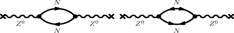
Figure 2: The one-loop contribution to the polarization tensor in the superfluid matter; solid lines refer to the baryon propagators, wavy lines to the (amputated) $Z^{0}$ propagator.

Performing the Matsubara sums in Eq. (16) (see the Appendix) we obtain

$$\Pi^{V/A}(q) = \sum_{\sigma\bm{p}}\left[f(\epsilon_{p})-f(\epsilon_{k})\right]\left(\frac{A_{\mp}}{iq+\epsilon_{p}-\epsilon_{k}}-\frac{B_{\mp}}{iq-\epsilon_{p}+\epsilon_{k}}\right)$$ (17)

$$+ \sum_{\sigma\bm{p}}\left[f(-\epsilon_{p})-f(\epsilon_{k})\right]\left(\frac{C_{\mp}}{iq-\epsilon_{k}-\epsilon_{p}}-\frac{D_{\mp}}{iq+\epsilon_{p}+\epsilon_{k}}\right),$$

where $k=p+q$, $A_{\mp}=u_{p}^{2}u_{k}^{2}\mp h$, $B_{\mp}=v_{p}^{2}v_{k}^{2}\mp h$, $C_{\mp}=u_{k}^{2}v_{p}^{2}\pm h$, $D_{\mp}=u_{p}^{2}v_{k}^{2}\pm h$, $h=u_{p}u_{k}v_{p}v_{k}$. The emissivity (15) requires the imaginary part of the polarization tensor which after analytical continuation in Eq. (17) becomes [note that $f(-\epsilon_{p})=1-f(\epsilon_{p})]$

$$\Im{\rm m}\,\Pi^{V/A}(q) = -\pi\sum_{\sigma\bm{p}}\left[f(\epsilon_{p})-f(\epsilon_{k})\right](A_{\mp}+B_{\mp})~{}\delta(\omega+\epsilon_{p}-\epsilon_{k})$$ (18)

$$- \pi\sum_{\sigma\bm{p}}\left[f(-\epsilon_{p})-f(\epsilon_{k})\right]\left[C_{\mp}~{}\delta(\omega-\epsilon_{p}-\epsilon_{k})-D_{\mp}~{}\delta(\omega+\epsilon_{p}+\epsilon_{k})\right].$$

To obtain the first line we used the fact that the quasiparticle spectra are invariant under spatial reflections, i. e., $\epsilon(-\bm{p})=\epsilon(\bm{p})$. The first line in Eq. (18) corresponds to the process of scattering where a quasiparticle is promoted out of the condensate into an excited state, or inversely, an excitation merges with the condensate. The corresponding piece of the response function $\Im{\rm m}\Pi^{V/A}(q)$ vanishes for small momentum transfers. Indeed neutrino energies are of the order of temperature which implies that their wave vectors $q[{\rm fm}^{-1}]\sim\omega_{\nu}/\hbar c\sim T/\hbar c\sim 1/197.3\ll 1$. On the other hand the neutron wave vectors $p\sim p_{F}\sim 1$ fm^-1. Upon expanding the argument of the delta-function with respect to $|q|$ around the point $q=0$ one finds

$$\omega-q\,\frac{\xi_{p}}{\epsilon_{p}}\frac{\partial\xi_{p+q}}{\partial q}\Big{|}_{q=0}-q\,\frac{\Delta_{p}}{\epsilon_{p}}\frac{\partial\Delta_{p+q}}{\partial q}\Big{|}_{q=0}=0.$$ (19)

If we assume that $\Delta\neq\Delta(p)$ the third term on the l. h. side vanishes. It follows that $x\equiv(\bm{p}\cdot\bm{q})/pq=(\epsilon_{p}/\xi_{p})(\omega/vq)\leq 1$, where $v~{}(\sim v_{F})$ is the baryon (Fermi) velocity. For on mass-shell neutrinos $\omega=cq$ and the latter condition can not be satisfied, i. e. the scattering contribution can be neglected. The non-locality in the momentum or frequency domains of the gap function will alter this conclusion, but will require a specific model of the momentum and frequency dependence of the gap function (for $S$-wave interactions the momentum and energy dependences are described respectively in Refs. LOMB3 ; SKMS ; KUCKEI ; MUDICK and LOMB1 ; SEDRAKIAN03 ; LOMB2 ). The second line in Eq. (18) describes the process of pair-breaking and recombination, i. e., excitation of pairs of quasiparticles out of the condensate, and inversely, restoration of a pair within the condensate. Since we are interested in the emission process we shall keep only the terms that do not vanish for $\omega>0$; then, the pair-braking contribution is given by

$$\Im{\rm m}\,\Pi^{V/A}(q)=-\pi\sum_{\sigma\bm{p}}\left[f(-\epsilon_{p})-f(\epsilon_{k})\right]C_{\mp}.$$ (20)

In the limit $\bm{q}\to 0$ and assuming that $\Delta\neq\Delta(p)$ the integrations in Eq. (20) can be performed analytically. One finds

$$\Im{\rm m}\,\Pi^{V}(q) = -2\pi\nu(p_{F})g(\omega)^{-1}f\left(\frac{\omega}{2}\right)^{2}\left(\frac{\Delta^{2}}{\omega^{2}}\right)\frac{\omega}{\sqrt{\omega^{2}-4\Delta^{2}}}\theta(\omega-2\Delta),$$ (21)

$$\Im{\rm m}\,\Pi^{A}(q) \simeq 0+O\left(\frac{v_{F}^{2}}{c^{2}}\right),$$ (22)

where $\nu(p_{F})=m^{*}p_{F}/2\pi^{2}$ is the density of states ($\hbar=1$) and $\theta$ is the Heaviside step function; the explicit form of the $O\left({v_{F}^{2}}/{c^{2}}\right)$ contribution to the axial current response is given in Ref. FRS78 . Note the threshold behavior of the vector current response, which is finite for frequencies that are large compared to $2\Delta$ - the energy needed to break a pair.

Upon substituting Eq. (21) in Eq. (15) and carrying out the phase-space integrals we obtain the emissivity per neutrino flavor FRS78 ; VS87+MIGDAL90

$$\epsilon^{\rm 1-loop}_{\nu\bar{\nu}}=\epsilon_{0}~{}z^{2}~{}\int_{2z}^{\infty}\!\!dx\frac{x^{5}}{\sqrt{x^{2}-4z^{2}}}~{}f\left(\frac{x}{2}\right)^{2}$$ (23)

where $z=\Delta(T)/T$ and

$$\epsilon_{0}=\frac{\nu(p_{F})G^{2}c_{V}^{2}}{60~{}\pi^{3}}T^{7}.$$ (24)

IV Weak interaction vertices

Figure 3: Coupled integral equations for the effective weak vertices in superfluid baryonic matter. The “normal” $\Gamma_{1}$ vertex (full triangle) and two “anomalous” vertices $\Gamma_{2}$ (hatched) and $\Gamma_{3}$ (shaded triangle) are shown explicitly, the fourth vertex (empty triangle) is obtained by interchanging the particle and hole lines in the first line. The anomalous vertices vanish in the normal state.

Consider the weak vector and axial vector vertices in the nuclear medium featuring a condensate. Because the particle-hole interactions in the medium (which are represented by the Landau parameters in Table 1) are not small, the vertex renormalization requires a summation of an infinite number of particle-hole loops. There are four topologically non-equivalent vertices in the superfluid state in general, but, as we shall see, the particle-hole symmetry reduces their number by one. Since neutrons pair in an isospin-1 state (neutron-proton pairing is unimportant for large asymmetries ASYM ) we shall suppress the isospin indices. The expansion of the Landau parameters in Legendre polynomials will be truncated at the leading order (the next-to-leading order terms are suppressed by powers of $v_{F}/c$). Thus, the effective particle-hole interaction is given by

$$v=v^{V}+v^{A}({\bm{\sigma}}\cdot{\bm{\sigma}}^{\prime}).$$ (25)

The integral equation defining the effective weak vertices, which we write in an operator form, are given by

$$\hat{\Gamma}_{1}^{a} = \Gamma_{0}^{a}+v^{a}(G\Gamma_{1}^{a}G+\hat{F}\Gamma_{3}^{a}G+G\Gamma_{2}^{a}\hat{F}+\hat{F}\Gamma_{4}^{a}\hat{F}),$$ (26)

$$\hat{\Gamma}_{2}^{a} = \quad\quad v^{a}(G\Gamma_{2}^{a}G^{\dagger}+\hat{F}\Gamma_{4}^{a}G^{\dagger}+G\Gamma_{1}^{a}\hat{F}+\hat{F}\Gamma_{3}^{a}\hat{F}),$$ (27)

$$\hat{\Gamma}_{3}^{a} = \quad\quad v^{a}(G^{\dagger}\Gamma_{3}^{a}G+\hat{F}\Gamma_{1}^{a}G+G^{\dagger}\Gamma_{4}^{a}\hat{F}+\hat{F}\Gamma_{2}^{a}\hat{F}),$$ (28)

and are displayed diagrammatically in Fig. 3. Here $\hat{F}=-i\sigma_{y}F$, $v^{a}$ with $a\in V,A$ are defined in Eq. (25), while $\Gamma_{0}^{V}=1$ and $\Gamma_{0}^{A}={\bm{\sigma}}$. The fourth integral equation for the vertex $\Gamma_{4}^{a}$ follows upon interchanging in Eq. (26) particle and hole propagators $G\leftrightarrow G^{\dagger}$. The momentum space representation of Eq. (26) reads

$$\hat{\Gamma}_{1}^{a}(q)=\Gamma_{0}^{a} + v^{a}\int\frac{d^{4}p}{(2\pi)^{4}}\Bigr{[}G(p)\Gamma_{1}^{a}(q)G(p+q)+G(p)\Gamma_{2}^{a}(q)\hat{F}(p+q)$$ (29)

$$+ F\hat{(}p)\Gamma_{3}^{a}(q)G(p+q)+\hat{F}(p)\Gamma_{4}^{a}(q)\hat{F}(p+q)\Bigl{]},$$

with similar expressions for Eqs. (27) and (28). Even though the driving interactions are local in time, the resummations at finite temperatures lead to time-retarded interactions, which imply that the effective vertices in Eqs. (26)-(28) are complex in general. Considering the scalar interaction $\Gamma_{0}^{V}$ we obtain

$$v^{V}\left(\begin{array}[]{ccc}(v^{V})^{-1}-[\Pi_{GG}(q)-\Pi_{FF}(q)]&\Pi_{GF}(q)&\Pi_{FG}(q)\\ -2\Pi_{GF}(q)&(v^{V})^{-1}-\Pi_{GG\dagger}(q)&\Pi_{FF}(q)\\ -2\Pi_{FG}(q)&\Pi_{FF}(q)&(v^{V})^{-1}-\Pi_{G\dagger G}(q)\end{array}\right)\left(\begin{array}[]{c}\Gamma^{V}_{1}(q)\\ \Gamma^{V}_{2}(q)\\ \Gamma^{V}_{3}(q)\end{array}\right)=\left(\begin{array}[]{c}\Gamma^{V}_{0}\\ 0\\ 0\end{array}\right),$$ (30)

where, using the abbreviations $X,X^{\prime}\in G,F,G^{\dagger}$, we defined (see the Appendix)

$$\Pi_{XX^{\prime}}(q)=\int\frac{d^{3}\bm{p}}{(2\pi)^{3}}L_{XX^{\prime}}(q,\bm{p})=\int\frac{d^{3}\bm{p}}{(2\pi)^{3}}\sum_{ip}X(p)X^{\prime}(p+q).$$ (31)

The loop integrals posses the following symmetries: $L_{GG}=L_{G^{\dagger}G^{\dagger}}$, $L_{GF}=L_{FG^{\dagger}}$ and $L_{FG}=L_{G^{\dagger}F}$, which imply that $\Gamma_{1}^{V}=\Gamma_{4}^{V}$ and $\Gamma_{1}^{A}=-\Gamma_{4}^{A}$. For energy-momentum independent interactions the integral equation (30) reduces to three coupled linear equation for the complex functions $\Gamma^{V}_{i}$, $i=1,2,3$. The details of the computation of the coefficients in Eqs. (30) are relegated to the Appendix.

In the case of axial-vector interactions the effective vertices are given by

$$v^{A}\left(\begin{array}[]{ccc}(v^{A})^{-1}&\Pi_{GF}(q)&\Pi_{FG}(q)\\ 0&(v^{A})^{-1}-\Pi_{GG\dagger}(q)&\Pi_{FF}(q)\\ 0&\Pi_{FF}(q)&(v^{A})^{-1}-\Pi_{G\dagger G}(q)\end{array}\right)\left(\begin{array}[]{c}\Gamma^{A}_{1}(q)\\ \Gamma^{A}_{2}(q)\\ \Gamma^{A}_{3}(q)\end{array}\right)=\left(\begin{array}[]{c}\Gamma^{A}_{0}\\ 0\\ 0\end{array}\right).$$ (32)

This equation has a “trivial” solution $\Gamma^{A}_{1}=1$ and $\Gamma^{A}_{2}=\Gamma^{A}_{3}=0$ to the leading order in the $v_{F}^{2}/c^{2}$ expansion and we shall not consider it further. In the weak-coupling BCS limit there exist approximate constraints among the loop integrals

$$L_{GF}=-L_{FG},\quad\quad L_{G^{\dagger}G}=L_{GG^{\dagger}},$$ (33)

which allow us to reduce the number of equations in the set (30) from three to two. The relations (33) are exact at the threshold $\omega=2\Delta$ and hold approximately for systems with strong degeneracy (corrections being suppressed by powers of the ratio of the temperature over the Fermi-energy). It follows then from Eq. (30) that $\Gamma_{2}^{V}=-\Gamma_{3}^{V}$. The solutions for the remaining vertices $\Gamma_{1}$ and $\Gamma_{2}$ are convenient to express through linear combinations of the polarization tensors (31), defined as

$${\cal A}(q) = \Pi_{GG}(q)-\Pi_{FF}(q)=\int\!\!\frac{d^{3}p}{(2\pi)^{3}}{\cal F}_{p}^{-}(\bm{q}){\cal L}_{p}(\omega,\bm{q}),$$ (34)

$${\cal B}(q) = 2\Pi_{FG}(q)=-\omega\Delta\int\!\!\frac{d^{3}p}{(2\pi)^{3}}\frac{{\cal L}_{p}(\omega,\bm{q})}{\epsilon_{p}},$$ (35)

$${\cal C}(q) = \Pi_{GG^{\dagger}}(q)+\Pi_{FF}(q)-(v^{V})^{-1}=\int\!\!\frac{d^{3}p}{(2\pi)^{3}}\left[2\epsilon_{p}{\cal L}_{p}(0,0)-{\cal F}_{p}^{+}(\bm{q}){\cal L}_{p}(\omega,\bm{q})\right],$$ (36)

where ($\bm{k}=\bm{p}+\bm{q}$)

$${\cal F}_{p}^{\pm}(\bm{q}) = \left(\frac{\epsilon_{p}+\epsilon_{k}}{2}\right)\left(1\pm\frac{\xi_{p}\xi_{k}}{\epsilon_{p}\epsilon_{k}}+\frac{\Delta^{2}}{\epsilon_{p}\epsilon_{k}}\right),$$ (37)

$${\cal L}_{p}(\omega,\bm{q}) = \frac{1-f(\epsilon_{p})-f(\epsilon_{k})}{\omega^{2}-(\epsilon_{p}+\epsilon_{k})^{2}+i\delta}.$$ (38)

In obtaining Eq. (36) we used the fact that

$$1+v^{V}\int^{\Lambda}\frac{d^{4}p}{(2\pi)^{4}}(\Pi_{GG^{\dagger}}+\Pi_{FF})\Bigr{|}_{\omega=0,\bm{q}=0}=0,$$ (39)

where $\Lambda$ is a three-dimensional ultraviolet cut-off on the momentum integration, which is required for regularization of the gap equation (39). $\Lambda$ may be adjusted to reproduce the gaps obtained from finite range interactions in Sec. II, but such an adjustment is not required as long as the constraint (39) is taken into account in finding the solutions for the vertex functions.

The vertex functions expressed through the combination (34)-(36) read

$$\Gamma_{1}(q) = \frac{{\cal C}(q)}{{\cal C}(q)-v^{V}[{\cal A}(q){\cal C}(q)+{\cal B}(q)^{2}]},$$ (40)

$$\Gamma_{2}(q) = -\frac{{\cal B}(q)}{{\cal C}(q)-v^{V}[{\cal A}(q){\cal C}(q)+{\cal B}(q)^{2}]}.$$ (41)

The poles of the functions $\Gamma_{1}(q)$ and $\Gamma_{2}(q)$ determine the collective excitations of the $S$ wave superfluid, which we will discuss in the next section.

V The Full polarization tensor and the emissivity

Figure 4: The sum of polarization tensors that contribute to the neutrino emission rate. The contributions form $\Pi^{(b)}(q)$ and $\Pi^{(c)}(q)$ vanish at one-loop.

Having determined the effective vertices $\Gamma_{1}^{V}(\omega)$ and $\Gamma_{2}^{V}(\omega)$, we now construct the complete polarization tensor, which is given by the sum of diagrams in Fig. 4. Summing the contributions we obtain the full polarization tensor expressed through the combinations (34)-(36):

$$\Pi^{V}(q)=\frac{{\cal A}(q){\cal C}(q)+{\cal B}(q)^{2}}{{\cal C}(q)-v^{V}[{\cal A}(q){\cal C}(q)+{\cal B}(q)^{2}]}.$$ (42)

Eq. (42) is our central result valid for arbitrary momentum transfers. It can be used to compute the emissivity directly, but it is illuminating to work with its small $q$ expansion. The leading order term in this expansion vanishes, i. e. the full polarization tensor vanishes when $\bm{q}=0$ (note that this is contrary to the one-loop polarization tensor, which is finite in this limit, see Eq. (17) and the following discussion.) Indeed, taking the limit $\bm{q}\to 0$ in Eqs. (34)-(36) and substituting in Eq. (42) we find that

$$\lim_{\bm{q}\to 0}\Pi^{V}(\bm{q},\omega)=0.$$ (43)

This result is consistent with the $f$-sum rule NEGELE_ORLAND

$$\lim_{\bm{q}\to 0}\int d\omega~{}\omega~{}{\rm Im}\Pi^{V}(\bm{q},\omega)=0,$$ (44)

which follows directly from (43). The opposite need not to be true for arbitrary functional dependence of ${\rm Im}\Pi^{V}(\bm{q},\omega)$ on frequency, but is the case in practice. The reason is that the causal polarization tensors are odd functions of frequency. Furthermore, since they should correspond to stable collective modes the condition $\omega~{}{\rm Im}\Pi^{V}(\bm{q},\omega)\geq 0$ is satisfied, which combined with the $f$-sum rule leads back to Eq. (43).

Consider now the next-to-leading order terms. Keeping only the leading order ${\cal F}^{\pm}_{p}(0)$ function in Eqs. (34)-(36) one finds that the polarization function vanishes order by order in the expansion of the function ${\cal L}_{p}(\omega,\bm{q})$; thus instead of straightforward expansions of kernels in Eqs. (34)-(36), we shall expand only the functions ${\cal F}^{\pm}_{p}(\bm{q})$:

$${\cal F}_{p}^{+}(\bm{q})=\left(\frac{\epsilon_{p}+\epsilon_{k}}{2}\right)\left(1+\frac{\xi_{p}\xi_{k}}{\epsilon_{p}\epsilon_{k}}+\frac{\Delta^{2}}{\epsilon_{p}\epsilon_{k}}\right)=2\epsilon_{p}+\frac{\xi_{p}\xi_{q}}{\epsilon_{p}}$$ (45)

and

$${\cal F}_{p}^{-}(\bm{q})=\left(\frac{\epsilon_{p}+\epsilon_{k}}{2}\right)\left(1-\frac{\xi_{p}\xi_{k}}{\epsilon_{p}\epsilon_{k}}+\frac{\Delta^{2}}{\epsilon_{p}\epsilon_{k}}\right)=\frac{2\Delta^{2}}{\epsilon_{p}}-\frac{\Delta^{2}\xi_{p}\xi_{q}}{\epsilon_{p}^{3}},$$ (46)

where $\xi_{q}=q^{2}/2m$ is the nucleon recoil (the linear in $q$ terms are omitted since they vanish upon angle integrations). Substituting these expressions back into Eqs. (34)-(36) one finds

$${\cal A}(q) = 2\Delta^{2}~{}I_{0}(q)-\Delta^{2}\xi_{q}~{}I_{A}(q),$$ (47)

$${\cal B}(q) = -\omega\Delta~{}I_{0}(q),$$ (48)

$${\cal C}(q) = -\frac{\omega^{2}}{2}~{}I_{0}(q)+\xi_{q}~{}I_{C}(q),$$ (49)

where we defined the following integrals

$$I_{0}(q)=\int\!\!\frac{d^{3}p}{(2\pi)^{3}}\frac{1}{2\epsilon_{p}}{\cal L}_{p}(\omega,\bm{q}),$$ (50)

$$I_{A}(q)=\int\!\!\frac{d^{3}p}{(2\pi)^{3}}\frac{\xi_{p}}{\epsilon_{p}^{3}}{\cal L}_{p}(\omega,\bm{q}),$$ (51)

$$I_{C}(q)=\int\!\!\frac{d^{3}p}{(2\pi)^{3}}\frac{\xi_{p}}{\epsilon_{p}}{\cal L}_{p}(\omega,\bm{q}).$$ (52)

The pole(s) of the polarization tensor (or equivalently of the vertex function) determine the dispersion relation of the collective excitations:

$${\cal D}(q) = {\cal C}(q)-v^{V}[{\cal A}(q){\cal C}(q)+{\cal B}(q)^{2}]$$ (53)

$$\simeq {\cal C}_{0}(q)+{\cal C}_{1}(q)-v^{V}[{\cal A}_{1}(q){\cal C}_{0}(q)+{\cal A}_{0}(q){\cal C}_{1}(q)]=0,$$

where the subscripts 0 and 1 refer to the leading and next to leading order terms in the small $q$ expansion. Substituting here the expressions (47)-(49) we obtain the dispersion relation for the acoustic modes

$$\omega^{2}=c^{2}q^{2},$$ (54)

where the sound velocity is defined as

$$c^{2} = \frac{I_{C}}{2m^{*}}\left\{I_{0}^{-1}-4v^{V}\Delta^{2}\left[1+\omega^{2}~{}\frac{I_{A}}{4I_{C}}\right]\right\}.$$ (55)

When $v^{V}=0$, the sound velocity at zero temperature should reduce to that of non-interacting Fermi-gas, $c^{2}=v_{F}^{2}/3$. It is seen that the ratio $I_{C}/I_{0}\sim\xi_{p}$; since the average of $\xi_{p}\sim p_{F}v_{F}$ one recovers the scaling $c^{2}\sim v_{F}^{2}$.

At the next-to-leading order in small-$q$ expansion the polarization tensor is given by

$$\Pi_{1}^{V}(q)={\cal A}_{1}(q)+\frac{{\cal A}_{0}(q)}{{\cal C}_{0}(q)}~{}{\cal C}_{1}(q)=-\Delta^{2}\xi_{q}\left[I_{A}(q)+\frac{4}{\omega^{2}}I_{C}(q)\right].$$ (56)

It is sufficient to evaluate the integrals in the limit $q=0$ at the order we are working; then the imaginary part of the polarization tensor can be evaluated analytically

$${\rm Im}\Pi_{1}(\omega)=-8\pi\nu(p_{F})\frac{\Delta^{2}\xi_{q}}{\omega^{3}}g(\omega)^{-1}f\left(\frac{\omega}{2}\right)^{2}\theta(\omega-2\Delta).$$ (57)

The neutrino emissivity to the leading $O(q^{2})$ order is

$$\epsilon_{\nu\bar{\nu}}=\epsilon_{0}~{}z^{2}\frac{T}{m^{*}}\int_{2z}^{\infty}dx~{}x^{5}f\left(\frac{x}{2}\right)^{2}.$$ (58)

Compared to the one-loop result, the emissivity is suppressed by a factor $T/m^{*}$ and shows a different functional dependence on the frequency; this difference arises from the parametric suppression of the full polarization tensor $\Pi_{1}^{V}(q)\sim\xi_{q}$ and the fact that in the bremsstrahlung process $q\sim T$. The emissivity is thus suppressed compared to the one-loop result, roughly by a factor $4\times 10^{-3}$, as illustrated in Fig. 5. Note that the density dependence in Fig. 5 arises from the density dependence of the ratio $\Delta(T)/T$ as a function of $T/T_{c}$ (in the BCS theory with contact interaction the ratio $\epsilon_{\nu\bar{\nu}}/\epsilon_{0}$ is universal). For $T\to T_{c}$ the both rates vanish, consistent with the observation that the pair bremsstrahlung is absent in normal matter for on-shell baryons. At small $T\leq 0.3T_{c}$ the rates are suppressed exponentially as ${\rm exp}(-\Delta/T)$. At intermediate temperatures the emissivities that include vertex corrections should be scaled down from their one-loop counterparts roughly by the factor $\sim 4\times 10^{-3}$ quoted above.

Figure 5: (Color online) Dependence of neutrino emissivity in units of $\epsilon_{0}$ for one-loop (upper panel) and full (lower panel) polarization tensor on the reduced temperature for Fermi wave vectors $p_{F}[{\rm fm}^{-1}]=0.4$ (solid),  0.8 (dashed, red online), and 1.4 (dashed-dotted, green online).

VI Summary

The neutrino losses via neutrino pair bremsstrahlung from neutron superfluid at subnuclear densities have been studied within a microscopic model based on the Fermi-liquid and BCS theories. In our model the modifications of the weak interaction rates in the nuclear medium are taken into account by summing infinite series of irreduceable particle-hole diagrams in terms of a contact (momentum and energy independent) driving interaction. These modification are embodied in the vertex functions that are computed from polarization tensor components corresponding to the pair-breaking process within the kinematical domain $\omega\in[2\Delta;\infty]$ and small-$q$ expansion. Special attention was paid to preserving the dispersion relations for the polarization tensor components, that are implied by the unitarity of the $S$-matrix for the emission process. The leading order contribution to the rate arises from $O(q^{2}$) contribution to the polarization tensor, which vanishes identically when $\bm{q}=0$. We find neutrino loss rates that are suppressed compared to the one-loop results by a factor of the order $4\times 10^{-3}$. The magnitude of the suppression differs from the one predicted in Ref. LP due to two factors: (i) the vertex functions used herein include the finite temperature effects, which guarantees their consistency with the associated polarization tensors; (ii) the full polarization tensor is derived in a different expansion (small-$q$ rather than the $v_{F}/c$ expansion).

The modifications to the neutrino emission rate through pair-breaking process found above call for a detail reassessment of their role in the late-time cooling of neutron stars. Even though the rates are suppressed substantially, their strong dependence on the value of the pairing gap does not rule out the possibility that for large enough gaps the rates will become comparable to those of the competing processes.

While we concentrated above on the neutral current interactions, our formalism can be adapted to compute the rates of charge-current Urca process $n\to p+e+\nu_{e}$ beyond the one-loop rate SEDRAKIAN05 . These should be subject to strong correction due to the tensor neutron-proton correlations. Vertex corrections could be important in the related problem of neutrino emission and propagation in quark matter KUNDU_REDDY , where one-loop results for a number of processes became available recently  JRS ; Wang:2006tg ; Schmitt:2005wg ; Alford:2006gy ; SAD ; ANGLANI .

Appendix A Loop integrals

Here we quote the results for the loop integrals and polarization tensors that have been used in the main text. The loop integrals are defined as convolution products of the Matsubara Green’s functions (here $\bm{k}=\bm{p}+\bm{q}$)

$$L_{GG}(q,\bm{p}) = T\sum_{ip}G(ip,\bm{p})G(ip+iq,\bm{k})$$ (59)

$$= \left\{\frac{u_{p}^{2}u_{k}^{2}}{iq+\epsilon_{p}-\epsilon_{k}}-\frac{v_{p}^{2}v_{k}^{2}}{iq-\epsilon_{p}+\epsilon_{k}}\right\}\left[f(\epsilon_{p})-f(\epsilon_{k})\right]$$

$$+ \left\{\frac{u_{k}^{2}v_{p}^{2}}{iq-\epsilon_{p}-\epsilon_{k}}-\frac{u_{p}^{2}v_{k}^{2}}{iq+\epsilon_{p}+\epsilon_{k}}\right\}\left[f(-\epsilon_{p})-f(\epsilon_{k})\right],$$

$$L_{FG}(q,\bm{p}) = T\sum_{ip}F(ip,\bm{p})G(ip+iq,\bm{k})$$ (60)

$$= -u_{p}v_{p}\left[\frac{u_{k}^{2}}{iq+\epsilon_{p}-\epsilon_{k}}+\frac{v_{k}^{2}}{iq-\epsilon_{p}+\epsilon_{k}}\right]\left[f(\epsilon_{p})-f(\epsilon_{k})\right]$$

$$+ u_{p}v_{p}\left[\frac{u_{k}^{2}}{iq-\epsilon_{p}-\epsilon_{k}}+\frac{v_{k}^{2}}{iq+\epsilon_{p}+\epsilon_{k}}\right]\left[f(-\epsilon_{p})-f(\epsilon_{k})\right],$$

$$L_{FF}(q,\bm{p}) = T\sum_{ip}F(ip,\bm{p})F^{\dagger}(ip+iq,\bm{k})$$ (61)

$$= u_{p}u_{k}v_{p}v_{k}\Biggl{\{}\left[\frac{1}{iq+\epsilon_{p}-\epsilon_{k}}-\frac{1}{iq-\epsilon_{p}+\epsilon_{k}}\right]\left[f(\epsilon_{p})-f(\epsilon_{k})\right]$$

$$+ \left[\frac{1}{iq+\epsilon_{p}+\epsilon_{k}}-\frac{1}{iq-\epsilon_{p}-\epsilon_{k}}\right]\left[f(-\epsilon_{p})-f(\epsilon_{k})\right]\Biggr{\}},$$

$$L_{G^{\dagger}G}(q,\bm{p}) = T\sum_{ip}G^{\dagger}(ip,\bm{p})G(ip+iq,\bm{k})$$ (62)

$$= -\left[\frac{u_{k}^{2}v_{p}^{2}}{iq+\epsilon_{p}-\epsilon_{k}}-\frac{u_{p}^{2}v_{k}^{2}}{iq-\epsilon_{p}+\epsilon_{k}}\right]\left[f(\epsilon_{p})-f(\epsilon_{k})\right]$$

$$- \left[\frac{u_{p}^{2}u_{k}^{2}}{iq-\epsilon_{p}-\epsilon_{k}}-\frac{v_{p}^{2}v_{k}^{2}}{iq+\epsilon_{p}+\epsilon_{k}}\right]\left[f(-\epsilon_{p})-f(\epsilon_{k})\right],$$

$$L_{FG^{\dagger}}(q,\bm{p}) = T\sum_{ip}F(ip,\bm{p})G^{\dagger}(ip+iq,\bm{k})$$ (63)

$$= u_{p}v_{p}\left[\frac{v_{k}^{2}}{iq+\epsilon_{p}-\epsilon_{k}}+\frac{u_{k}^{2}}{iq-\epsilon_{p}+\epsilon_{k}}\right]\left[f(\epsilon_{p})-f(\epsilon_{k})\right]$$

$$- u_{p}v_{p}\left[\frac{v_{k}^{2}}{iq-\epsilon_{p}-\epsilon_{k}}+\frac{u_{k}^{2}}{iq+\epsilon_{p}+\epsilon_{k}}\right]\left[f(-\epsilon_{p})-f(\epsilon_{k})\right].$$

The remainder loop integrals are obtained from those defined above through the relations

$$L_{G^{\dagger}G^{\dagger}}(iq,\bm{p})=L_{GG}(-iq,\bm{p}),\quad L_{GF}(iq,\bm{p})=L_{FG}(-iq,\bm{p}),$$ (64)

$$L_{GG^{\dagger}}(iq,\bm{p})=L_{G^{\dagger}G}(-iq,\bm{p}),\quad L_{G^{\dagger}F}(iq,\bm{p})=L_{FG^{\dagger}}(-iq,\bm{p}),$$ (65)

where, except for the first relation, we used the fact that the quasiparticle spectrum is reflection invariant, $\epsilon(-\bm{p})=\epsilon(\bm{p})$. This property implies that the arguments of the functions can be interchanged $\bm{k}\leftrightarrow\bm{p}$ without changing the result. Furthermore, upon performing the substitution $\bm{p}\to-\bm{p}-\bm{q}$ one finds that

$$L_{GG}(iq,\bm{p})=L_{G^{\dagger}G^{\dagger}}(iq,\bm{p}),\quad L_{GF}(iq,\bm{p})=L_{FG^{\dagger}}(iq,\bm{p}),\quad L_{FG}(iq,\bm{p})=L_{G^{\dagger}F}(iq,\bm{p}).$$ (66)

The retarded polarization tensor is obtained by analytical continuation in the loop integrals $L_{XX^{\prime}}(iq,\bm{p})=L_{XX^{\prime}}(\omega+i\delta,\bm{p})$ and by subsequent integration over the three-momentum $\bm{p}$ according to the Eq. (31).

References

- (1) E. G. Flowers, M. Ruderman, and P. G. Sutherland, Astrophys. J. 205, 541 (1976).
- (2) D. N. Voskresensky and A. V. Senatorov, Sov. J. Nucl. Phys. 45, 411 (1987) [Yad. Fiz. 45, 657 (1987)]. A. B. Migdal, E. E. Saperstein, M. A. Troitsky, and D. N. Voskresensky, Phys. Rep. 192, 179 (1990).
- (3) Ch. Schaab, D. N. Voskresensky, A. Sedrakian, F. Weber, and M. K. Weigel, Astron. Astrophys. 321, 591 (1996).
- (4) S. Tsuruta, M. A. Teter, T. Takatsuka, T. Tatsumi, and R. Tamagaki, Astrophys. J. 571, L143 (2002).
- (5) D. Blaschke, H. Grigorian, and D. N. Voskresensky, Astron. Astrophys. 424, 979 (2004).
- (6) D. Page, J. M. Lattimer, M. Prakash, and A. W. Steiner, Astrophys. J. Suppl. 155, 2 (2004).
- (7) H. Grigorian and D. N. Voskresensky, Astron. Astrophys. 444, 913 (2005).
- (8) V. A. Khodel, J. W. Clark, M. Takano, and M. V. Zverev, Phys. Rev. Lett. 93, 151101 (2004).
- (9) D. N. Voskresensky, Lecture Notes in Physics vol. 578 (Springer-Verlag, New York, 2001) pg. 467.
- (10) A. Sedrakian, Prog. Part. Nucl. Phys. 58, 168 (2007), eprint nucl-th/0601086.
- (11) A. D. Kaminker, P. Haensel, and D. G. Yakovlev, Astron. Astrophys. 345, L14 (1999); L. B. Leinson, Nucl. Phys. A 687, 489 (2001); D. G. Yakovlev, A. D. Kaminker, and K. P. Levenfish, Astron. Astrophys. 343, 650 (1999).
- (12) Y. Nambu, Phys. Rev. 117, 648 (1960)
- (13) J. R. Schrieffer, Theory of Superconductivity (Benjamin, NewYork, 1964).
- (14) J. Kundu and S. Reddy, Phys. Rev. C 70, 055803 (2004)
- (15) L. B. Leinson and A. Pérez, Phys. Lett. B 638, 114 (2006).
- (16) A. Leggett, Phys. Rev. 147, 119 (1966).
- (17) A. B. Migdal, Theory of Finite Fermi Systems and Applications to Atomic Nuclei (Interscience, London, 1967).
- (18) P. Ring and P. Schuck,The Nuclear Many Body Problem, (Springer-Verlag, New York, 1980).
- (19) D. Pines and C. Pethick, in Proc. XIth Intern. Conf. on Low temperature physics, ed. E. Kandu, (Kligatu Publ. Co., Tokyo, 1971).
- (20) J. W. Clark, C. G. Källman, C. H. Yang, and D. A. Chakkalakal, Phys. Lett. B 61, 331 (1976).
- (21) J. M. C. Chen, J. W. Clark, E. Krotscheck, and R. A. Smith, Nucl. Phys. A 451, 509 (1986).
- (22) J. M. C. Chen, J. W. Clark, R. D. Davé, and V. V. Khodel, Nucl. Phys. A 555, 59 (1993).
- (23) J. Wambach, T. L. Ainsworth, and D. Pines, Nucl. Phys. A 555, 128 (1993).
- (24) H.-J. Schulze, J. Cugnon, A. Lejune, M. Baldo, and U. Lombardo, Phys. Lett. B 375, 1 (1996).
- (25) A. Sedrakian, Phys. Rev. C 68, 065805 (2003).
- (26) A. Schwenk, B. Friman, and G. Brown, Nucl. Phys. A 713, 191 (2003).
- (27) C. Shen, U. Lombardo, P. Schuck, W. Zuo, and N. Sandulescu, Phys. Rev. C 67, 061302(R) (2003).
- (28) A. Fabrocini, S. Fantoni, A. Y. Illarionov, and K. E. Schmidt, Phys. Rev. Lett. 95, 192501 (2005).
- (29) C. Shen, U. Lombardo, and P. Schuck, Phys. Rev. C 71, 054301 (2005).
- (30) H. Müther and W. H. Dickhoff, Phys. Rev. C 72, 054313 (2005).
- (31) U. Lombardo and H.-J. Schulze, Lecture Notes in Physics vol. 578 (Springer-Verlag, New York, 2001) pg. 30.
- (32) D. J. Dean and M. Hjorth-Jensen, Rev. Mod. Phys. 75, 607 (2003).
- (33) A. Sedrakian and J. W. Clark, Pairing in Fermionic Systems: Basic Concepts and Modern Applications, (World Scientific, Singapore, 2007), Chapt. 6.
- (34) A. A. Abrikosov, L. P. Gorkov, and I. E. Dzyaloshinkski, Methods of quantum field theory in statistical physics, (Dover, New York, 1975).
- (35) In the common notation these quantities correspond to the and Landau parameters; the present notation anticipates that these constants are the driving terms in the vector and axial-vector channels.
- (36) W. H. Dickhoff, A. Faessler, J. Meyer-ter-Vehn, and H. Müther, Phys. Rev. C 23, 1154 (1981).
- (37) R. Machleidt, Phys. Rev. C 63, 024001 (2001).
- (38) A. Sedrakian and J. W. Clark, Phys. Rev. C 73, 035803 (2006).
- (39) A. Sedrakian, T. T. S. Kuo, H. Müther, and P. Schuck, Phys. Lett. B 576, 68 (2003).
- (40) A. Sedrakian and A. E. L. Dieperink, Phys. Lett. B 463, 145 (1999); Phys. Rev. D 62, 083002 (2000).
- (41) U. Lombardo, P. Schuck, and W. Zuo, Phys. Rev. C 64, 021301(R) (2001).
- (42) J. Kuckei, F. Montani, H. Müther, and A. Sedrakian, Nucl. Phys. A 723, 32 (2003).
- (43) A. Sedrakian, T. Alm, and U. Lombardo, Phys. Rev. C 55, R582 (1997); A. Sedrakian and U. Lombardo, Phys. Rev. Lett. 84, 602 (2000); U. Lombardo, P. Nozières, P. Schuck, H.-J. Schulze, and A. Sedrakian, Phys. Rev. C 64, 064314 (2001); A. I. Akhiezer, A. A. Isayev, S. V. Peletminsky, and A. A. Yatsenko, Phys. Rev. C 63, 021304 (2001); A. Sedrakian, Phys. Rev. C 63, 025801 (2001); A. A. Isayev, Phys. Rev. C 65, 031302 (2002).
- (44) J. W. Negele and H. Orland, Quantum many particle systems, (Westview Press, Boulder, 1998).
- (45) A. Sedrakian, Phys. Lett. B 607, (2005) 27.
- (46) P. Jaikumar, C. D. Roberts and A. Sedrakian, Phys. Rev. C 73, 042801(R) (2006).
- (47) Q. Wang, Z. G. Wang, and J. Wu, Phys. Rev. D 74, 014021 (2006); Q. Wang, eprint hep-ph/0607096.
- (48) A. Schmitt, I. A. Shovkovy and Q. Wang, Phys. Rev. D 73, 034012 (2006).
- (49) M. G. Alford and A. Schmitt, eprint nucl-th/0608019.
- (50) B. A. Sad, I. A. Shovkovy, and D. H. Rischke, eprint astro-ph/0607643.
- (51) R. Anglani, G. Nardulli, M. Ruggieri, and M. Mannarelli, Phys. Rev. D 74, 074005 (2006); R. Anglani, eprint hep-ph 0610404.