Kinematics of the Local Universe XIII.

Abstract

Aims. This paper presents 452 new 21-cm neutral hydrogen line measurements carried out with the FORT receiver of the meridian transit Nançay radiotelescope (NRT) in the period April 2003 – March 2005.

Methods. This observational programme is part of a larger project aiming at collecting an exhaustive and magnitude-complete HI extragalactic catalogue for Tully-Fisher applications (the so-called KLUN project, for Kinematics of the Local Universe studies, end in 2008). The whole on-line HI archive of the NRT contains today reduced HI-profiles for  4500 spiral galaxies of declination $\delta>-40^{\circ}$ (http://klun.obs-nancay.fr).

Results. As an example of application, we use direct Tully-Fisher relation in three (JHK) bands in deriving distances to a large catalog of 3126 spiral galaxies distributed through the whole sky and sampling well the radial velocity range between 0 and 8 000 km s^-1. Thanks to an iterative method accounting for selection bias and smoothing effects, we show as a preliminary output a detailed and original map of the velocity field in the Local Universe.

1 Introduction

The present paper complements the KLUN data-series (I: Bottinelli et al.  bot92 (1992); II: Bottinelli et al.  bot93 (1993); III: di Nella et al.  nel96 (1996), VII: Theureau et al.  1998a , XII: Paturel et al.  2003b , Theureau et al.  the05 (2005)) with a collection of HI line measurements acquired with the Nançay radiotelescope (FORT) . This programme has received the label of key project of the instrument and is allocated on average 20 % of observing time since the first light in mid 2000.

The input catalogue has been carried out from a compilation of the HYPERLEDA extragalactic database completed by the 2.7 million galaxy catalogue extracted from the DSS (Paturel et al.  pat00 (2000)), and the releases of DENIS (DEep Near Infrared Survey, Mamon et al, mam04 (2004)) and 2MASS (2 Micron All Sky Survey, Jarret et al, jar00 (2000)) near infrared CCD surveys. The aim of the programme is to build a large all sky sample of spiral galaxies, complete down to well defined magnitude limits in the five photometric bands $B$, $I$, $J$, $H$ and $K$, and to allow peculiar velocity mapping of galaxies up to 10,000 km.s^-1 in radial velocity, i.e. up to a scale greater than the largest structures of the Local Universe.

This programme is complementary to other large HI projects such as HIPASS in Parkes (Barnes et al bar01 (2001)) or the ALFA-project at ARECIBO. The majority of the objects we observed from Nançay are in the range (-40^∘,+0^∘) in declination, thus favouring the declination range unreachable by ARECIBO. Our aim was to fill the gaps left in the last hyperleda HI compilation by Paturel et al. (2003b ) in order to reach well defined selection criteria in terms of redshift coverage and magnitude completeness (see Sect. 3.).

This kind of HI data is crucial for constraining the gas and total mass function of spiral galaxies as a function of morphology and environnement, it allows also the mapping of the total mass distribution from peculiar velocities and thus provides strong constraints on cosmological models and large scale structure formation. They can in particular provide a unique starting point for total mass power spectrum studies.

Study of peculiar velocities allows the verification of the current theory of cosmological structure formation by gravitational instability. It gives information on bulk motion, and the value of $\Omega_{\rm m}$ (cf. reviews by Willick wil00 (2000) and Zaroubi zar02 (2002), and the comprehensive work by Strauss & Willick str95 (1995)). The velocity measurements are done using redshift independent secondary distance indicators, such as the Tully-Fisher (TF) relation for spiral galaxies, the Faber-Jackson, $D_{\rm n}$-$\sigma$, Fundamental Plane (FP) relation, or the surface brightness fluctuations for early type galaxies. The largest surveys so far are the Mathewson and Ford mat96 (1996) sample, the MARK III (Willick et al. wil97 (1997)), SFI (Giovanelli et al. gio97 (1997), Haynes et al. hay99 (1999)), ENEAR (da Costa et al. 2000a ,2000b ), and the updated FGC catalogue (2MFGC, Mitronova et al. mit04 (2004)). Each contains in the order of one or two thousand independent distance estimates in the local 80 $h^{-1}$ Mpc volume. The use is then to compare them to the velocity field derived from the galaxy density distribution as infered from complete redshift sample (e.g. PSCz, Saunders et al. sau00 (2000), or NOG, Marinoni et al. mar98 (1998))

Our own Kinematics of the Local Universe (KLUN) TF sample has been used in the study of $H_{0}$ (Theureau et al. the97 (1997), Ekholm et al. ekh99 (1999)) and local structures (Hanski et al. han01 (2001)). The sample consists of all the galaxies with published rotational velocities collected in the HYPERLEDA, database (Paturel et al. 2003a ), plus the recent large KLUN+ contribution (Theureau et al 2005 and this paper). The total Tully-Fisher sample counts 15 700 spirals and uses five different wavelength galaxy magnitudes. B- and I-magnitudes come from various sources, carefully homogenized to a common system. The largest sources are DSS1 for B, and Mathewson et al. (mat92 (1992), mat96 (1996)) and DENIS (Paturel et al. pat05 (2004)) for I band. J, H, and K-magnitudes are from the 2MASS survey (Jarret et al. jar00 (2000)). The 2MASS magnitudes, taken from a single survey, avoid any problems that the homogenization may cause, and are thus exclusively used in data analysis. Further, we exclude the measurements with large errors and the galaxies that for other reasons, explained later in the text, are unsuitable for this study. 3126 galaxies remain, which we use for the mapping of the peculiar velocity field within the radius of 80 $h^{-1}$ Mpc.

The paper is structured as follows: the Nançay radiotelescope, the processing chain and the reduced HI data are presented in Sect. 2; The characteristics of the input Tully-Fisher catalogue are listed in Sect. 3, while the iterative method to obtain unbiased peculiar velocities from it is given in Sect. 4; finally, we give in Sect. 5 some preliminary results and show some examples of peculiar velocity map realization.

Figure 1: Aitoff projection of the observed sample in J2000 equatorial coordinates, histogram of radial velocities $V_{20}$ and HI fluxes (see Table 2)

2 The HI data

2.1 The Nançay observations

The Nançay radiotelescope (France) is a single dish antenna with a collecting area of 6912 m² (200 $\times$ 34.56) equivalent to that of a 94 m-diameter parabolic dish. The half-power beam width at 21-cm is 3.6 arcmin (EW) $\times$ 22 arcmin (NS) (at zero declination). The minimal system temperature at $\delta=15^{\circ}$ is about 35 K in both horizontal and vertical polarizations. The spectrometer is a 8192-channel autocorrelator offering a maximal bandwidth of 50 MHz. In this mode, and with two banks in vertical and horizontal polarizations counting 4096 channels each, the spacing of the channels corresponds to 2.6 km.s^-1 at 21 cm. After boxcar smoothing the final resolution is typically $\sim$10 km.s^-1. The 50 MHz bandwidth is centered on $\sim$ 1387 MHz, thus corresponding to an interval of 10,500 km.s^-1 centered on a velocity of 7000 km.s^-1 (except for the few objects with a radial velocity known to be less than 2000 km.s^-1, for which the observing band was centered on 5000 km.s^-1). The relative gain of the antenna has been calibrated according to Fouqué et al.  (fou90 (1990)); the final HI-fluxes (Table 2) are calibrated using as templates a set of well-defined radio continuum sources observed each month.

One ”observation” is a series of ON/OFF observational sequences; each sequence is made of ten elementary integrations of 4 seconds each, plus a set of 3 integrations of 2 seconds for the calibration, adding up in each cycle to 40+6 seconds for the source and 40+6 seconds for the comparison field. The comparison field is taken at exactly the same positions of the focal track as the source in the same cycle. In this way one minimizes efficiently the difference between ON and OFF total power. A typical meridian transit observation lasts about 35 minutes and is centered on the meridian, where the gain is known to be at its maximum; it contains a series of $\sim$20 ON/OFF cycles.

The processing chain consists of selecting good elementary integrations or cycles, masking and interpolating areas in the time-frequency plane, straightening the base-line by a polynomial fit (order in the range 1-6), and applying a boxcar smoothing. The maximum of the line profile is determined by eye as the mean value of the maxima of its two horns after taking into account the rms noise (estimated in the base-line). The widths, measured at the standard levels of 20% and 50% of that maximum, correspond to the ”distance” separating the two external points of the profile at these intensity levels. The signal to noise ratio is the maximum of the line (see above) over rms noise in the baseline fitted region.

The total list of corrected HI-astrophysical parameters (Table 2), 21-cm line profiles (Fig. 3), and comments concerning the profiles (Table 3), are available in electronic form at the CDS via anonymous ftp to cdsarc.u-strasbg.fr or via http://cdsweb.u-strasbg.fr/Abstract.html.

Figure 2: Top : comparison of some of our HI-line width at the 20% level with some independent measurements from Springob et al. spr05 (2005). Middle : distribution of signal to noise ratio $S/N$ as a function of 20% level line width $W_{20}$. Bottom : rms noise $\sigma$ in mJy (outside the 21-cm line) versus integration time. The curve shows the line $\sigma=20/\sqrt{T_{int}}$

2.2 Sample characteristics and data description

In the first five years of observations (2001-2005), since the upgrade of the Nançay receiver (FORT), we have observed 2500 galaxies, successfully detected about 1600 of them and fully reduced 1340 HI profiles.

As a second KLUN+ release, we present here the spectra obtained for 452 of these galaxies, observed between April 2003 and March 2005. Some simple statistics is presented on figure 2. The upper panel shows a comparison of some of our HI-line width at the 20% level with equivalent measurements ($W_{P20}$) found in the last large compilation of line widths by Springob et al. spr05 (2005). The overlap is quite small, concerning 20 galaxies only. The few outlying galaxies marked with filled circles are identified either as distorted HI-line, at the limit of detectability or HI-confused with another neighbouring galaxy (case of pgc2350, pgc20363, pgc67934, pgc66850 and pgc54825, see Table 3). The other ones are well aligned on the first bisecting line. Anyway, one could eventually guess a small systematic effect there : a slight over-estimation of the line width for large widths with respect to H_α or Arecibo measurement. This is explained easily by the general low signal to noise ratio we have for edge-on galaxies, in the range of fluxes we are concerned with. The Middle panel shows the distribution of signal to noise ratio $S/N$ as a function of 20% level line width $W_{20}$, and the bottom panel shows the rms noise $\sigma$ in mJy (outside the 21-cm line) versus integration time. In the latter, the curve shows the line $\sigma=20/\sqrt{T_{int}}$.

Table 2 contains all the reduced HI parameters. Table 3 provides corresponding comments, when necessary, for each galaxy. Comments concern mainly object designation, peculiar morphologies or peculiar HI line shape, spectrum quality and HI confusions. The spectra and extracted data are assigned a quality code. A flag ’?’ or ’*’ warns for suspected or confirmed HI line confusion. The five quality classes are defined as follows:

• A : high quality spectrum, high signal to noise and well defined HI profile

• B : good signal to noise ratio, line border well defined, still suitable for Tully-Fisher applications

• C : low signal to noise, noisy or asymmetrical profile, well detected but one should not trust the line width. The radial velocity is perfectly determined

• D : low signal to noise, noisy profile at the limit of detection. Probably detected, but even radial velocity could be doubtful

• E : not detected. The absence of detection, corresponding to the ”E” code in the notes, is due to several possible reasons: either the object was too faint in HI to be detected within a reasonable integration time (120 full ON/OFF cycles, equivalent to 3 meridian transit), which is probably the major case, or we did not know its radial velocity and it fell outside the frequency range, or the HI line was always behind a radar emission or an interference… In a few cases, some standing waves are clearly visible in the full bandwidth plots (50 MHz $\equiv$ 10,500 km.s^-1). These are due to reflexions either in the cables, between the primary and secondary mirrors or between the secondary and tertiary mirrors. It happens when a strong radiosource (often the Sun) is close to the main beam of the antenna. Finally, when ”no detection” is stated, the line was expected to fall within the observed frequency band and the value of the noise gives a fair upper limit for the HI signal.

The distribution of the targets among the different classes is summarized in table 1.

Table 1: Statistics of the detected galaxies vs. HI profile class. Among the ”C” galaxies, 38 were flagged as HI confused

profile class	nb of galaxies
A	84
B	179
C	161
D	28
E	101

The Aitoff projection of the catalogue in J2000 equatorial is seen on Fig. 1, together with the distribution of the radial velocities and HI fluxes. Most of the observed objects are in the range 4,000-10,000 km s^-1 where the lack of Tully-Fisher measurements in the literature is the most critical.

2.3 Data description

Radial velocities

Our observed radial velocities are listed in Table 2 (column 4) and correspond to the median point of the 21-cm line profile measured at 20% of maximum intensity.

The internal mean error on $V_{20}$ is calculated according to Fouqué et al.  (1990) as follows:

$$\sigma(V_{20})=\frac{4\cdot(R\cdot\alpha)^{1/2}}{S/N}$$

where $R$ is the actual spectral resolution, $\alpha=(W_{20}-W_{50})/2$ is the slope of the line profile, and $S/N$ is the signal to noise ratio. The average of $\sigma(V_{20})$ is about 8 km.s^-1.

Line widths

Line widths are measured on the observed profile at two standard levels corresponding to 20% and 50% of the maximum intensity of the line. The results listed in Table 2, columns 6 and 9, have been corrected to the optical velocity scale. We also provide line widths corrected for resolution effect (Fouqué et al fou90 (1990)) in columns 7 and 10. The mean measurement error is taken equal to $3\cdot\sigma(V_{20})$ and $2\cdot\sigma(V_{20})$ for the 20% and 50% widths, respectively. The data presented here are not corrected for internal velocity dispersion. Details about these corrections can be found in Bottinelli et al (bot90 (1990)), Fouqué et al (fou90 (1990)) or in Paturel et al (2003b ).

Figure 3: Projection of the major axis $D_{25}$ on the East-West direction

HI-fluxes

The detailed description of the flux calibration is given in Theureau et al. (the05 (2005)).

HI-fluxes $F_{HI}$ (Table 2, column 12) are expressed in Jy km s^-1. The values given in column 13 are corrected for beam-filling according to Paturel et al. (2003b ):

$$F_{HIc}=B_{f}\cdot F_{HI}$$

where $F_{HI}$ is the observed raw HI-flux,

$$B_{f}=\sqrt{(1+xT)(1+xt)}$$

$$T=(a_{25}^{2}\sin^{2}\beta+b_{25}^{2}\cos^{2}\beta)/\theta_{EW}^{2}$$

$$t=(a_{25}^{2}\cos^{2}\beta+b_{25}^{2}\sin^{2}\beta)/\theta_{NS}^{2}$$

$\theta_{EW}$ and $\theta_{NS}$ are the half-power beam dimensions of the Nançay antenna, $\beta$ is the position angle of the galaxy defined north-eastwards, $a_{25}$ and $b_{25}$ are the photometric major and minor axis respectively. The parameter x is $x=0.72\pm 0.06$ (Bottinelli et al., bot90 (1990)). The distribution of the East-West projection of $D_{25}$ diameters is shown in Fig. 2. This is to be compared to the 4 arcmin width of the half-power beam.

pgc/leda	NAME	RA (2000) DEC	$V_{20}$	$\sigma_{V}$	$W_{20}$	$W_{20c}$	$\sigma_{W20}$	$W_{50}$	$W_{50c}$	$\sigma_{W50}$	F(HI)	F(HI)c	$\sigma_{F}$	$S/N$	rms	Q	flag
pgc0000115	PGC000115	J000145.3-042049													2.2	E
pgc0000287	NGC7813	J000409.1-115902	9122.	13.	403.	396.	39.	387.	385.	26.	1.84	1.85	0.51	3.1	1.4	B
pgc0000317	ESO409-011	J000439.3-282738	8041.	4.	291.	284.	11.	282.	280.	8.	4.08	4.12	0.68	7.9	2.8	A
pgc0000432	ESO409-016	J000556.1-310610	7837.	7.	335.	328.	21.	320.	318.	14.	3.46	3.48	0.74	5.6	2.8	A
pgc0001011	NGC0054	J001507.7-070625	5333.	18.	429.	422.	55.	413.	411.	37.	3.17	3.23	1.22	2.2	3.2	B
pgc0001165	PGC001165	J001759.4-091620	6979.	22.	440.	433.	67.	418.	416.	45.	2.49	2.54	0.98	2.1	2.5	C
pgc0001431	PGC001431	J002221.4-012045	4898.	6.	173.	166.	17.	77.	75.	11.	7.47	7.52	0.75	17.2	4.1	C	c
pgc0001453	PGC001453	J002238.2-240733	9951.	18.	544.	537.	55.	504.	502.	36.	3.09	3.09	0.75	3.5	2.0	C	c
pgc0001542	NGC0102	J002436.5-135722	7333.	26.	464.	457.	77.	438.	436.	51.	1.64	1.66	0.67	2.0	1.7	C
pgc0001813	NGC0131	J002938.5-331535	1422.	25.	205.	198.	75.	183.	181.	50.	10.19	10.39	6.87	1.9	27.3	C
pgc0001897	PGC001897	J003058.2-092415													1.5	E
pgc0002046	ESO540-002	J003414.1-212812	6983.	5.	287.	280.	14.	275.	273.	9.	3.17	3.20	0.51	7.4	1.9	A
pgc0002047	ESO540-001	J003413.6-212619	8048.	3.	131.	124.	9.	92.	90.	6.	4.21	4.33	0.35	22.0	2.0	A
pgc0002164	PGC002164	J003611.3-323428	4381.	16.	202.	195.	48.	162.	160.	32.	1.93	1.95	0.63	4.0	2.6	C	c
pgc0002333	PGC002333	J003920.1-102855	10948.	11.	328.	321.	32.	319.	317.	22.	1.82	1.84	0.69	2.8	2.3	B
pgc0002349	NGC0178	J003908.5-141018	1447.	3.	138.	131.	8.	99.	97.	5.	9.82	9.99	0.74	22.9	4.0	A
pgc0002352	NGC0192	J003913.4+005151	4212.	11.	423.	416.	32.	390.	388.	21.	2.27	2.46	0.43	5.5	1.3	C	c
pgc0002369	ESO540-009	J003921.0-185503	3893.	10.	188.	181.	29.	172.	170.	19.	1.39	1.42	0.46	4.2	2.0	B
pgc0002380	NGC0187	J003930.2-143922	3937.	9.	319.	312.	28.	293.	291.	19.	4.29	4.33	0.81	5.5	2.6	B
pgc0002424	PGC002424	J004029.1-101820	8104.	10.	336.	329.	31.	317.	315.	21.	1.49	1.50	0.38	4.2	1.3	B
pgc0002460	UGC00435	J004059.6-013802	5438.	5.	299.	292.	15.	281.	279.	10.	2.57	2.62	0.47	8.8	2.3	C	c
pgc0002476	PGC002476	J004122.4-354836	6408.	9.	258.	251.	28.	240.	238.	19.	2.10	2.12	0.60	4.6	2.5	B
pgc0002637	IC1578	J004426.0-250434	6737.	34.	390.	383.	102.	306.	304.	68.	1.79	1.80	0.58	2.7	1.6	C
pgc0002797	ESO411-016	J004739.6-275651	1783.	9.	156.	149.	27.	120.	118.	18.	2.38	2.39	0.57	6.7	2.9	A
pgc0002955	ESO411-022	J005042.7-312302	5959.	19.	145.	138.	56.	92.	90.	38.	3.47	3.54	1.77	3.9	10.9	C	?
pgc0003636	UGC00627	J010100.6+132806	11757.		461.	454.		468.	466.		2.06	2.08	0.66	2.6	1.7	C
pgc0003642	ESO351-031	J010060.0-351433													2.3	E
pgc0004316	ESO352-018	J011209.4-321432	9893.	11.	246.	239.	34.	237.	235.	22.	1.43	1.47	0.64	2.7	2.4	C	c
pgc0004352	PGC004352	J011235.1-040824	5664.	32.	341.	334.	97.	318.	316.	64.	1.11	1.13	0.71	1.5	2.1	D
pgc0004641	ESO352-034	J011725.2-354702	9628.	11.	277.	270.	34.	228.	226.	23.	2.68	2.72	0.55	6.2	2.2	B
pgc0004703	ESO542-003	J011844.5-193736	6444.	23.	423.	416.	68.	374.	372.	45.	1.34	1.37	0.46	3.1	1.5	C
pgc0005055	UGC00928	J012312.4-003828													2.3	E
…	…	…	…	…	…	…	…	…	…	…	…	…	…	…		…

Table 2: Astrophysical HI-parameters (excerpt).
Column 1: PGC or LEDA galaxy name;
Column 2: most usual galaxy name;
Column 3: J2000 equatorial coordinates;
Column 4: systemic heliocentric radial velocity (km s^-1);
Column 5: rms error (km s^-1);
Column 6: total line width at 20% of the maximum intensity (km s^-1);
Column 7: total corrected line width at 20% (km s^-1);
Column 8: rms error (km s^-1);
Column 9: total line width at 50% of the maximum intensity (km s^-1);
Column 10: total corrected line width at 50% (km s^-1);
Column 11: rms error (km s^-1);
Column 12: observed HI-flux (Jy km s^-1);
Column 13: beam-filling corrected HI-flux (Jy km s^-1);
Column 14: rms error (Jy km s^-1);
Column 15: signal to noise ratio;
Column 16: rms noise;
Column 17: quality code (see Sect. 2)
Column 18: flag (”c” indicates confirmed HI confusion with the emission of another galaxy; ”?” means that confusion is suspected but not certain)

pgc/leda	Type	$\log{D_{25}}$	P.A.	Q	comments
		log(0.1’)	deg.
pgc0000115	Sab	0.87	92.5	E	small galaxy group, also pgc 131 (MCG-01-01-023) close to the […]
pgc0000287	Sb	0.91	158.0	B	Theureau et al 2005
pgc0000317	S0-a	0.96	37.0	A
pgc0000432	Sa	1.03	8.7	A
pgc0001011	SBa	1.14	92.6	B	Paturel et al 2003, pgc1024961 also in beam 3’ NW, late type, […]
pgc0001165	S0-a	0.96	126.3	C	SO galaxy
pgc0001431	Sbc	0.74	48.0	Cc	HI confusion w UGC212 at V=4840, multiple/interacting galaxy, […]
pgc0001453	???	0.35		Cc	HI confusion w ESO473-018 at V=9923 Theureau et al 2005
pgc0001542	S0-a	0.97	126.5	C	SO-a B galaxy
pgc0001813	SBb	1.25	62.5	C	=NGC131, edge of NGC134 in cf at V=1579 but prob no HI confusion […]
pgc0001897	Sb	0.91	123.5	E
pgc0002046	SBb	0.98	125.4	A	=ESO540-002, galaxy group, pgc2047 and pgc2057 in the beam at […]
pgc0002047	SBc	1.12	168.6	A	pgc2057 (early type) also in the beam at V=8172
pgc0002164	S0-a	0.95	40.8	Cc	HI confusion w ESO350-037=pgc2157 at V=4312
pgc0002333	Sab	0.91	174.0	B
pgc0002349	SBm	1.33	3.0	A	Bottinelli et al 1982, interacting or peculiar galaxy
pgc0002352	SBa	1.31	164.9	Cc	HI confusion, galaxy group in the beam w NGC197,NGC196, […]
pgc0002369	Sb	1.04	172.2	B
pgc0002380	SBc	1.17	149.2	B
pgc0002424	Sab	0.85	65.0	B
pgc0002460	Sab	0.98	24.8	Cc	probably HI confusion w pgc090496 in cf, V unknown
pgc0002476	SBbc	0.95	56.0	B
pgc0002637	Sb	0.93	17.7	C	Theureau et al 2005
pgc0002797	Sab	1.01	46.5	A
pgc0002955	SBb	1.10	168.5	C?	ESO411-021 Irr in beam 3’ N, unknown V, interaction ? probably […]
pgc0003636	Sa	0.88	118.5	C
pgc0003642	SBb	0.93	174.3	E	successfully observed by Theureau et al 2005
pgc0004316	Sa	1.04	128.1	Cc	confusion with NGC0427 (Sa, V=10012) at the edge of the beam 11’ […]
pgc0004352	Sa	1.05	89.0	D	lenticular ? low SNR, pgc4346 E galaxy V=5611 also in beam
pgc0004641	SBb	0.98	171.6	B	multiple object ? HI spectrum OK
pgc0004703	S0-a	1.00	62.4	C	low SNR
pgc0005055	S0	1.01	47.7	E	t=-1.8
pgc0005112	S0-a	0.98	164.4	E	t=-0.5 barred galaxy
pgc0005145	S0-a	1.02	64.0	E	t=0.0
pgc0005151	Sb	1.05	30.8	D	Theureau et al 2005
pgc0005168	SBb	0.76	107.7	C	Theureau et al 2005
pgc0005505	Sa	0.94	72.0	B	pgc737697 V=9232 at edge of beam 3’ SE
…	…	…

Table 3: Notes on HI-observations (excerpt).
Column 1: PGC or LEDA galaxy name
Column 2: morphological type from HYPERLEDA
Column 3: logarithm of isophotal D₂₅ diameter in 0.1 arcmin from HYPERLEDA
Column 4: Major axis position angle (North Eastwards) from HYPERLEDA
Column 5: quality code and HI-confusion flag ”c” (confirmed) or ”?” (possible) (see Sect. 3)
Column 6: comments; conf=”HI confusion”, comp=”companion”, cf=”comparison field”, poss=”possible”,w=”with”

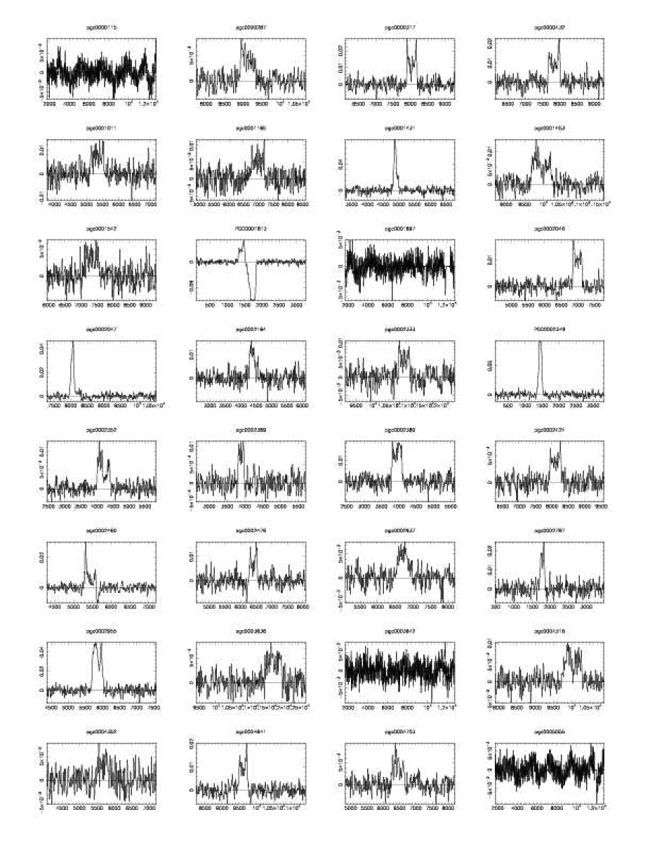
Figure 4: -excerpt. 21-cm line profiles of galaxies listed in Table 2; profiles are classified according to their PGC name which is written above each panel. Ordinate and abscissae axes are graduated respectively in km s^-1 and Jy. Note that heliocentric radial velocities are expressed in terms of optical redshift $c\frac{\Delta\lambda}{\lambda}$. The horizontal line represents the baseline of the profile, i.e. the zero flux level, from which the maximum is estimated.

3 Building the Tully-Fisher sample

3.1 The input data

Rotational velocities

Rotational velocities, i.e. the $\log{V_{m}}$ parameter used in the Tully-Fisher relation, have been mainly gathered from the HYPERLEDA compilation (16 666 galaxies, Paturel et al. 2003a ) and were complemented by some of our own recent HI line measurements with the Nançay radiotelescope (586 late type galaxies, Theureau et al. the05 (2005)). A few other measurements from Haynes et al. (hay99 (1999)) not previously in HYPERLEDA were also added. All our own 3300 HI spectra acquired with the Nançay radiotelescope antenna in the last decade were reviewed and assigned a quality code according to the shape of their 21-cm line profile. This study (Guilliard et al. gui04 (2004)) allows to flag efficiently several TF outliers due to morphological type mismatch or HI-confusion in the ellongated beam of Nançay. Even if this Nançay subsample concerns only a part of the data ($\sim$ 25%), we substantially improved the apparent scatter of the TF relation.

In the HYPERLEDA compilation, the $\log{V_{m}}$ parameter is calculated from 21-cm line widths at different levels and/or rotation curves (generally in H_α). The last compilation provides us with 50520 measurements of 21-cm line widths or maximum rotation velocity. These data are characterized by some secondary parameters: telescope, velocity resolution, level of the 21-cm line width. For data homogenization, HYPERELEDA uses the so-called EPIDEMIC METHOD (Paturel, G. et al. 2003b ). One starts from a standard sample (a set of measurements giving a large and homogeneous sample : here, the Mathewson et al. mat96 (1996) data), all other measurements are grouped into homogeneous classes (for instance, the class of measurements made at a given level and obtained with a given resolution). The most populated class is cross-identified with the standard sample in order to establish the equation of conversion to the standard system. Then, the whole class is incorporated into the standard sample. So, the standard sample is growing progressively. The conversion to the standard propagates like an epidemy. In summary, this kind of analysis consists in converting directly the widths for a given resolution r and given level l into a quantity which is homogeneous to twice the maximum rotation velocity ($=\log{W}$, uncorrected for inclination. A final correction is applied reference by reference to improve the homogenization.

The final $\log{V_{m}}$ value is corrected for inclination : $logV_{m}=(\log{W}-\log{(2\sin{incl})}$. Where the inclination $incl$ is derived following RC3 (de Vaucouleurs dev91 (1991)):

$$sin^{2}(incl)=\frac{1-10^{2logR_{25}}}{1-10^{2logr_{0}}}$$

$R_{25}$ is the axis ratio in $B$ at the isophot corresponding to 25 magȧrcsec^-2, $\log{r_{0}}$= 0.43 + 0.053$T$ for type $T$= 1 to 7 ($Sa$–$Sd$) and $logr_{0}$=0.38 for $T$=8 ($Sdm$).

Magnitudes

The 2MASS survey, carried out in the three infrared bands J, H and K, collected photometric data for 1.65 million galaxies with $K_{s}<14$ (Jarrett et al. jar00 (2000)) and made the final extended source catalog recently public. Total magnitude uncertainties for the 2MASS extended objects are generally better than 0.15 mag. We exclude any galaxy with the accuracy of magnitudes worse than 0.3. This accuracy appears reasonable when considering that it is almost impossible to obtain total magnitudes better than 0.1, due to the difficulty to extrapolate the profile in a reliable way.

Extinction

The extinction correction we applied includes a Galactic component, $a_{\rm G}$, adopted from Schlegel et al. (sch98 (1998)), and a part due to the internal absorption of the observed galaxy, $a_{\rm i}$. Both depend on the wavelength.

$$a_{\rm ext}=f_{\rm G}(\lambda)a_{\rm G}+f_{\rm i}(\lambda)a_{\rm i}.$$ (1)

The Galactic and internal wavelength conversion factors are $f_{\rm G}(\lambda)=$1.0, 0.45, 0.21, 0.13, 0.085 (Schlegel et al. sch98 (1998)) and $f_{\rm i}(\lambda)=$ 1.0, 0.59, 0.47, 0.30, 0.15 (Tully et al. tul98 (1998), Watanabe et al. wat01 (2001), Masters et al. mas03 (2003)) for B, I, J, H, and K bands, respectively.

Radial velocities

All radial velocities were taken from HYPERLEDA, often a mix and an average of several publications and redshift surveys. Within the limit of 8 000 km s^-1, we collected a sample of 32 545 galaxies. In general, when an HI measurement was available (i.e. for most of the TF subsample used in this study), the radio radial velocity was prefered, being more acurate than the available optical one. As it is the use in HYPERLEDA, when more than two redshift measurements for the same galaxy were available, the most discrepant ones were rejected from the mean. The radial velocities are used at the first iteration of the IND method as a reference distance scale for the Malmquist bias correction.

3.2 Selection and completeness

The analytical treatment of the Malmquist bias effect with distance, by applying the Iterative Normalized Distance method (IND), requires the strict completeness of the samples according to magnitude selection (Theureau et al. 1998b and Sect. 4.). The limits in magnitude are simply determined by eye as the knee observed in a $\log{N}$ vs. magnitude diagram, witnessing the departure from a homogeneous distribution in space with growing distance. This limit is in ’observed apparent magnitude’, independently of extinction or opacity correction. These corrections however are taken into account further, as part of the ND scheme itself, in what we call the effective magnitude limit (Sect. 4.1.).

The adopted completeness limit are the followings : J_lim=12.0, H_lim=11.5, and K_lim=11.0 (equivalent to B${}_{\rm lim}\sim$ 15 and I${}_{\rm lim}\sim$ 13). Only the complete part of the sample in each band, about half of available data, is included for further study.

The final selection is made according to the following conditions:

• J, H, and K magnitudes $<$ completeness limit

• magnitude uncertainty $<$ 0.3 mag

• log of rotational velocity uncertainty $<$ 0.03

• $T$ = 1–8 to keep only fair spiral galaxies

• $\log R_{25}>0.07$ to avoid face-on galaxies for which the rotational velocity is poorly determined

After these restrictions there are 3263 spiral galaxies distributed over the whole sky (see Fig. 5).

Figure 5: Sky distribution of KLUN galaxies used in the current analysis

4 Method of analysis

In this section we explain the Iterative Normalized Distance method for deriving the peculiar velocities. The ’iterative’ means that a previously calculated peculiar velocity field is used for a more accurate estimation of new peculiar velocities. The ’normalized distance’ is a quantity depending on the distance and the absolute size or absolute magnitude of a galaxy, such that for any galaxy, the average selection bias (in the terminology of Strauss & Willick, str95 (1995)) or the Malmquist bias of the second kind (according to Teerikorpi, tee97 (1984)) can be given by a function depending on its normalized distance, the dispersion of the distance criterion, and the completeness limit. This is illustrated in Fig. 6, where the TF residuals, plotted against the normalized distance modulus, clearly show the unbiased regime and the deviation due to the magnitude cutoff.

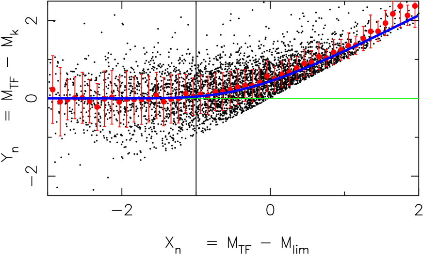
Figure 6: TF residuals ($Y_{\rm n}$ against the normalized distance modulus ($X_{\rm n}$). The “unbiased plateau” is the region at $X_{\rm n}<-1$, where the binned average of the residuals, the balls with error bars, are close to the zero line. The curve going through the balls is the analytical correction formula described by Eq. 8 in Sect. 4.1.

A fully detailed description of the method follows, but we start by listing the main steps:

1. Calculate the absolute magnitudes and the normalized distances using the kinematical (redshift) distances.

2. Calculate the TF relation using the unbiased part of the normalized distance diagram.

3. Use the unbiased TF relations and the analytical Malmquist correction formula for estimating real space galaxy distances beyond the unbiased plateau limit (Fig5̇).

4. Obtain the peculiar velocity field in a Cartesian grid in the redshift space by smoothing the individual peculiar velocities given by the Malmquist corrected TF distances.

5. Go back to step 1, and use the corrected kinematical distances by substracting the smoothed peculiar velocity field values from the redshift velocities.

This loop is repeated until converging values for the peculiar velocities are obtained. The peculiar velocities for all the galaxies do not converge nicely, though. We thus extract the most unreliable galaxies (about 4 %) and recalculate the velocities with the reduced data set (see Sect. 4.4. and Fig. 6). As confirmed by the tests done with a mock sample in Sect. 4.6. outliers use to be mainly very low Galactitic latitude objects for which the corrected total magnitude is not well estimated from observed one, and core cluster members whose observed radial velocity, used as kinematical distance at the first iteration, does not reflect at all their true distance, due to their strong motion in the cluster potential.

4.1 Kinematical distances, normalized distances and absolute magnitudes

Let us define the kinematical distance modulus as

$$\mu_{\rm k}=5\log\frac{cz}{H_{0}}+25,$$ (2)

where $cz$ is the observed heliocentric redshift, corrected by the CMB dipole motion. The absolute magnitude is

$$M_{\rm k}=m_{0}^{\rm c}-\mu_{\rm k}$$ (3)

where $m_{0}^{\rm c}$ is the apparent magnitude, corrected for inclination, extinction, and cosmological effects, as stated in Eq. 10 of Paturel et al. (pat97 (1997)) (the cosmological correction is negligible for all galaxies in the present study).

If we consider that the TF relation is a linear law characterized by a given slope and a given dispersion (the zero-point being fixed either by some local calibrators or by adopting a value of $H_{0}$), and if we assume that the sample is actually complete up to a well defined apparent magnitude limit, then the selection bias at a fixed $\log{V_{\rm m}}$ is only a function of the distance (see Teerikorpi tee84 (1984), Theureau et al. the97 (1997), 1998b ). In other words, the bias at a fixed $\log{V_{\rm m}}$ and at a given distance is only the consequence of the magnitude cut-off in the distribution of TF residuals and moreover it does not depend at all on space density law.

By normalizing to a same luminosity class, i.e. a same $\log{V_{\rm m}}$ value, and by taking into account the variation of the actual magnitude cut-off with extinction, one can build a unique diagram showing the bias evolution with distance.

The distances and magnitudes are then scaled so that a sharp edge is seen at the sample completeness limit.

The normalized distance modulus is defined as

$$X_{\rm n}=\mu_{\rm k}+(M_{\rm TF}-m_{\rm lim}+a_{\rm ext})$$ (4)

where $M_{\rm TF}$ is the absolute magnitude of a galaxy, as given by the Tully-Fisher relation and $m_{\rm lim}$ is the apparent magnitude completeness limit. More explicitely, if we develop $M_{\rm TF}$ as $[a_{1}\log{V_{\rm m}}+a_{0}]$ it appears that we normalize indeed to the same $\log{V_{\rm m}}$ and the same effective magnitude limit $m_{\rm lim}^{\rm eff}=m_{\rm lim}-a_{\rm ext}$. $X_{n}$ can also be expressed as $M_{\rm TF}-M_{\rm lim}$, i.e. the difference between the TF absolute magnitude at a given $\log{V_{\rm m}}$ and the absolute magnitude cut off (in the TF residuals) at a given distance.

The normalized magnitude

$$Y_{\rm n}=M_{\rm TF}-M_{\rm k}=M_{\rm TF}-m_{0}^{\rm c}+\mu_{\rm k}$$ (5)

corresponds to the departure of the absolute magnitudes calculated on the basis of kinematical distances from the true mean value given by the TF relation. This residual contains the contribution of magnitude and $\log{V_{\rm m}}$ measurement errors, internal TF dispersion, and peculiar velocity.

Figure 6 shows normalized distance moduli vs. normalized magnitudes for the galaxies derived by the Tully-Fisher relation. The curve going through the points is the analytical bias solution $f(X_{\rm n},\sigma_{\rm TF},m_{\rm lim})$ while the vertical line shows the upper limit adopted for the unbiased normalized distance domain.

4.2 Unbiased Tully-Fisher

The TF relation states the linear connection between absolute magnitude and $\log V_{\rm m}$

$$M=a_{1}\log V_{\rm m}+a_{0}$$ (6)

One gets the slopes, $a_{1}$, and zero-points, $a_{0}$, of the TF relations in each band ($IJHK$) by least squares fit using the unbiased part of each sample. The unbiased part is the flat or plateau region in the normalized distance diagram. This subsample also provides us with the ”0-value” of the TF residuals that is used to compute the bias deviation for the whole magnitude complete sample (the horizontal line in Fig. 6). The method of deriving the TF relation in the unbiased plateau has been succesfully used in previous KLUN studies; a full statistical description can be found in Theureau et al. 1998b and it was even numerically tested by Ekholm (ekh97 (1997)).

In the iterative scheme one starts by assuming a priori values for the TF slope and zero-point (here, only the slope is important and a rough value can be inferred directly from the whole sample). These values are used to compute the normalized distance and extract a first unbiased subsample. The loop ”TF-slope $\rightarrow$ normalized-distance $\rightarrow$ unbiased-subsample $\rightarrow$ TF-slope” can be repated a couple of times to be sure to start on the basis of unbiased values.

4.3 Corrected distances

The function $f(X_{\rm n},\sigma_{TF},m_{\rm lim})$ is deduced from the expectancy of $Y_{\rm n}$ knowing $X_{\rm n}$ assuming that the magnitude selection $S(m)$ is described by the Heavyside function $S(m)=\theta(m-m_{\rm lim})$. We have then:

$$E(Y_{\rm n}|X_{\rm n})=\frac{1}{B}\int_{Y_{\rm lim}}^{-\infty}\frac{1}{\sqrt{2\pi}\sigma}Y\exp[-\frac{Y^{2}}{2\sigma^{2}}]dY$$ (7)

where

$$\sigma=\sigma_{\rm TF}$$

$$Y_{\rm lim} = Y_{\rm n}(m_{\rm lim})=M_{\rm TF}-m_{\rm lim}^{\rm eff}+\mu_{\rm k}$$

$$= M_{\rm TF}-(m_{\rm lim}-a_{\rm ext})+\mu_{\rm k}$$

$$\equiv X_{\rm n}$$

$$B=\int_{Y_{\rm lim}}^{-\infty}\frac{1}{\sqrt{2\pi}\sigma}\exp[-\frac{Y^{2}}{2\sigma^{2}}]dY$$

From here we derive:

$$f(X_{\rm n},\sigma,m_{\rm lim})=\sigma\,\sqrt{\frac{2}{\pi}}\,\frac{e^{-A^{2}}}{{\rm erfc}(A)}$$ (8)

where,

$$A=-\frac{1}{\sqrt{2}\sigma}X_{\rm n}$$

and

$${\rm erfc}(x)=\frac{2}{\sqrt{\pi}}\int_{x}^{-\infty}{e^{-y^{2}}dy}$$

The corrected and unbiased distance modulus is then finally:

$$\mu_{c}=m^{c}-M_{\rm TF}+f(X_{\rm n},\sigma,m_{\rm lim})$$

Note that $H_{0}$ is cancelled out in $Y_{lim}$: it is indeed hidden in the TF zero-point and explicitely present in $\mu_{k}$ but with an opposite sign.

The reader will remark that our approach to the bias in this paper is radically different to what has been attempted with MarkIII (Willick et al wil97 (1997) or Dekel et al dek99 (1999)) in which the approach has been from the viewpoint of the classical Malmquist bias (using in particular some inhomogeneous density correction).

4.4 Iterations

The peculiar velocities of galaxies are then smoothed onto a cartesian grid, $v_{\rm pec}(x,y,z)$ (Sect. 4.5). As explained above, the method relies on kinematical distances; the normalized distances and the absolute magnitudes needed for TF relation include the kinematical distance. These distances can be made more accurate by subtracting the peculiar velocities from the redshift:

$$\mu_{\rm k}=5\log\frac{cz-v_{\rm pec}(x,y,z)}{H_{0}}+25.$$ (9)

This distance modulus then replaces the value given by Eq. 2, and we can repeat the whole procedure with these updated distances. The new peculiar velocity field is again used for correcting the kinematical distances in the next iteration, and we keep on repeating the process until convergence.

In practise, subtracting the whole $v_{\rm pec}(x,y,z)$ as in Eq. 9 would overcorrect for the peculiar velocities, and cause diverging oscillatory behaviour in the iterative process. Using a scaling factor $\lambda\in(0.0,1.0)$ so that

$$\mu_{\rm k}^{j+1}=5\log\frac{cz-\lambda\,v_{\rm pec}^{j}(x,y,z)}{H_{0}}+25,$$ (10)

removes this problem. The superscript $j$ corresponds to the iteration number. Using the value $\lambda=0.5$ we reach converging values after about 5–10 iterations. Figure 7 shows this convergence for a few galaxies. Usually the $v_{\rm pec}^{j}$ approaches nicely to a constant value, in some cases the values oscillate even with high $j$. We checked all these convergence curves by eye and rejected the worst cases. With the restricted sample we recalculated the peculiar velocities and used the results of the selected 3126 spirals galaxies for the peculiar velocity mapping.

Figure 7: The evolution of peculiar velocities with respect to the number of iterative loop. Here are the two first galaxies in our sample, and an exceptionally “bad” case (pgc 17978) which was rejected from the final analysis.

4.5 The tensor smoothing

After deriving radial peculiar velocities of galaxies it is useful to interpolate these velocities at uniformly distributed grid points. The best method is to smooth the observed galaxy velocities with an appropriate window function. Dekel et al. (dek99 (1999)) discuss the problems of smoothing a non-uniformly distributed set of radial velocities:

The radial velocity vectors are not all pointing in the same direction over the smoothing window. Then, for example in a case of a pure spherical infall towards the window center, all the transverse velocities are observed as negative radial velocities. The net velocity in the smoothing window is then, incorrectly, negative, in stead of being zero. Dekel et al. (dek99 (1999)) call this the tensor window bias. They find that it can be reduced by introducing a local velocity field with extra parameters, which is to be fitted for the observed radial velocities in the smoothing window. The best results are obtained by constructing a three-dimensional velocity field with a shear,

$${\bf v}({\bf x})={\bf B}+{\bf L}\cdot({\bf x}-{\bf x}_{\rm c}),$$ (11)

where ${\bf L}$ is a symmetric tensor, and ${\bf x}_{\rm c}$ is the window center. There are then nine free parameters, three for the actual window center velocity ${\bf B}$ and the six components of the tensor ${\bf L}$. The resulting grid point velocity is just ${\bf v}({\bf x}_{\rm c})={\bf B}$.

Furthermore, if the true velocity field has gradients within the effective smoothing window, a nonuniform sampling will cause an error, called the sampling-gradient bias. Dekel et al. (dek99 (1999)) suggest that this bias can be diminished by weighting the observed galaxy velocities by the volume $V_{n}$, which is defined as the cube of the distance between the galaxy and its $n$th neighbour. This method gives more weight for galaxies in isolated areas.

4.6 Testing the method

We test these biases with a mock peculiar velocity catalog. The mock catalog is constructed from the GIF consortium constrained n-body simulation of our $80h^{-1}$ Mpc neighbourhood (Mathis et al. mat02 (2002), http://www.mpa-garching.mpg.de/NumCos/CR/). The simulation was run for a flat $\Lambda$CDM cosmological model, and it provides locations, velocities, masses, and luminosities, with and without the internal absorption, of 189 122 galaxies. The galaxy formation was defined by applying a semianalytic algorithm on the dark matter merger tree. We added the Galactic component of the absorption, as defined in Schlegel et al. (sch98 (1998)), and selected the galaxies brighter than a magnitude limit. In the end there are 9800 galaxies with their apparent B band magnitude smaller than 14.5.

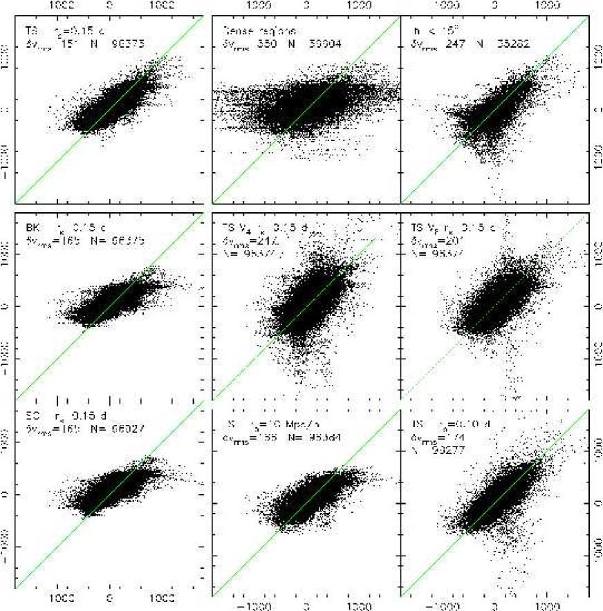
Figure 8: Shown here are the true peculiar velocities (on y axis) vs. the velocities obtained with a smoothing method for the GIF consortium simulated data. The upper left corner of each panel gives the essential information about the plot; TS stands for the tensorial smoothing, using nine parameters, the bulk velocity B and the tensor L, BK is the three parameter bulk smoothing (only B), and SC means scalar smoothing, using a simple Gaussian smoothing window. $r_{s}$ is the smoothing radius, either a distance dependent value, e.g. $0.15d$ or a fixed value, e.g. 10 Mpc $h^{-1}$. The rms difference between the smoothed and the true velocity field, $\delta v_{\rm rms}$, is given in km s^-1. N is the number of points, the simulated galaxies, in each figure. Upper left figure shows the smoothing giving the smallest $\delta v_{\rm rms}$. In each figure the galaxies in densest regions were excluded, as well as the objects at the low Galactic latitudes. The two panels in the upper right corner show how these points give substantially more divergent values. The “Dense regions” and “$|b|<15^{o}$” maps were obtained with the TS $r_{s}=0.15d$ smoothing. V₄ and V₈ correspond to the volume weighted method, using the volume defined by the fourth and the eight closest galaxy, respectively. The volume weighting is claimed to reduce the sampling gradient bias, but in this test they fail to produce a better estimate of the true velocity field than the non-weighted method.

Figure 8 shows the true vs. smoothed peculiar velocities using different smoothing method and set of window parameters. These plots lead to the following comments:

• the scatter is mainly related to the smoothing radius

• outliers are essentially:
  - galaxies at low Galactic latitude, for which the magnitude is not well defined and where the sparser sampling leads the smoothing to diverge (vertical spreading)
  - galaxies belonging to clusters for which the kinematical distance derived from the redshift is strongly affected by the cluster velocity dispersion

• one observes a tilt with respect to the line with slope = 1, when no tensor window is used. This is the effect of the velocity gradient around structures and leads to an underestimation of infall patterns and to a cooler velocity field.

The best $\chi^{2}$ value is obtained for $\rm B+L$ smoothing, and $R_{smooth}=0.15\times distance$. This will be our choice of smoothing for the rest of the study.

5 Preliminary results

In this section we present the TF relation parameters obtained for three wavelengths (JHK) and some examples of maps of radial peculiar velocity fields, superimposed on the distribution of galaxies. A more detailed kinematical study is beyond the scope of the present analysis and will be presented in a forthcoming paper.

5.1 TF parameters

Figures 9 show the final TF relations for the galaxies in the unbiased part of the normalized distance diagram. Tables 4– list the parameters $a_{1}$ and $a_{0}$ and the scatter of the relation :

$$M=a_{1}\log V_{\rm m}+a_{0}$$ (12)

Figure 9: Tully-Fisher relations in J, H, and K bands for unbiased plateau galaxies. See Table 4 for the parameters of the relations.

Table 4: Tully-Fisher parameters: slope, zeropoint, scatter, and the number of unbiased plateau galaxies used in the relation.

	$a_{1}$	$a_{0}$	$\sigma_{\mathrm{T}F}$	$N$
J	-6.3 $\pm$ 0.31	-8.8 $\pm$ 0.14	0.46	960
H	-6.4 $\pm$ 0.33	-9.1 $\pm$ 0.14	0.47	1166
K	-6.6 $\pm$ 0.37	-9.0 $\pm$ 0.16	0.45	990

The observed scatter is comparable to what was found by Karachentsev et al kar02 (2002) using 2MASS magnitudes. The small difference (we get slightly smaller $\sigma$’s) can be explained easily by our optimization of the kinenatical distance scale through the iterative process described above. Accounting for the observed broadening due to apparent magnitude and $\log{V_{max}}$ uncertainties and to the residual peculiar velocity dispersion affecting the kinematical distances, one obtains an internal scatter of $\sim$ 0.44 mag for the TF relation in $B$ and $\sim$ 0.4 mag in $K$. This is 0.1 mag greater than in studies restricted to pure rotation curve measurements of $\log{V_{max}}$. Here instead, a large majority of $\log{V_{max}}$ measurement are from the width of global HI profiles. As we know, even once corrected for non-circular motions, this width is still determined by the shape of a galaxy’s rotation curve, the distribution of HI gas in the disk and the possible presence of a warp (Verheijen ver01 (2001)), leading to a greater intrinsic Tully-Fisher scatter.

5.2 Peculiar velocities

Table 5 shows the first 10 KLUN+ galaxies with TF distances. The distances are expressed in km s^-1. That is followed by the kinematical distance, corrected by the radial peculiar velocity. This is our estimate of the true distance of a galaxy. Finally we list the observed redshift velocity in the CMB rest frame. The full catalog is given in electronic format only.

Table 5: An excerpt of the table showing the distance data. We list the name and the galactic coordinates of the galaxies, followed by the three TF distances. Then we give the corrected kinematical distance, $d_{\rm k}^{\rm c}=V_{\rm 3k}-V_{\rm pec}$. All are expressed in km s^-1. The last entry is the redshift velocity, corrected to the CMB rest frame.

	$l$	$b$	$d_{\rm TF,J}$	$d_{\rm TF,H}$	$d_{\rm TF,K}$	$d_{\rm k}^{\rm c}$	$V_{\rm 3k}$
PGC 2	113.96	-14.70	6084	6030	5992	4762	4751
PGC 54	109.57	-33.17	8864	8936	9152	8771	8379
PGC 76	109.81	-32.67	7997	7592	—	6968	6570
PGC 102	111.34	-27.22	5214	5125	5211	4834	4720
PGC 112	110.61	-30.23	4961	4754	4764	4493	4449
PGC 120	108.40	-37.98	3893	3771	3815	4202	4051
PGC 129	108.42	-37.97	6413	6155	6105	4177	4026
PGC 176	94.33	-63.84	7662	7359	—	6412	6117
PGC 186	107.24	-42.50	9047	8557	9158	8034	7541
PGC 195	355.68	-77.39	6281	5862	6319	6254	6538

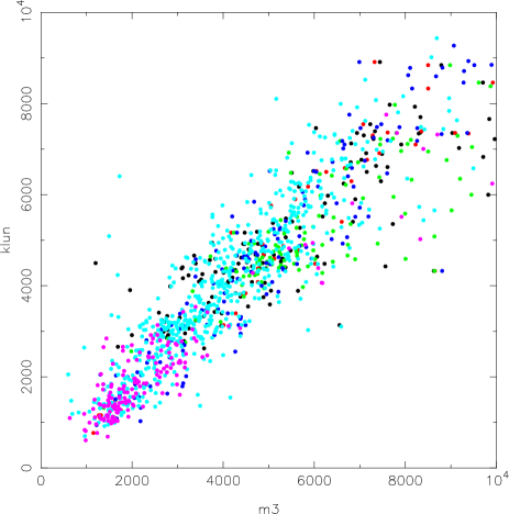
Figure 10: Comparison of MarkIII and KLUN distances expressed in km.s^-1. The colors represent the different Mark III samples (Willick et al. wil97 (1997)): HMCL is black, W91CL red, W91PP green, CF blue, MAT turquoise, and A82 purple.

Our peculiar velocities were obtained for all points in space having large enough galaxy density. We required that there should be more than 15 galaxies with peculiar velocity measurements within the smoothing radius around the point. Then we fit the 9-parameter tensor field to the peculiar velocities of these galaxies and set the value obtained at the center of the smoothing window (see Sect. 4 for more details).

Since we use a distance dependent smoothing radius, the points close the Local Group must have a higher density of KLUN galaxies around them than the more distant points, for a succesful velocity field determination. This explains why some of the more distant grid points have a set value while there are apparently no galaxies around them.

We compared the data to the MarkIII distances (Willick et al. wil97 (1997)). Mark III catalog was compiled from six samples of TF and one of elliptical galaxies. It was converted to a common system by adjusting the zero points of the distance indicators. For the Malmquist bias correction the authors reconstructed the galaxy density field from the IRAS 1.2 Jy survey, and used it for the inhomogeneous correction formula. The corrected distances for 2898 spirals and 544 ellipticals are publically available and make a good comparison point for other peculiar velocity studies.

Figure 10 show the Malmquist corrected distances of individual galaxies, as measured in Mark III, versus the corresponding value derived by us. The relative scatter $\sigma_{d}/d$ is $\sim$ 0.2, correponding to an absolute uncertainty 0.43 in magnitude scale, is fully compatible with the measured TF scatter (see Table 4). A few points in Figure 10 show a clear mismatch. We found that these large discrepancies are due to errors in the input data in Mark III. These errors are listed and discussed in Appendix A.

Figure 11 shows the radial peculiar velocity field in the supergalactic plane, averaged over a disc having a thickness that increases towards the edge. The thickness of the disc in the center is zero, and its opening angle is $15\degr$, so that at the edge (at 80 h^-1 Mpc) the disk width is about 20 h^-1 Mpc. The blue colors refer to regions where the radial peculiar velocity is towards us, the red regions are outfalling. The shade of the color corresponds to the amplitude of the motion, and is saturated at 1 000 km s^-1. The regions where the threshold requirement of at least two velocity measurements is not satisfied are set white. The black dots are galaxies in HYPERLEDA with measured redshifts (not just the KLUN galaxies). Green circles mark some well known clusters. The maps are in real space coordinates, i.e. the redshift distances corrected by the peculiar velocity field.

It is worth noting that in our $v_{\rm pec}$ maps one observes both the front and backside infall patterns around the main superclusters and structures. It is particularly obvious on Fig. 11 for the regions of Virgo, Perseus-Pisces, N533, Norma, or even Coma, though it is located close to the limit of the sample. It seems that we even detect an outflow in the front side of the Great Wall. Similar features are seen on Fig. 12 that shows other slices with different orientations in space.

A wide region however, roughly centered on Centaurus cluster, seems to move away from us at a coherent speed of $\sim$400 km s^-1 on a scale greater than $20h^{-1}$ Mpc. The direction and amplitude of this bulk motion are close to the one of the putative Great Attractor (Lynden-Bell et al lyn88 (1988), Hudson et al hud04 (2004), Radburn-Smith rad06 (2006)) and cannot be associated to any structure in particular. Anyway, it seems that this flow vanishes beyond a distance of $50h^{-1}$ Mpc.

Figure 11: Radial peculiar velocity field in the supergalactic plane. Blue colors are regions with negative peculiar velocities, red colors refer to positive ones. Black dots are all galaxies with a known redshift. Green marks show positions of some well known structures – here Virgo, Ursa Major, Norma, Pisces, N533, and Zwicky33. The coordinates are in “real space”, i.e. redshift distances corrected for the smoothed peculiar velocity field, in units of km s^-1.

Figure 12: The peculiar velocity maps, as in Fig. 11, projected on four discs of different orientations with respect to the supergalactic plane (SGZ=0). Figure a is rotated by 10°around the SGX axis. It illustrates well the features around two large rosary structures: the Great Wall starting from Coma and extending counterclockwise up to the Centaurus region, and another starting from Perseus-Pisces complex, going down through N533 and beyond. Both front and backside infall are visible all along the structures. Figure b is rotated by -30°around SGZ from the SGY=0 plane, and shows the large infall motions towards the two opposite regions, one in Perseus-Pisces and the other in the Great Attractor or Centaurus area. Figure c, rotated 50°around SGY from the SGX=0 plane, shows the infall patterns towards Pegasus, Hydra, and Coma. Figure d, that is almost perpendicular to the supergalactic plane, rotated -30°around SGY from the SGX=0 plane, shows an example of some very detailed structure of the velocity field.

Figure 13: Upper panel shows the amplitude of the observed bulk motion within a growing sphere of radius $R_{\rm max}$, and the corresponding $\Lambda$CDM expected curve for a flat cosmological model using : $n=1$, $\Omega_{b}=0.04$, $h=0.57$, and $\Omega_{m}$ = 0.22 $\pm$ 0.02 . The bottom panel show the direction of the bulk flow, in galactic coordinates, and its evolution with $R_{\rm max}=10$–$60h^{-1}$ Mpc. The main published results as listed in Table 6 are also shown.

As an example of quantitative result, we checked the amplitude and direction of a bulk flow within a growing sphere centered on the Local Group. The result is shown on Fig. 13.

At short scales the direction of the flow is compatible with most previous studies (Table 6, Fig. 13, bottom panel). In particular it coincides with the Great Attractor for $R\sim 20h^{-1}$ Mpc. At larger scales it first drifts towards the direction of the rich cluster region of Horologium–Reticulum, and after $R\sim 40h^{-1}$ Mpc back to $(l,b)\sim(310\degr,-8\degr)$.

In the upper panel, we show the bulk flow amplitude within a sphere of growing radius (colored line). It oscillates strongly at short scales, as a consequence of the density heterogeneity, and decreases to $\sim 250$ km s^-1 at 40 h^-1 Mpc. Beyond this point it behaves more smoothly, as an indication that we reached the scale of the largest structures within our sample. It starts to rise (or oscillate) again beyond 60 h^-1 Mpc, probably due to the sparser space sampling.

The black solid curve shows the rms expected bulk velocity infered from the standard $\Lambda$CDM model:

$$V_{b}^{rms}=\langle v^{2}(R)\rangle^{1/2}=\left(\frac{\Omega_{m}^{1.2}}{2\pi^{2}}\int_{0}^{\infty}P(k)\tilde{W}^{2}(kR)dk\right)^{1/2},$$

where $P(k)$ is the mass fluctuation power spectrum and $\tilde{W}^{2}(kR)$ is the Fourier transform of a top hat window of radius $R$. For the parametric form of $P(k)$ in the linear regime, we use the general CDM model (see e.g. Silberman et al., sil01 (2001)) :

$$P(k)=A_{c}(\Omega_{m},\Omega_{\Lambda},n)T^{2}(\Omega_{m},\Omega_{b},h;k)k^{n}$$

$A_{c}$ is the normalization factor and the transfer function $T(k)$ is the one proposed by Sugiyama (sug95 (1995)). We restricted the analysis to a flat cosmological model with $\Omega_{m}+\Omega_{\Lambda}=1$, a scale-invariant power spectrum ($n=1$), a baryonic density $\Omega_{b}=0.04$ (WMAP result, e.g. Spergel spe06 (2006)), a Hubble constant fixed at $h=0.57$ (which is our own preferred value, inferred directly from primary calibration by Theureau et al the97 (1997)), adjusting only the value of $\Omega_{m}$.

The best fit has been obtained for $\Omega_{m}=0.22$ in the distance range 40-60 Mpc, where the value of $\langle V_{rms}(R)\rangle$ appears very smoothed. We also ploted the $\pm$ 0.02 curves around this best value. What we observe confirms WMAP results on $\Omega_{m}$ (e.g. Spergel spe06 (2006)) and seems coherent with the expected rms bulk velocity within a sphere for standard $\Lambda$CDM model (see e.g. Willick wil00 (2000) or Zaroubi zar02 (2002)), thus with no bulk motion.

One should be prudent anyway in such kind of conclusion : the theoretical prediction is here the rms value of a quantity that exhibits a Maxwell distribution (see e.g. Strauss str97 (1997)); a single measurement of the flow field is only one realization out of this distribution and gives only very weak constraints on the cosmological model.

Table 6: Directions, in Galactic coordinates, of some of the main bulk flow measurements or large galaxy concentrations. The number corresponding to Fig. 13 is given in parentheses.

	$l$	$b$	ref.
SNIa (1)	282	-8	Riess et al. rie97 (1997)
ENEAR (2)	304	25	da Costa et al. 2000a
SFI+SCI+II (3)	295	25	Dale & Giovanelli dal00 (2000)
SMAC (4)	260	-1	Hudson et al. hud99 (1999)
PSCz (5)	260	30	Rowan-Robinson et al. row00 (2000)
LP	343	52	Lauer & Postman lau94 (1994)
CMB	276	30	Local Group motion, Kogut et al. kog93 (1993)
GA	307	9	Great Attractor, Lynden-Bell et al. lyn88 (1988)
HR	270	-55	Horologium–Reticulum, Lucey et al. luc83 (1983)
SC	315	29	Shapley Concentration, Scaramella et al. sca89 (1989)

Appendix A Mark III errata & rejections

When closely inspecting the Mark III data we found a few inaccuracies. In comparison we used the Mark III catalog provided by the CDS archives, http://cdsweb.u-strasbg.fr, cat. VII/198, and the data given by the HYPERLEDA database, http://leda.univ-lyon1.fr, as they were presented in May 2003. A few values in Mark III were replaced by those listed in HYPERLEDA. Some of the Mark III galaxies were rejected, having large differences to the HYPERLEDA values.

Table 7 lists galaxies having their PGC numbers incorrectly identified in Mark III. We list first the number given in Mark III, followed by the correct number, alternative name, and the Mark III data set including the galaxy.

Table 7: Mark III errata: PGC numbers.

Mark III	correct	alt. name	Mark III data sets
PGC 106311	PGC 95735	—	HMCL, W91CL, CF
PGC 64575	PGC 64632	NGC 6902	HMCL
PGC 57053	PGC 57058	UGC 10186	W91CL
PGC 71291	PGC 71292	UGC 12572	W91CL

1) PGC 10631 = UGC 2285 is projected on PGC 95735, but at lower redshift. Mark III clearly refers to the latter, but lists it as UGC 2285.

Table 8 lists galaxies that were rejected due to their suspicious values for redshift velocities (values given in the CMB rest frame). All the galaxies with $|cz_{\mathrm{M}3}-cz_{\mathrm{H}L}|>200$ km s^-1 were studied, for most we maintained the Mark III values.

Table 8: Mark III errata: velocities.

	Mark III	HYPERLEDA	Mark III data sets
PGC 26680	7266	12736	HMCL
PGC 72301	11747	7348	W91PP
PGC 171361	4417	8870	CF
PGC 265612	2136	1664	MAT
PGC 67258	2278	2684	MAT
PGC 62889	2513	5745	MAT
PGC 307533	2946	3813	MAT
PGC 9551	4057	4633	MAT
PGC 203244	4114	5681	MAT
PGC 15790	4202	6199	MAT
PGC 47832	4477	4827	MAT
PGC 317235	4866	4130	MAT
PGC 624116	5075	5996	MAT
PGC 5964	5859	5406	MAT
PGC 3144	5974	5053	MAT
PGC 8888	6070	5049	MAT
PGC 64523	6384	5271	MAT
PGC 19363	7092	6666	MAT
PGC 2001	7112	6180	MAT
PGC 44349	9696	9916	MAT

1) Value incorrectly copied from the data source
2) Lower value suggested by three independent sources
3) See note at Giovanelli et al. gio97 (1997) (Antlia 27146)
4) Possible confusion with galaxy 1’ SE
5) A typographical error in MAT file? See Mathewson et al. mat92 (1992), Fig. 3
6) Unclear H$\alpha$ observation

Table 9 has the galaxies rejected due to the $\log V_{\rm m}$ uncertainties. Here we considered galaxies with $|\log V_{\rm m,M3}-\log V_{\rm m,HL}|>0.15$. Notice that Mark III $\log W$ values are here converted to the inclination corrected $\log V_{\rm m}$ of HYPERLEDA.

Table 9: Mark III errata: $\log V_{\rm m}$.

	Mark III	HYPERLEDA	Mark III data sets
PGC 72024	2.321	2.131	HMCL,W91CL,W91PP,CF
PGC 477071,2	2.139	2.391	HMCL
PGC 653381	2.079	1.844	HMCL
PGC 71111	1.978	2.251	HMCL
PGC 368751	2.253	2.453	W91CL
PGC 98413	2.049	1.596	W91PP
PGC 51784	2.209	1.889	CF
PGC 5453	2.429	1.980	CF
PGC 171131	1.994	1.830	MAT
PGC 16201	1.807	2.092	MAT
PGC 328211	2.023	1.861	MAT
PGC 678181	2.052	1.843	MAT
PGC 39139	1.760	2.018	MAT
PGC 519821	2.284	2.057	MAT
PGC 24328	2.232	2.013	MAT
PGC 640421	2.442	2.200	MAT
PGC 137781	2.295	2.123	MAT
PGC 2383	1.978	2.150	MAT
PGC 368751	2.241	2.453	A82

1) These galaxies have large differences in inclination stated in Mark III and in HYPERLEDA.
2) Mark III states the inclination as $90\degr$, while it is $34\degr$ in HYPERLEDA. The latter is probably correct.
3) Several sources favour the HYPERLEDA value.

References

- (1) Barnes, D. G., Staveley-Smith, L., de Blok, W. J. G., et al 2001, MNRAS 322, 486
- (2) Bottinelli, L., Gouguenheim, L., Fouqué, P., Paturel, G., 1990, A&AS 82, 391
- (3) Bottinelli, L., Durand, N., Fouque, P., Garnier, R., Gouguenheim, L., Paturel, G., Teerikorpi, P., 1992, A&AS93,173
- (4) Bottinelli, L., Durand, N., Fouque, P., Garnier, R., Gouguenheim, L., Loulergue, M., Paturel, G., Petit, C., Teerikorpi, P., 1993, A&AS 102,57 (paper II)
- (5) da Costa, L.N., Bernardi, M., Alonso, M.V., et al. 2000a, ApJ, 537, L81
- (6) da Costa, L.N., Bernardi, M., Alonso, M.V., et al. 2000b, AJ, 120, 95
- (7) Dale, D.A. & Giovanelli, R. 2000, Cosmic Flows Workshop, ASP Conf. Ser., Vol. 201. Ed. by S. Courteau and J. Willick, p.25
- (8) Dekel, A., Eldar, A., Kolatt, T. et al. 1999, ApJ, 522, 1
- (9) Ekholm, T. 1996, A&A, 308, 7
- (10) Ekholm, T., Teerikorpi, P., Theureau, G. et al. 1999, A&A, 347, 99
- (11) Fouqué, P., Bottinelli, L., Gouguenheim, L., Paturel, G., 1990, ApJ349,1
- (12) Giovanelli, R., Haynes M.P., Herter T., et al. 1997, AJ, 113, 22
- (13) Guilliard, P., 2004, Master Thesis
- (14) Hanski, M.O., Theureau, G., Ekholm, T., Teerikorpi, P. (2001, A&A378, 345)
- (15) Haynes M.P., Giovanelli R., Chamaraux P., et al. 1999, AJ, 117, 2039
- (16) Hudson, M.J., Smith, R.J., Lucey, J.R., Schlegel, D.J. & Davies, R.L. 1999, ApJ, 512, L79
- (17) Hudson, M.J.; Smith, R.J.; Lucey, J.R.; Branchini, E. 2004, MNRAS352, 61
- (18) Jarrett, T.-H., Chester, T., Cutri, R. et al. 2000, AJ, 120, 298
- (19) Karachentsev I.D., Mitronova S.N., Karachentseva, V.E., Kudrya, Yu.N., & Jarrett, T.H. 2002, A&A, 396, 431
- (20) Kogut, A., Lineweaver, C., Smoot, G.F. et al. 1993, ApJ, 419, 1
- (21) Lauer, T.R. & Postman, M. 1994, ApJ, 425, 418
- (22) Lucey, J.R., Dickens, R.J., Mitchell, R.J. & Dawe, J.A. 1983, MNRAS, 203, 545
- (23) Lynden-Bell, D., Faber, S.M., Burstein, D. et al. 1988, ApJ, 326, 19
- (24) Mamon, G., Giraud, F., Rassia, E. et al. 2004, in Maps of the Cosmos, International Astronomical Union. Symposium no. 216, held 14-17 July, 2003 in Sydney, Australia
- (25) Marinoni, C., Monaco, P., Giuricin, G., Costantini, B. , 1998, ApJ505, 484
- (26) Masters, K., Giovanelli, R., Haynes, M., 2003, AJ126, 158
- (27) Mathewson, D.S., Ford, V.L. & Buchhorn, M. 1992, ApJS, 81, 413
- (28) Mathewson, D.S. & Ford, V.L. 1996, AJ, 107, 97
- (29) Mathis, H., White, S. 2002, MNRAS, 337, 1193
- (30) Mitronova, S.N., Karachentsev, I.D., Karachentseva, et al ,̇ Bull. Spec. Astrophys. Observ. 57, 5 (2004)
- (31) di Nella, H., Paturel, G., Walsh, A. J., Bottinelli, L., Gouguenheim, L., Theureau, G., 1996, A&AS118, 311
- (32) Paturel, G., Andernach, H., Bottinelli, L. et al. 1997, A&AS, 124, 109
- (33) Paturel, G., Fang, Y., Petit, C., Garnier, R., Rousseau, J., 2000 A&AS146, 19
- (34) Paturel, G., Petit, C., Prugniel, P. et al. 2003a, A&A, 412, 45
- (35) Paturel, G., Theureau, G., Bottinelli, L., Gouguenheim, L., Coudreau-Durand, N., Hallet, N., Petit, C. , 2003b A&A412, 57
- (36) Paturel, G.; Vauglin, I.; Petit, C.; Borsenberger, J.; Epchtein, N.; Fouqu , P.; Mamon, G. 2005, A&A430, 751
- (37) Radburn-Smith, D. J.; Lucey, J. R.; Woudt, P. A.; Kraan-Korteweg, R. C.; Watson, F. G. 2006, MNRAS369, 1131
- (38) Riess, A.G., Davis, M., Baker, J. & Kirshner, R.P. 1997, ApJ, 488, L1
- (39) Rowan-Robinson, M., Sharpe, J., Oliver, S.J. et al. 2000, MNRAS, 314, 375
- (40) Saunders, W. et al. 2000, MNRAS317, 55
- (41) Scaramella, R., Baiesi-Pillastrini, G., Chincarini, G., Vettolani, G. & Zamorani, G. 1989, Nature, 338, 562
- (42) Schlegel, D.J., Finkbeiner, D.P. & Davis, M. 1998, ApJ, 500, 525
- (43) Silberman, L., Dekel, A., Eldar A. & Zehavi, I. 2001, ApJ, 557, 102
- (44) Spergel, D. N. et al., 2006 (astro-ph/0603449)
- (45) Springob, C., Haynes, M., Giovanelli, R., Kent, B., 2005 ApJS160, 149
- (46) Strauss, M.A. & Willick, J.A. 1995, Phys. Rep, 261, 271
- (47) Strauss, M.A., 1997, in Critical Dialogues in Cosmology. Proceedings of a Conference held at Princeton, New Jersey, 24-27 June 1996, Singapore: World Scientific, edited by Neil Turok, p.423
- (48) Sugiyama, N. 1995, ApJS, 100, 281
- (49) Teerikorpi, P. 1984, A&A, 141, 407
- (50) Teerikorpi, P. 1997, ARA&A, 35, 101
- (51) Theureau, G., Hanski, M., Ekholm, T. et al. 1997, A&A, 322, 730
- (52) Theureau, G., Bottinelli, L., Coudreau, N., Gouguenheim, L., Hallet, N., M. Loulergue, M., Paturel, G., Teerikorpi, P., 1998a, A&AS130, 333
- (53) Theureau, G., Rauzy, S., Bottinelli, L., & Gouguenheim, L. 1998b, A&A340, 21
- (54) Theureau, G., Coudreau, C., Hallet, N., Hanski, M., Alsac, L., Bottinelli, L., Gouguenheim, L., Martin, J.-M., Paturel, G. 2005, A&A430, 373
- (55) Tully, R.P., Pierce, M.J., Huang, J., Saunders, W., Verheijin, M.A.W. & Witchalls, P.L. 1998, AJ, 115, 2264
- (56) de Vaucouleurs, G., et al. 1991, Third Reference Catalogue of Bright Galaxies, Springer-Verlag (RC3)
- (57) Verheijen, M.A. 2001, ApJ563, 694
- (58) Watanabe, M., Yasuda, N., Itoh, N., Ichikawa, T. & Yanagisawa, K. 2001, ApJ, 555, 215
- (59) Willick, J.A., Courteau, S., Faber, S.M. et al. 1997, ApJS, 109, 333
- (60) Willick, J., 2000, in Proceedings of the XXXVth Rencontres de Moriond: Energy Densities in the Universe, Editions Frontieres. astro-ph/0003232
- (61) Zaroubi, S. 2002, MNRAS331, 901