A Possible Dearth of Hot Gas in Galaxy Groups at Intermediate Redshift

Abstract

We examine the X–ray luminosity of galaxy groups in the CNOC2 survey, at redshifts $0.1<z<0.6$. Previous work examining the gravitational lensing signal of the CNOC2 groups has shown that they are likely to be genuine, gravitationally bound objects. Of the 21 groups in the field of view of the EPIC–PN camera on XMM–Newton, not one was visible in over 100 ksec of observation, even though three of the them have velocity dispersions high enough that they would easily be visible if their luminosities scaled with their velocity dispersions in the same way as nearby groups’ luminosities scale. We consider the possibility that this is due to the reported velocity dispersions being erroneously high, and conclude that this is unlikely. We therefore find tentative evidence that groups at intermediate redshift are underluminous relative to their local cousins.

1 Introduction

According to the paradigm of hierarchical structure formation, as matter falls from low–density environments to high–density environments (i.e., clusters of galaxies) it passes through stages of intermediate density, namely, groups. Rich clusters of galaxies, containing as many as a thousand member–galaxies or more, are visually quite prominent and have therefore attracted research interest for over 70 years. Over the last several decades, however, it has become increasingly apparent that small groups of galaxies, containing fewer than 50 members and often containing as few as 3–10, constitute by far the most common environment in which galaxies are found in the universe today, and are therefore the dominant stage of structure–evolution at the present epoch. In order to understand the structure and evolution of matter in the universe, then, we must understand the properties of groups of galaxies.

In rich clusters, a large fraction of the baryonic mass ($\gtrsim 80\%$) exists as diffuse, hot, intracluster gas – see Ettori et al. (2003) and the review by Rosati et al. (2002) and references therein – that has been detected with space–based X–ray telescopes for over 30 years (Giacconi et al., 1974; Rowan-Robinson & Fabian, 1975; Schwartz, 1978). If small galaxy groups have a similar hot–gas component, then a large fraction of the baryonic mass of the universe could be hiding in these groups (Fukugita & Peebles, 2004, and references therein). Alternatively, if groups do not contain a diffuse, extended intragroup medium (IGM), this would be troubling news for the idea that structure forms in the hierarchical fashion that is widely assumed.

In the last 15 years, the improved resolution and sensitivity of new X–ray telescopes have allowed us to begin to study the X–ray properties of groups of galaxies. ROSAT observations indicate that in the local universe, half to three quarters of groups have a hot, X–ray emitting IGM (Mulchaey, 2000). Plionis & Tovmassian (2004, hereafter PT04) examine the relationship between the X–ray luminosity ($L_{X}$) and the velocity dispersion ($\sigma_{v}$) of nearby groups in the Mulchaey et al. (2003, hereafter M03) catalog (although there remain significant uncertainties associated with the analysis). At higher redshift, however, a systematic study of this kind has not yet been performed, although some recent evidence suggests that the relationship at $z\;\hbox to0.0pt{\lower 2.5pt\hbox{$\sim$}\hss}\raise 1.5pt\hbox{$>$}\;0.5$ is different from the local one: a deep Chandra observation failed to reveal X–ray emission from groups discovered by the DEEP2 Galaxy Redshift Survey, which Fang et al. (2006) find strongly suggests that the groups in their survey (at $z\sim 1$) are less X–ray luminous than the nearby relationship would predict.

A recent deep imaging and spectroscopic study by the Canadian Network for Observational Cosmology Field Galaxy Redshift Survey (CNOC2) made it possible to identify a large number of galaxy groups at intermediate redshift ($0.1<z<0.6$) (Carlberg et al., 2001a, b). Gravitational lensing analysis of the CNOC2 fields yields statistical lensing masses of these groups (Hoekstra et al., 2001). This data set, therefore, provides an ideal laboratory for studying the X–ray properties of groups at these redshifts.

Fortunately, the data archive for XMM–Newton contains approximately 110 ksec worth of observations mostly overlapping one of the CNOC2 fields (21 of the groups are in the field of view of the EPIC–PN camera; see Table 1). If the relation between $L_{X}$ and $\sigma_{v}$ of groups at these redshifts is the same as the relation that holds for nearby groups, then we will argue that a few of the most massive groups ought to have been visible in the aggregate data from these observations. In this analysis, we looked for whether the X–ray photons received are at all correlated to the groups: $(i)$ Are there more (or fewer) photons where there are groups than where there are not? $(ii)$ Is the spectral energy distribution of the photons where there are groups different from that of the background?

In § 2, we describe the data we used and how we reduced it. In § 3 and § 4, we describe our analysis of the data – spatial analysis and spectral analysis, respectively. We found no spatial or spectral evidence for the groups; and in § 5, we discuss what we had expected the data to look like, and how surprising it is that we failed to detect the groups. In § 6, we attempt to draw conclusions, and we speculate as to the reasons why we did not detect the groups. Finally, in Appendix I, we give a brief analysis of several different methods of fitting lines to data; and in Appendix II, we describe how we estimate the probability that groups at intermediate redshift share the same X–ray luminosity function as those in the local universe.

2 Observations and Data Reduction

The CNOC2 survey comprised four fields on the sky. We examined the X–ray properties of the optically identified galaxy groups in the 1447+09 field (Carlberg et al., 2001a, b). For our analysis, we used the EPIC–PN data from three publicly available observations of that field in the XMM–Newton data archive, of duration 33 ksec, 33 ksec, and 43 ksec. We did not use the corresponding EPIC–MOS data in the current analysis because of the lower sensitivity of the MOS to low energy photons, and the attendant modest increase in sensitivity in background–limited images: including MOS would have increased the number of counts at the locations of the groups in our analysis by a factor of only $\sim 50\%$. The relevant summary data on the 21 groups in the field of view of EPIC–PN, from Carlberg et al. (2001a), is presented in Table 1.

For basic data reduction, including generating good–time–intervals (GTI) files to deal with periods of high solar activity, removing known hot–pixels, and generating images and exposure maps for energy bands of interest, we used XMM–Newton Science Analysis Software (SAS) release 6.1.0. The light–curves used to generate GTI files consisted of integrated flux in the range 0.3–15.0 keV across the whole detector. Time intervals of particularly high background (RATE>9) were flagged as periods of flaring and were removed from the data. For the purpose of the analysis described below, we considered four energy bands: 0.3–0.8 keV, 0.8–1.5 keV, 1.5–4.5 keV, and 0.2–1.0 keV, which we will hereafter refer to as bands A, B, C, and D, respectively. To make images in each band, we selected events in the GTI with PATTERN<=4 and FLAG==0. Images and corresponding exposure maps were made at $2^{\prime\prime}$ per pixel, roughly twice the resolution of the intrinsic pixel size of EPIC–PN ($4.1^{\prime\prime}$).

Since we were looking for faint emission (from extended sources) that was expected to outshine the background by only a slim margin, it was essential to remove point sources from the images. In addition, it was crucial to characterize the background carefully before further analysis so as to maximize the accuracy of the measurements of both the background flux level and the group luminosities. Two SAS tasks – eboxdetect and emldetect – were used to find and remove point sources in all observations, in all energy bands; locations of point sources were then masked in the images and exposure maps. In order to characterize the background, we used two methods that are described in detail in the next section. In short, one was to smooth the point–source excluded image, and the other was to sample the average count–rate over the groups–excluded image.

Table 1: The 21 CNOC2 Groups in the Field of View

Group ID	R.A. (J2000)	Decl. (J2000)	$z$	$N_{z}$	$\sigma_{v}$ ($\rm km~{}s^{-1}$)	Estimated Mass ($h^{-1}M_{\sun}$)
1	14 49 42.453	09 02 44.76	0.165	3	164 $\pm$ 126	$1.3\times 10^{13}$
2	14 48 55.799	09 08 48.48	0.229	3	162 $\pm$ 139	$7.2\times 10^{12}$
3	14 48 57.854	08 57 05.58	0.262	4	229 $\pm$ 77	$1.2\times 10^{13}$
4	14 49 28.406	08 51 54.07	0.270	3	104 $\pm$ 92	$3.0\times 10^{12}$
5	14 49 13.637	08 50 10.34	0.271	4	112 $\pm$ 66	$3.0\times 10^{12}$
6	14 49 44.220	08 57 37.84	0.273	3	165 $\pm$ 120	$8.1\times 10^{12}$
7	14 48 49.049	08 57 50.15	0.306	3	93 $\pm$ 65	$1.3\times 10^{12}$
8	14 50 20.387	09 06 00.62	0.306	4	199 $\pm$ 161	$1.6\times 10^{13}$
9	14 50 13.703	08 57 37.28	0.325	4	175 $\pm$ 151	$9.9\times 10^{12}$
10	14 49 03.618	09 07 02.86	0.359	4	82 $\pm$ 66	$1.6\times 10^{12}$
11	14 49 40.860	09 02 15.68	0.372	3	126 $\pm$ 94	$2.8\times 10^{12}$
12	14 50 22.850	09 01 14.74	0.373	4	44 $\pm$ 41	$2.1\times 10^{11}$
13	14 49 49.201	08 51 23.08	0.374	4	291 $\pm$ 193	$3.4\times 10^{13}$
14	14 50 00.825	08 49 06.65	0.394	4	308 $\pm$ 257	$3.6\times 10^{13}$
15	14 49 14.155	09 11 15.38	0.394	3	394 $\pm$ 406	$4.8\times 10^{13}$
16	14 49 55.433	08 56 11.39	0.394	3	507 $\pm$ 469	$7.8\times 10^{13}$
17	14 49 32.746	09 03 41.28	0.468	4	488 $\pm$ 417	$7.5\times 10^{13}$
18	14 49 29.974	09 09 08.15	0.469	4	217 $\pm$ 224	$8.9\times 10^{12}$
19	14 49 31.428	09 05 05.22	0.472	3	123 $\pm$ 99	$4.9\times 10^{12}$
20	14 49 23.516	08 58 47.83	0.511	3	565 $\pm$ 668	$1.2\times 10^{14}$
21	14 49 23.763	08 55 17.84	0.543	3	151 $\pm$ 132	$8.7\times 10^{12}$

3 Spatial Analysis

We investigated whether the spatial locations of received photons were at all correlated with the groups. This inquiry required a metric of surface brightness that would allow us to compare quantitatively different patches of sky. The idea behind the desired metric is to find the average number of counts per unit sky area per unit time within the patch. A reasonable first guess of the metric would therefore be the sum of the pixel values in the patch, divided by the number of pixels, divided by the total exposure time. In an experiment in which the pixels have nonuniform effective exposure time, however, they have unequal sensitivity. Maximizing the sensitivity of such an experiment requires weighting more heavily those pixels that are more sensitive in the observation. A reasonable second guess of the metric of the surface brightness of a patch of $N$ pixels, then, is

$$\mathcal{R}\equiv k\times\frac{\sum_{i=1}^{N}(p_{i}/e_{i})w_{i}}{\sum_{i=1}^{N}w_{i}},$$

where $k$ is the number of square arcseconds per pixel (in our images, $k=4{\rm~{}arcsec^{2}~{}pixel^{-1}}$), $p_{i}$ is the number of counts in the $i$th pixel of the patch, $e_{i}$ is the effective exposure time seen by that pixel, and $w_{i}$ is an arbitrary weighting factor. In order to maximize the signal–to–noise ratio of $\mathcal{R}$, the appropriate weighting factor is $w_{i}=e_{i}$, so in the end the metric reduces to

$$\mathcal{R}\equiv k\times\frac{\sum_{i=1}^{N}p_{i}}{\sum_{i=1}^{N}e_{i}}.$$ (1)

In order to determine the average surface brightness of the groups, we had to know which patches of sky to define as the groups. For each group, we defined a circular aperture within which to search for X–ray emission. The best way to assign radii to groups is open to debate, so we tried various ways, including two methods that depend on the groups’ properties – $r_{500}$ and $r_{200}$, calculated with formulae from the literature – and several that do not. The dependence of $r_{500}$ (Osmond & Ponman, 2004) and $r_{200}$ (Mahdavi & Geller, 2004) on redshift $z$ and line–of–sight velocity dispersion $\sigma_{v}$ are given by

$$r_{500} = 130{\rm~{}kpc}\left(\frac{\sigma_{v}}{100{\rm~{}km~{}s^{-1}}}\right)\left(\frac{H(z)}{73{\rm~{}km~{}s^{-1}~{}Mpc^{-1}}}\right)^{-1}$$ (2)

$$r_{200} = 230{\rm~{}kpc}\left(\frac{\sigma_{v}}{100{\rm~{}km~{}s^{-1}}}\right)\left(\frac{H(z)}{73{\rm~{}km~{}s^{-1}~{}Mpc^{-1}}}\right)^{-1},$$ (3)

where $H(z)$ is the value of the Hubble constant at redshift $z$. All calculations in this paper assume $H_{0}=73{\rm~{}km~{}s^{-1}~{}Mpc^{-1}}$, $\Omega_{M}=0.3$, and $\Omega_{\Lambda}=0.7$. We also tried assigning a fixed physical size to each group ($125{\rm~{}kpc}$, $250{\rm~{}kpc}$, and $500{\rm~{}kpc}$). In each case, physical size was converted to angular size using $\alpha=r/D_{A}(z)$, where $r$ is the group’s physical size and $D_{A}(z)$ is its angular diameter distance. Happily, our main scientific results were independent of how we calculated the size of the aperture around each group – and this is an important point, on which we will elaborate below. In this paper, we will present results for $250{\rm~{}kpc}$ apertures around each group.

The $\mathcal{R}$–value of a group (according to equation (1), within the set of pixels defined by the group’s angular radius $\alpha$) cannot by itself be converted to the group’s luminosity, because it includes counts from the background that are unrelated to the groups. The background flux level must therefore be calculated and subtracted. The true measure of the average surface brightness of each group is the difference between the group’s $\mathcal{R}$–value and the $\mathcal{R}$–value of the background:

$$SB_{g}\equiv\mathcal{R}_{g}-\mathcal{R}_{BG}.$$ (4)

We calculated the average surface brightness of the background in two different ways, and we also calculated the local background corresponding to each group, which gave us multiple measures of the surface brightness $SB_{g}$ of each group.

We calculated the average background for the whole image in two ways. First, for each energy band, we determined the $\mathcal{R}$–value of the image for all pixels not contained in any group’s aperture. Second, we created a background image for each energy band by smoothing that band’s image with a Gaussian smoothing radius of 60 pixels and, as before, determined the $\mathcal{R}$–value of the background image for all pixels not contained in any group’s aperture. These two methods of determining the average background of the whole image yielded nearly identical results. According to Scharf (2002), at redshift of $\sim 0.5$, low mass objects such as groups should be seen most readily in a low–energy band such as D or A. Since D–band contains more counts than A–band, much of our analysis deals with D–band data. The different measurements of the whole–detector background were similar; in D–band, for example, the background rate was measured to be $3.26$ or $3.08\times 10^{-6}{\rm~{}cts~{}arcsec^{-2}~{}s^{-1}}$, depending on whether the image or the smoothed (background) image was used.

We also measured the local background corresponding to each group by taking an annulus of inner radius $1.05\alpha$ and outer radius $1.20\alpha$ around each group, and finding the $\mathcal{R}$–value of the background image in the annulus surrounding the group. These local background measurements ranged from $2.44$ to $4.21\times 10^{-6}{\rm~{}cts~{}arcsec^{-2}~{}s^{-1}}$, and had a median of $2.77\times 10^{-6}{\rm~{}cts~{}arcsec^{-2}~{}s^{-1}}$ and a mean of $2.96\times 10^{-6}{\rm~{}cts~{}arcsec^{-2}~{}s^{-1}}$.

Finally, to understand the spatial variability of the background, in each energy band we placed an aperture of radius $0.9\arcmin$ (27 pixels) in 20,000 random locations on the point–source–excluded image, and measured the $\mathcal{R}$–value within each aperture. This procedure gives an empirical measure of the probability distribution function that describes the surface–brightness in apertures of approximately the sizes of the groups. Results for D–band are displayed in the histogram in Figure 1. For D–band, the modal $\mathcal{R}$–value of the samples of the background is $2.8\times 10^{-6}{\rm~{}cts~{}arcsec^{-2}~{}s^{-1}}$; the median $\mathcal{R}$–value, $3.0\times 10^{-6}{\rm~{}cts~{}arcsec^{-2}~{}s^{-1}}$, is similar; and the mean, $3.5\times 10^{-6}{\rm~{}cts~{}arcsec^{-2}~{}s^{-1}}$, is somewhat higher owing to a few anomalously high measurements that resulted from apertures with small numbers of pixels near the edge of the detector or near masked regions.

Surprisingly, the $\mathcal{R}$–values of the groups were frequently less than those of the background. This means both that $\mathcal{R}$–values of individual groups were often less than the corresponding $\mathcal{R}$–values of the local background, and that the stacked $\mathcal{R}$–value for all 21 groups, $2.78\times 10^{-6}{\rm~{}cts~{}arcsec^{-2}~{}s^{-1}}$, was $10\%$ less than the lesser of the two measures of the average background. In fact, the average value of the surface brightness of groups (calculated with equation (4) and using the local background $\mathcal{R}$–value for $\mathcal{R}_{BG}$; average was weighted by the product of the number of pixels and the effective exposure time) turned out to be negative: $-8.6\times 10^{-8}{\rm~{}cts~{}arcsec^{-2}~{}s^{-1}}$.

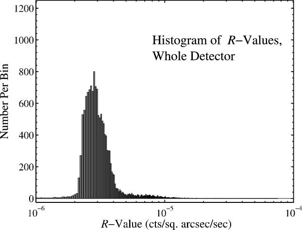
Figure 1: Histogram of the result of 20,000 random samples of the spatial variability of the D–band background. The number of samples in each $\mathcal{R}$–bin is plotted. The bin–size is $2\times 10^{-7}$ counts per square arcsecond per second. The mode, median, and mean values in this histogram are consistent with other measures of the background.

Ultimately, because of the spatial variability of the background, which is evident in Figure 1, the most useful description of the background is probably the local one. The top panel of Figure 2 shows the number of counts by which each of the 21 groups in our sample is brighter than its estimated local background, plotted against redshift. The bottom panel of that figure shows the surface brightness above the local background $SB_{g}$, again plotted against redshift. The 1–$\sigma$ error bars are computed on the ordinates as the summation in quadrature of the $N^{1/2}$ Poisson noise from the group ($\sigma_{g}$) and from the background ($\sigma_{BG}$). No group is seen more than $5\sigma$ above the background, which is our minimum criterion for detection. The dashed line in each panel represents the average value of the quantity on the ordinate of that panel, weighted by the product of the number of pixels and the effective exposure time.

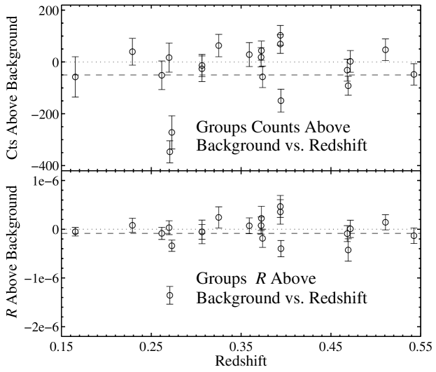
Figure 2: Groups intensities above background in D–band (0.2–1.0 keV). Top Panel: Counts in groups above estimated local background. Bottom Pannel: Surface brightness of groups above background, in units of $\mathcal{R}$–value – i.e., counts per square arcsecond per second. None of the groups is seen more than $5\sigma$ above the background, which is our minimum criterion for detection. The dotted line in each panel is the zero line. The dashed line in each panel represents the weighted average value of the quantity on the ordinate of that panel.

In those cases where both the X–ray and the optical centers of low luminosity groups are known, the correlation between the two shows considerable variance (Mulchaey, 2000). Because of the possibility that the X–ray centers might not coincide with the optical centers of the groups in our survey, we paid particular attention to the analysis with an aperture of radius 500 kpc around each group, because an aperture this size should be large enough to capture a large fraction of the X–rays even if there is an offset of $\sim 0.5\arcmin$ between the X–ray center and the reported optical center. Inasmuch as no group had an $\mathcal{R}$–value $5\sigma$ or more above the local background, the results were substantially the same (no plot shown). Moreover, a greater fraction of groups had negative $SB$–values than when the $250{\rm~{}kpc}$ radius apertures were used ($15/21$ vs. $11/21$).

We finally note that the groups might potentially contaminate the local background estimator. Using reasonable models for the intensity and the spatial distribution of emission from groups, described in detail in § 5.2 below, we estimate that $\geq 30\%$ of flux comes out within our aperture, and $\leq 10\%$ of flux comes out in the annulus from 1.05 to 1.20 times the aperture radius. This portion of group flux that falls within the annulus that we use to define the local background ought to increase the local background measurements, and therefore to depress the surface brightness measurements. The depression, however, is not severe: since the group surface brightness profile is expected to peak toward the center, the surface brightness is still expected to be positive. Moreover, the average $\mathcal{R}$–value of the local background samples was $2.9\times 10^{-6}{\rm~{}cts~{}arcsec^{-2}~{}s^{-1}}$, which is only slightly more than the modal $\mathcal{R}$–value of the randomly placed apertures, and slightly less than their median value. It therefore does not appear that the local background estimator was significantly increased by flux from the groups.

As a final test of whether the estimate of the background was contaminated by group–flux, we used an annulus farther from the aperture: the annulus from 1.5 to 2.0 times the aperture radius. This change had no important effect on our results.

4 Spectral Analysis

We also explored whether examining the shape of the X–ray spectrum would enhance the contrast to the background in the search for groups. In the simplest possible test, we investigated whether the spectral energy distribution (SED) of photons received from the locations of groups differed from that of photons from elsewhere. The background consists of the particle background, and the combined diffuse glows of our galaxy, the Galactic halo, the local group, and extragalactic point–sources and diffuse sources (McCammon & Sanders, 1990; McCammon et al., 2002).

Spectral results from our observations are presented in Figure 3. In our data, the spectrum of the groups is indistinguishable from that of the background. This can be seen in several ways. The top panel of Figure 3 show, with a bin–size of $10{\rm~{}eV}$, the stacked spectrum of the groups in blue, the spectrum of the background in green, and the “rest–framed” spectrum of the groups in red (that is, the energy of each photon from the groups is multiplied by $(1+z_{\rm group})$ prior to binning). The groups and the background both show broad emission features centered at $\sim 0.55{\rm~{}keV}$ and $\sim 1.5{\rm~{}keV}$ (top panel of Figure 3), that are most likely due to O VII at redshift 0 and neutral Si on the detector, respectively. The difference spectrum, however, is 0 to within the 1–$\sigma$ error bars (bottom panel), indicating that the SED from regions of groups is identical to that of other regions. Furthermore, the rest–framed groups spectrum shows no signs of any spectral features.

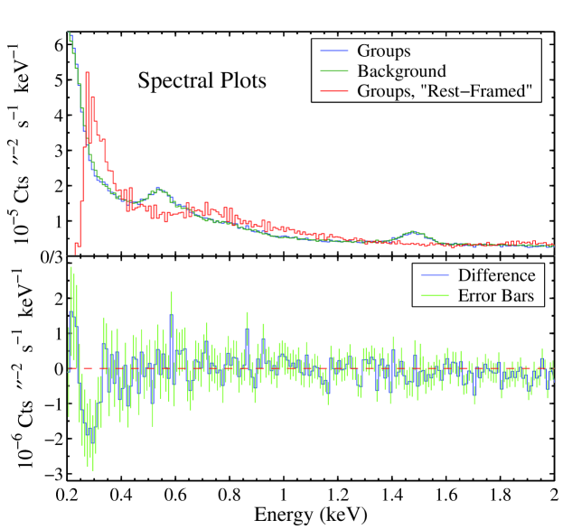
Figure 3: Spectra showing $\mathcal{R}$–values per 10 eV bin.. The rest–framed groups show no signs of any spectral features Top Panel: Groups, background, rest–framed groups spectra, 0.2–2 keV. Spectrum for locations of groups is in blue, for background is in green, and for rest–framed groups is in red. Bottom Panel: Difference spectrum, 0.2–2 keV. 1–$\sigma$ error bars are in green.

5 Discussion

In recent years, research efforts have increasingly been devoted to characterizing the extended X–ray emission from collapsed halos of a variety of masses, from clusters to groups to galaxy–mass halos. For two examples (among many) of studies of gas in higher–mass systems – clusters, Akahori & Masai (2005) investigate the $L_{X}$–$T_{X}$ scaling relation describing intracluster gas, and Arnaud, Pointecouteau, & Pratt (2005) investigate the $M$–$T$ scaling relation of intracluster gas.

Our study is concerned with the properties of gas in lower–mass systems. Xue & Wu (2000) attempt to bridge the gap between clusters and groups in the local universe by performing an analysis of the $L_{X}$–$T$, $L_{X}$–$\sigma_{v}$, and $\sigma_{v}$–$T$ relations of 66 groups and 274 clusters taken from the literature. The XMM–Large Scale Structure survey identified groups and clusters out to redshift 0.6 and beyond, and Willis et al. (2005) examine the $L_{X}$–$T_{X}$ relation of the objects in their survey. Interestingly, in contrast to the analysis in this paper, they detect X–ray emission from low–mass objects out to $z=0.558$. The groups that they found were X–ray selected, so the selection effect surely contributed to their finding groups in their survey while we did not in ours (although we note that this does not explain the physical difference that is responsible for the discrepancy in X–ray luminosities).

5.1 Fits to $L_{X}$–$\sigma_{v}$ Data

In order to estimate how our data ought to have appeared, we need to know what X–ray luminosity should be expected from a group with a given mass or velocity dispersion. The groups of the M03 catalog are a convenient sample of nearby groups with known velocity dispersion and X–ray luminosity. Since any fit to the $L_{X}$–$\sigma_{v}$ relation in the M03 groups will show scatter, a fit is not a line or curve but a 2-dimensional region in $L_{X}$ versus $\sigma_{v}$ space.

In fact, properly, one would want to construct a 2D probability distribution function on $L_{X}$–$\sigma_{v}$ space based on the distribution of the M03 sample. This function would give the probability density for a group drawn from the same population as the reference sample to have a particular velocity dispersion and X–ray luminosity. One could then properly examine the likelihood that the CNOC2 groups are drawn from the same population as the M03 groups.

In practice, it would be difficult to construct the 2-D distribution function we require, because the M03 sample is not dense enough in $L_{X}$–$\sigma_{v}$ space. We therefore reverted to a conventional parametric analysis, based on linear fits to $(\log\sigma_{v},\log L_{X})$ data. We will present several linear fits to the M03 data, and we describe in detail our choice for which linear fit is most appropriate.

PT04 examine the relationship between the X–ray luminosity ($L_{X}$) and the velocity dispersion ($\sigma_{v}$) of galaxy groups in the M03 catalog. They perform regression analysis on $\log L_{X}$ and $\log\sigma_{v}$ and find that, as with any regression in which there is significant scatter, which line is considered the best–fit depends on which variable is considered to be independent and which dependent. We repeated their analysis of the M03 groups and obtained best–fit lines that are very similar (though not identical) to those that they obtained. In this paper, we present our own fits to the data. If velocity dispersion is taken to be the independent variable, the best–fit regression line is

$$\log\left(L_{X}/1{\rm~{}erg~{}s^{-1}}\right)=36.8+2.08\log\left(\sigma_{v}/1{\rm~{}km~{}s^{-1}}\right).$$ (5)

If, on the other hand, luminosity is taken to be the independent variable, the best–fit regression line (what PT04 refer to as the “inverse regression line”) is

$$\log\left(L_{X}/1{\rm~{}erg~{}s^{-1}}\right)=30.9+4.50\log\left(\sigma_{v}/1{\rm~{}km~{}s^{-1}}\right).$$ (6)

Data from M03 and best–fit lines are displayed in Figure 4.

Which regression represents the “true” relation between the X–ray luminosity and the velocity dispersion of groups of galaxies? In Appendix I, we present a more detailed analysis of the relative merits of various procedures for fitting lines to data. The result of this analysis is that neither direct nor inverse regression is ideal, because surely the measurements of both $\sigma_{v}$ and $L_{X}$ were subject to errors, and furthermore there is undoubtedly intrinsic scatter in the $L_{X}$–$\sigma_{v}$ relation. The better relation out of these two is the one in which the variable taken to be independent has lower relative uncertainty. In our case, this is probably the inverse regression, because a velocity dispersion determined from only a few galaxies is likely to be quite uncertain. Furthermore, the steeper (inverse) relation comes closer to fitting the high–$\sigma_{v}$, high–$L_{X}$ end of the distribution of groups, which is the end that we are most interested in when looking for groups at $z\sim 0.5$. Still, although the inverse regression is probably preferable to the direct regression, since there is scatter in both variables, this situation calls for least squares orthogonal distance fitting (described in Appendix I). If we assume that the typical relative errors on $\log(\sigma_{v})$ and $\log(L_{X})$ are the same (i.e., the error is shared equally between the two variables), then the distance–fit line,

$$\log\left(L_{X}/1{\rm~{}erg~{}s^{-1}}\right)=31.5+4.25\log\left(\sigma_{v}/1{\rm~{}km~{}s^{-1}}\right),$$ (7)

is nearly as steep as the inverse regression line, as shown in Figure 4.

5.2 Limits on Group Luminosities

Since none of the groups was visible at $5\sigma$ above the background, we may place limits on their fluxes and therefore, since we know their redshifts, on their luminosities. The total number of background counts $TC_{BG}$ at the location of a group is estimated from the smoothed background image. Assuming Poisson statistics, the standard deviation on this number is $\sigma_{TC_{BG}}=(TC_{BG})^{1/2}$. The maximum number of group counts $TC_{G}$, then, is limited by

$$TC_{G}<5\sigma_{TC_{BG}}=5\sqrt{TC_{BG}},$$ (8)

We estimate each group’s temperature with the standard relation given in, e.g., Mulchaey (2000):

$$T=\frac{m_{p}}{\mu}\sigma_{v}^{2}\times(k\beta),$$ (9)

where $m_{p}$ is the proton mass, $\mu$ is the mean molecular weight, $k$ is Boltzmann’s constant, and $\beta$, whose empirical value tends to be around $2/3$, is the eponymous parameter of the isothermal–$\beta$ model for density and may be considered to be defined by this equation. (For low-density objects, $\beta$ has been measured to be closer to $1$, but for analytical simplicity we used $\beta=2/3$ for most calculations.) The $\beta$ density model for a spherical isothermal plasma is

$$\rho(r)=\rho_{0}\left(1+\left(\frac{r}{r_{c}}\right)^{2}\right)^{-3\beta/2},$$ (10)

where $\rho_{0}$ is the central density, $r$ is the radial distance from the sphere’s center, and $r_{c}$ is the “core radius,” a distance within which the density is nearly constant (approximately $\rho_{0}$). Using the Astrophysical Plasma Emission Code (APEC) model in XSPEC, we solve for what X–ray luminosity, at a given temperature, would lead to the number of group counts given by the maximum possible value of $TC_{G}$ in (8).

In Figure 4, the X’s show the maximum luminosity that each group could have had during our observations (if the group were more luminous, it would have shown up at $>5\sigma$ above the background). If a group is predicted to be less luminous than the luminosity represented by its X, then it is no surprise that we failed to see the group; conversely, if a group is predicted to be more luminous than the luminosity represented by its X, then the group is less luminous than predicted. The dashed line shows the $L_{X}$–$\sigma_{v}$ direct regression line, the dashed–dotted line shows the inverse regression line, and the solid line shows the distance–fit line. All X’s (all groups) lie above the direct regression line, so if that line represents the true relationship between the variables, there is no surprise in seeing none of the groups. Three groups, however, lie below both the inverse regression line and the distance–fit line; so if those lines represent the true relationship between the variables, it might be surprising that we failed to see three of the groups. In the remainder of this section, we will try to quantify how surprising it is.

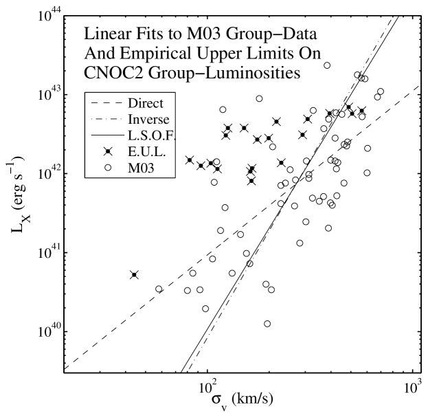
Figure 4: Linear Fits to M03 Group–Data And Empirical Upper Limits On CNOC2 Group–Luminosities: bolometric X–ray luminosity vs. line–of–sight velocity dispersion. The circles show the M03 groups. The dashed line is the direct regression line, the dashed–dotted line is the inverse regression line, and the solid line (L.S.O.F.) is the least squares orthogonal fit line. These three lines are fits to the M03 data. The X’s (E.U.L.) display the “empirical upper limits” to groups’ luminosities, i.e., the maximum luminosities that the CNOC2 groups could have had during our observations without showing up at more than $5\sigma$ above the background. The uncertainty in velocity dispersion associated with the X’s is typically nearly $\sim 100\%$, as shown in Table 1. Three of the X’s lie beneath both the dashed–dotted and the solid lines, indicating that these three groups were predicted to be luminous enough to be detected, and yet were not.

5.3 Quantifying Surprise

The CNOC2 catalog of small groups (Carlberg et al., 2001b) contains groups with as few as three galaxies in them. Any measurement of the velocity dispersion of such a group will necessarily have large uncertainties. In fact, for some groups, the estimated uncertainty in velocity dispersion is actually greater than the velocity dispersion itself. Because the symbol $\sigma$ is frequently used to denote both uncertainty and velocity dispersion, it is inelegant to represent the uncertainty in velocity dispersion, but, eschewing elegance, we shall use $\sigma_{\sigma_{v}}$ to denote uncertainty on $\sigma_{v}$.

It is possible that our null result – our failure to detect any of the groups in our survey – occurred because the velocity dispersions of the three groups predicted to be observed were overestimated. If so, then perhaps their predicted luminosities based on, e.g., (7), should have been low enough that the groups should not have been seen after all. Of course, if there were no bias to the measurements of $\sigma_{v}$, it is just as likely that the velocity dispersions of these three groups were underestimated, which would make their non–detection even more surprising. Furthermore, in order for this sort of statistical error to explain our null result, not only would the velocity dispersions of the three groups that we think we ought to have detected need to have been sufficiently overestimated, but no other groups could have have had their velocity dispersions underestimated by too much. In short, the statistical errors would need to be in particular directions on particular groups. If there is no non–statistical reason for measurements to be in error, then what is the likelihood that the types of error needed to explain our null result actually occurred?

To answer this question, we simulated 10,000 mock–CNOC2 catalogs, each with its own set of mock–velocity dispersions ($\{\widehat{\sigma_{v}}(i)\}$) associated with the mock–groups. If the set of measured velocity dispersions from the actual CNOC2 catalog is $\{\sigma_{v}(i)\}$, then, for each mock–catalog, the simulated velocity dispersion of the $i$th group $\widehat{\sigma_{v}}(i)$ was drawn from from a gamma distribution with mean $\sigma_{v}(i)$ and standard deviation $\sigma_{\sigma_{v}}(i)$. The gamma distribution has the attractive property that the mean and the standard deviation may be independently specified. Because the tail of the gamma distribution extends to infinity, however, a small fraction of mock–groups were initially given unrealistically high velocity dispersions. Incidentally, this is preferable to the normal distribution, which has another tail that extends below zero to negative infinity – unphysical values for velocity dispersion. To deal with the gamma distribution’s problem of predicting a few unrealistically high values, we, for each group $i$, eliminated from the set of mock–catalogs all mock–groups with velocity dispersions more than $4\sigma_{\sigma_{v}}(i)$ above the mean ($\sigma_{v}(i)$), and replaced these values with new gamma–distributed variables. We repeated this procedure iteratively until there were no more mock–groups with velocity dispersion more than $4\sigma_{\sigma_{v}}$ above the mean. Because this procedure involves replacing the high–end outliers with values closer to the mean, it had the effect of slightly depressing the mean. All values were therefore increased by the difference between the new mean and $\sigma_{v}(i)$, thereby raising the mean back to $\sigma_{v}(i)$, as it should be.

We also tried several other random distributions for assigning mock–velocity dispersions to our mock groups. We tried a gamma distribution with no high–end cut–off; and we tried several modifications of the normal distribution, all of which included a low–end cut–off at $0$. We found that those results were not importantly different from results from the gamma distribution with the high–end cut–off, which is the analytically simplest distribution that produces realistic results. Results are presented only for the mock–catalogs generated with the high–end cut–off gamma distribution.

Each mock–group was assigned the same aperture size as the corresponding real group. Its mock–intensity was spatially distributed according to a spherical isothermal–$\beta$ model. Since emissivity is proportional to the square of density $\rho$, the surface brightness or intensity $I$ is proportional to the integral along the line–of–sight of $\rho^{2}$. At a projected viewing “impact parameter” $b$ from the sphere’s center,

$$I(b)\propto\int_{r=b}^{r=r_{h}}\rho(r)^{2}{\rm d}s,$$

where $r_{h}$, the “halo radius,” is the outer boundary of the sphere of plasma, and $s$ is the variable along the line–of–sight. Substituting for $\rho$ with equation (10) and performing the integration results in the following expression for the surface brightness:

$$\mathcal{B}(x,A,\beta)\propto(1+x^{2})^{-3\beta}(A^{2}-x^{2})^{1/2}\mbox{ }{{}_{2}F_{1}}\left(\frac{1}{2},3\beta,\frac{3}{2},\frac{x^{2}-A^{2}}{1+x^{2}}\right),$$ (11)

where $x\equiv b/r_{c}$ and $A\equiv r_{h}/r_{c}$ are substitutions to simplify the integration, and ${}_{2}F_{1}$ is the Gauss hypergeometric function. Three quantities go into the normalization of $\mathcal{B}$ for each mock–group: its mock–luminosity from e.g. (7); its luminosity distance $D_{L}(z)$; and its core radius. Finally, we assumed a foreground column density of neutral hydrogen of $2\times 10^{20}{\rm~{}cm^{-2}}$ (Dickey & Lockman, 1990).

It was unclear what core radii our mock–groups should be assigned, because the $\beta$-model core radii of groups and clusters vary a great deal. Ota & Mitsuda (2004) report that in a sample of 79 clusters, including 45 “regular” clusters and 34 “irregular” clusters, the mean of all 79 values of $r_{c}$ is $(163\pm 202)~{}{h_{70}}^{-1}{\rm~{}kpc}$, midway between the mean $r_{c}$ of the regular clusters ($(76\pm 60)~{}{h_{70}}^{-1}{\rm~{}kpc}$) and the mean $r_{c}$ of the irregular clusters ($(273\pm 259)~{}{h_{70}}^{-1}{\rm~{}kpc}$). Because there is no strong correlation between $r_{c}$ and group–mass, we think it is reasonable to adopt a uniform assumed value of $r_{c}$ for the mock–groups in our mock–catalogs. We ultimately decided to set each mock–group’s core radius to $125{\rm~{}kpc}$, because this value lies in the middle of the range of values reported by Ota & Mitsuda (2004). So long as the value of $r_{c}$ that we adopted is physically plausible, the precise value does not matter much, because the predicted number of counts from a group, within an aperture of fixed size, is not very sensitive to the assumed value of $r_{c}$, as long as the angular–size of the aperture is larger than that of the core radius.

The SED of each mock–group (and hence the flux in a given energy band) is calculated with XSPEC, using APEC, with its mock–temperature calculated from equation (9). For $A$, we tried values between $2$ and $\infty$, and for $\beta$, we tried values between $0.6$ and $1.0$. The results presented below are for $A=\infty$ and $\beta=2/3$, and for D–band (0.2–1.0 keV).

In brief, the results of this Monte Carlo indicate that the probability appears to be small, but not vanishingly so, that statistical fluctuations in the measured values of $\sigma_{v}$ explain our null result. Figure 5 shows a summary of the mock–catalog results. The median and the mode number of groups seen per catalog are both $3$, and the mean number seen is $3.1$, which is in good agreement with the prediction of section 5.2. The finding of our observation – that no groups were seen – occurred in only $3.5\%$ of the mock–catalogs. If there were no systematic errors in the measurements of velocity dispersions of the CNOC2 groups, then it is unlikely but not impossible that the only reason we had expected some of the groups to be visible in the first place was erroneously high measurements of $\sigma_{v}$.

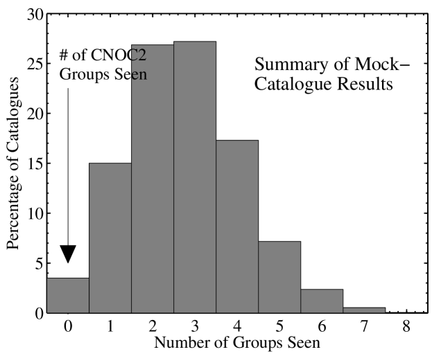
Figure 5: Histogram of the results of the mock–catalog analysis. Of the 10,000 mock–catalogs, $96.5\%$ contained at least 1 mock–group visible at the $5\sigma$ level. In the actual CNOC2 survey no groups were visible at this level.

5.4 Redshifted Mulchaey Groups

Perhaps we have placed too much emphasis, in sections 5.1 and 5.2, on which best–fit line actually fits the M03 data the best – when the truth is that there will be significant scatter to the data around any line drawn through the cloud of points. An alternative way to determine whether it is surprising that no groups in our survey showed up at $5\sigma$ above the background is to ask whether the CNOC2 groups and the M03 groups were drawn from the same population. We addressed this question by investigating how many of the groups in the M03 atlas would have been visible at the $5\sigma$ level if they had been in our observation.

The M03 groups are all in the local universe, approximately at redshift 0. If they had been in our survey, i.e., between redshifts 0.1 and 0.6, they would have both been dimmer and subtended a smaller solid angle on the sky. Furthermore, they would have been observed with XMM–Newton, which, owing to its greater focal ratio, has a higher particle background rate than ROSAT (the instrument with which they were originally observed).

There were 109 groups in the M03 catalog, of which 61 were seen in X–rays. We simulated observations of each of these 61 M03 groups at each of the 21 redshifts of the CNOC2 groups, ranging from $z_{1}=0.165$ to $z_{21}=0.543$ (ID numbers taken from Table 1). As before, our criterion was that a group must outshine the background by at least $5\sigma$ to qualify as being detected in our simulated observations. Each group was assumed to be at a location with detector–averaged characteristics: the mean exposure map value, the median background value (from Figure 5), the mean amount of smearing due to the point–spread function, and the mean amount of lost usable detector–area because of bright point sources. Much like in the mock–catalog calculations described in section 5.3, we calculated the count–rate of each group with XSPEC, using APEC, with the group’s temperature calculated from equation (9). We distributed emission according to the isothermal–$\beta$ profile using equation (11), with $\beta=2/3$, $A=\infty$, and $r_{c}=125{\rm~{}kpc}$. For our simulated observations, we used an aperture of $250{\rm~{}kpc}$, and looked in D–band. For background, we used $\mathcal{R}_{BG}=3.0\times 10^{-6}{\rm~{}cts~{}arcsec^{-2}~{}s^{-1}}$. Finally, as before, we assumed a foreground column density of neutral hydrogen of $2\times 10^{20}{\rm~{}cm^{-2}}$. Within our simulation, the number of M03 groups that exceeded the $5\sigma$ detection criterion varied from 22 of the 61 total groups (or $p_{1}=36\%$) at the lowest redshift ($z_{1}$), to 2 of 61 ($p_{21}=3\%$) at the highest redshift ($z_{21}$).

We identify two populations of the Mulchaey groups – all 109, and the 61 that were seen in X–rays. In Appendix II, we present in detail our estimate of the likelihood that the CNOC2 groups and the M03 groups were drawn from the same population. The result is that the probability of obtaining our null result on the assumption that the CNOC2 groups were drawn from the same population as the whole M03 catalog is 14.7%; and the analogous probability on the assumption that the CNOC2 groups were drawn from the same population as the 61 X–ray–bright M03 groups is 2.8%. These probabilities (especially the latter) are low enough to be interesting, but are certainly not dispositive.

6 Conclusion

The analysis in section 5.4 is mildly suggestive that the groups of the CNOC2 survey constitute a sample that is on average less luminous than the sample of groups observed by Mulchaey and collaborators in the 2003 atlas. The interesting comparison, however, is not between two particular samples, but rather between the population of groups at intermediate redshift and the population in the local universe.

A first caveat is that the two samples were selected in very different ways, and there is no a priori reason to suspect that their underlying populations have similar luminosity functions. Furthermore, it is conceivable that for some reason the M03 groups should be expected to be a more luminous sample of their population than the CNOC2 groups are of theirs. Perhaps the M03 groups are on average more massive (although the ranges and distributions of velocity dispersions for the two samples are nearly identical). Do the M03 groups contain more galaxies than the CNOC2 groups? Certainly, Mulchaey reports more galaxies per group on average – including as many as 63 galaxies in one group. Of the CNOC2 groups in our field of view, none contained more than 4 galaxies with identified redshifts. But most or all of the difference here is almost certainly due to the difficulty of measuring spectroscopic redshifts of faint galaxies at large distances; we therefore see no reason to think that the M03 groups are on average more massive than the CNOC2 groups.

An obvious criticism of the present work is that the CNOC2 groups might not be groups at all, but just chance superpositions of galaxies. While this would clearly explain the lack of X–ray emission, we will argue that we find it unlikely to be the reason why we detected no hot gas.

Carlberg et al. (2001b) identified as a group any object in the CNOC2 Survey that contains at least 3 galaxies in sufficiently close redshift–space proximity. This identification procedure does leave open the possibility of confusion: if two galaxies are separated by a large distance, but have appropriately large peculiar velocities, they could have similar recessional velocities (redshifts) despite not being part of a gravitationally bound structure. Or, even if a few galaxies are close to one another in physical space, they will not be part of a bound system without a dark matter halo that is massive enough to bind them.

In searching for groups and clusters, it is often assumed that where there are associations of galaxies, there is dark matter to bind them, but this assumption could be wrong. With rich clusters, there are multiple independent checks of this assumption: the temperature of intergalactic gas (which can be detected through its X–ray emission or through inverse Compton distortions to the cosmic microwave background) is one indicator of the mass; the velocity–distribution of galaxies is another indicator of the mass, and in particular the distribution should be Maxwellian (or Gaussian) for a virialized structure; and the degree of gravitational lensing of background galaxies is a third indicator of the mass.

The first check has obviously failed in this case – for these 21 groups, there is no apparent hot gas component. The second check is useless for an association of very few (3–6) galaxies – nearly any velocity distribution is consistent with an underlying Gaussian distribution. How about lensing? For structures of $\;\hbox to0.0pt{\lower 2.5pt\hbox{$\sim$}\hss}\raise 1.5pt\hbox{$<$}\;10^{13.5}M_{\sun}$, noise prevents detection of a lensing signal. As a result, in the CNOC2 fields, it is only possible to determine a statistical lensing mass for the groups by stacking them and determining their combined lensing signal. This analysis has been performed by Hoekstra et al. (2001, 2003): their calculated estimate of the average velocity dispersion per group based on the mass inferred from the average shearing of background galaxies ($258_{-56}^{+45}{\rm~{}km~{}s^{-1}}$ for $\Omega_{m}=0.2$ and $\Omega_{\Lambda}=0.8$) is in good agreement with the average velocity dispersion of $230{\rm~{}km~{}s^{-1}}$ from the kinematics of the groups’ member–galaxies. The observed lensing signal was sufficiently strong that chance projections of unbound galaxies alone would have difficulty mimicking it. Some of the detected lensing mass is therefore almost surely in the form of galaxies orbiting within a parent dark matter halo – groups. It is entirely reasonable to expect part of this group–component of the lensing mass to consist of hot gas trapped within the group potential. On the other hand, it is not unlikely that a portion of the lensing mass is in the form of projected, yet physically unassociated, galaxies. Although there may be limited amounts of gas associated with the individual galaxies, such projections will produce no extended group emission. Therefore, the presence of a lensing signal does not automatically lead to the expectation of group–like X–ray emission that is at sufficient surface–brightness to be detectable in our survey.

It is conceivable that there were several relatively massive groups, or dark clusters (i.e., cluster–mass objects with very low mass–to–light ratios), that dominated the mean mass measurement. Although we cannot rule out the possibility that a large fraction of the mass is in only a few objects that happened to fall outside the field of view of our observations, and that the remaining objects are not gravitationally bound structures but rather chance associations of galaxies that just happen to be near one another in redshift–space, this seems somewhat unlikely: Combinatorial statistics dictate that if there were a few massive halos scattered among the 40 alleged groups and none of the rest are true groups, then the probability is low that all the massive ones ended up among the 19 groups that did not fit into our field of view. Consider, for instance, if there were only four massive halos: since 19 is roughly half of 40, if the four massive halos were randomly distributed the probability that all four would be out of our field of view is $\;\hbox to0.0pt{\lower 2.5pt\hbox{$\sim$}\hss}\raise 1.5pt\hbox{$<$}\;\left(1/2\right)^{4}$. Furthermore, a calculation in Carlberg et al. (2001b) shows that the number of alleged groups in the field in the redshift range $0.1<z<0.6$ (40 in the CNOC2 field, 21 in the EPIC–PN field of view) is roughly consistent with predictions. The concordances both of the observed number of groups with the predicted number, and of the observed velocity dispersions with the mass inferred from weak lensing, together constitute a strong indication that the CNOC2 group sample does not suffer significant contamination from chance superpositions of galaxies. An important caveat is that the number of groups in the CNOC2 fields in the high $\sigma_{v}$ range is in excess of the aforementioned predictions derived from the basic formalism of Press & Schechter (1974) by a factor of $\sim 4$. Based on the Carlberg et al. (2001a) results, $\sim 80\%$ of such high $\sigma_{v}$ groups could be false, and our own null results are consistent with such this hypothesis.

If we take seriously the conclusion, for which our analysis has generated some modest evidence, that galaxy groups at intermediate redshift are less X–ray luminous than those at redshift zero, we can think of several potential explanations. Groups at $z\sim 0.5$ are younger than their relatives in the local universe, which leads to the following three possibilities: $(i)$ Since simulations and observations indicate that groups and clusters at the present are accreting gas from cosmic filaments, groups at a younger stage of the universe would presumably have been accreting gas for less time than the more evolved groups of the present–day universe and might therefore contain less gas. $(ii)$ Even if the intragroup gas in young groups is not lower density than the gas in groups today, if the young groups are still in the process of heating up – if they have not yet reached their virial temperatures – their luminosities would be reduced. (We find this possibility to be unlikely, because the heating timescale is short relative to a Hubble time, even at $z\sim 0.5$.) $(iii)$ Even if the gas in young groups is on average the same density and the same temperature as the gas in nearby groups, if it is of lower metallicity its X–ray emissivity would be reduced. There are undoubtedly feedback processes that enrich the intragroup medium, and pristine gas of primordial abundance is also surely constantly falling onto groups, so it is not clear whether to expect higher metallicity in the IGM of groups that are at $z\sim 0.5$ or at $z\sim 0$. For warm gas, observed in a soft X–ray band such as our D–band, line–emission can be important, depending on abundances. For example, if a $T=1{\rm~{}keV}$ group at redshift 0.5 contained primordial gas, its D–band X–ray flux would be only two thirds as great as if its gas were at 10% solar abundance and only half great as if its gas were at 20% solar abundance. It is possible, therefore, that the relation between velocity dispersion and X–ray luminosity ought to be shifted down by a factor of $\sim 2$ in Figure 4. Such a shift would make it less surprising that we detected no X–ray emission from the groups.

Future data on high–redshift clusters that make it possible to examine the time–evolution of the density and metallicity of the intracluster medium in low–mass clusters, and deeper searches for X–ray gas in low–mass objects at intermediate redshift, will help to answer why our survey failed to detect such gas.

We thank Kevin Roy Briggs and Maurice Leutenegger for invaluable advice on reduction and analysis of XMM–Newton data; and we thank Fred Blumberg for extremely helpful comments and criticism. We furthermore would like to acknowledge the many incisive observations and constructive suggestions from our referee and from our scientific editor. FP acknowledges support by NASA through grant NAG5-13354, and CAS acknowledges support by NASA grant SAOG03-4158A. This research has made use of publicly available data from the XMM-Newton Science Archive.

Appendix I

In this Appendix, we address the question of which regression represents the “true” relation between the velocity dispersion and the X–ray luminosity of groups of galaxies. It is instructive first to consider a statistical effect that is common to all regression analysis. It has been known at least since Karl Pearson’s seminal paper in 1901 that if there is scatter (say, due to measurement error) in the variable considered to be the independent one, this will in general cause the recovered slope from regression analysis to be shallower than the slope of the true underlying relation between the variables. (PT04 demonstrate a nice example of this effect.) An important consequence of this effect is that when there is scatter in both variables, the slopes from both the direct and the inverse regression will be shallower than the respective true slopes.

For example, suppose two variables $x$ and $y$ are related by $y=\alpha x$ (or $x=\beta y$, where $\beta=1/\alpha$). In an experiment, a large number of $(x,y)$ pairs are measured, and there are statistical uncertainties in the measurements of both variables. If $x$ is considered to be the independent variable, regression analysis will lead to $y=\hat{\alpha}x$, where in general $\hat{\alpha}<\alpha$ because of the scatter in $x$. If $y$ is considered to be the independent variable, regression (“inverse regression”) analysis will lead to $x=\tilde{\beta}y$, where in general $\tilde{\beta}<\beta$ because of the scatter in $y$. Of course, if we wish to represent $y$ as a function of $x$ even in the case of the inverse regression, we will write $y=\tilde{\alpha}x$, where $\tilde{\alpha}=1/\tilde{\beta}>\alpha$. So, although the recovered slopes are in general less than the respective true slopes for both regressions ($\hat{\alpha}<\alpha$ and $\tilde{\beta}<\beta$), when we fix the abscissa and ordinate variables we get a shallower slope than the true one in the case of the direct regression and and a steeper slope in the case of the inverse regression. Note that this effect holds whether the scatter comes from measurement error or is intrinsic to the variables.

When there is scatter in both variables, so that neither one is a proper independent variable, it is sometimes appropriate to use a type of best–fit line that depends on the geometric orientation of the points. Instead of finding the line that minimizes the summed, squared vertical deviations of the data from the line, as in the case of regression, some situations are better analyzed by finding the line that minimizes the summed, squared perpendicular distances of the data from the line. This is sometimes called “least squares orthogonal distance fitting,” and was the subject of Pearson (1901). Because this type of fitting, in contrast to linear regression, is unfortunately sensitive to the units of measurement, it is advisable to normalize the data prior to fitting. The most common normalization is by the estimated errors or uncertainties ($\sigma_{x}$ and $\sigma_{y}$) on the variables (Press et al., 1992; Akritas & Bershady, 1996). The direct regression line will have the minimum slope, the inverse regression line will have the greatest slope, and the “distance–fit” line will have an intermediate slope (closer to the direct regression slope if the scatter in $x$ is smaller; closer to the inverse regression slope otherwise). All three lines intersect at the centroid of the data.

For completeness, we present the equation of the least squares orthogonal distance fit line. Let us express the measured data as a set of $N$ points $\{(x_{i},y_{i})\}_{i=1}^{N}$. To simplify the form of the line’s equation, we define the following sums of data:

$$S_{x}\equiv\sum_{i=1}^{N}x_{i}\qquad S_{y}\equiv\sum_{i=1}^{N}y_{i}$$

$$S_{x^{2}}\equiv\sum_{i=1}^{N}{x_{i}}^{2}\quad S_{xy}\equiv\sum_{i=1}^{N}(x_{i}\>y_{i})\quad S_{y^{2}}\equiv\sum_{i=1}^{N}{y_{i}}^{2};$$ (12)

and we define the following combinations of these sums:

$$A \equiv S_{x}S_{y}-NS_{xy}$$

$$B \equiv (S_{x})^{2}-(S_{y})^{2}-N(S_{x^{2}}-S_{y^{2}})$$

$$C \equiv -S_{x}S_{y}+NS_{xy}.$$ (13)

If the equation of the least squares orthogonal distance fit line is

$$y=mx+b,$$ (14)

then the slope of the line is given by

$$m=\frac{-B\pm\sqrt{B^{2}-4AC}}{2A},$$ (15)

and the $y$–intercept is given by

$$b=\frac{S_{y}-mS_{x}}{N}.$$ (16)

The expression for $m$ in equation (15) contains a $\pm$–sign from the solution to a quadratic equation. One solution for $m$ gives the line that minimizes the summed squared orthogonal distances to the points, and the other solution gives the line passing through the centroid of the data that maximizes the summed squared orthogonal distances to the points.

Appendix II

In this Appendix, we address how to compute the probability that the CNOC2 groups and the Mulchaey (M03) groups derive from the same population. In order to do this, we find the properties of the hypothetical parent group population $\mathcal{P}$ that maximize the joint probability of our results and Mulchaey’s results.

Let the redshifts of the CNOC2 groups be labeled $\{z_{k}\}_{k=1}^{21}$. At each redshift $z_{k}$, let $N_{k}$ be the number of M03 groups that our simulation predicts would have been visible in our 110 ksec observation, and let $p_{k}$ be the probability that a group drawn from $\mathcal{P}$ will be visible in our survey if it is in our field of view and at redshift $z_{k}$.

At redshift $z_{k}$, the probability of obtaining our result – of not seeing any groups – is

$$q_{k}\equiv(1-p_{k});$$ (17)

and the probability of obtaining the M03 result – of seeing $N_{k}$ groups, as predicted by our simulation – is

$$B(M,N_{k},p_{k})={M\choose N_{k}}{p_{k}}^{N_{k}}{q_{k}}^{M-N_{k}},$$ (18)

where $M$ is the total number of groups in the M03 sample, either 109 or 61, as described above.

The joint probability, then, of obtaining our result and of obtaining the M03 result is

$$P_{\rm joint}(z_{k})=q_{k}B(M,N,p_{k})={M\choose N_{k}}{p_{k}}^{N_{k}}{q_{k}}^{M-N_{k}+1}.$$ (19)

At each redshift $z_{k}$, we find the binomial probability $\hat{p}_{k}$ that maximizes $P_{\rm joint}(z_{k})$. This set of optimal probabilities $\{\hat{p}_{k}\}$ can be thought of as defining the parent population $\widehat{\mathcal{P}}$ of groups that maximizes the probability that we would obtain our null result and that the M03 groups would have their observed properties. Each percentage $\hat{p}_{k}$ in turn can be thought of as an estimate of the probability that a group would be visible in our survey if it were randomly selected from $\widehat{\mathcal{P}}$ and placed at redshift $z_{k}$. The value $\hat{q}_{k}\equiv(1-\hat{p}_{k})$, then, is the probability that such a group would not be detected in our survey.

If 21 groups were selected at random from $\widehat{\mathcal{P}}$ and placed at the 21 redshifts $z_{k}$, the probability that none would be seen in our survey is the product of the 21 quantities $\hat{q}_{k}$. A maximal estimate of the conditional probability that none of the CNOC2 groups would be detected at the $5\sigma$ level, given that the CNOC2 groups were drawn from the same population as the M03 groups, may therefore be represented as follows:

$$P(\varnothing~{}|{\rm~{}same~{}pop.})\leq\prod_{k=1}^{21}\left(1-\hat{p}_{k}\right),$$ (20)

where $\varnothing$ denotes our null result of not detecting any CNOC2 groups. The result of our simulation is that the product in equation (20) is $P\leq 14.7\%$ for $M=109$ and $P\leq 2.8\%$ for $M=61$; this indicates that the probability is small, but not vanishing, that the CNOC2 groups in our survey have the same luminosity function as the M03 groups.

References

- Akahori & Masai (2005) Akahori, T. & Masai, K. 2005, PASJ, 57, 419
- Akritas & Bershady (1996) Akritas, M. G. & Bershady, M. A. 1996, ApJ, 470, 706
- Arnaud et al. (2005) Arnaud, M., Pointecouteau, E., & Pratt, G. W. 2005, A&A, 441, 893
- Carlberg et al. (2001a) Carlberg, R. G., Yee, H. K. C., Morris, S. L., Lin, H., Hall, P. B., Patton, D. R., Sawicki, M., & Shepherd, C. W. 2001a, ApJ, 563, 736
- Carlberg et al. (2001b) —. 2001b, ApJ, 552, 427
- Dickey & Lockman (1990) Dickey, J. M. & Lockman, F. J. 1990, ARA&A, 28, 215
- Ettori et al. (2003) Ettori, S., Tozzi, P., & Rosati, P. 2003, A&A, 398, 879
- Fang et al. (2006) Fang, T., Gerke, B. F., Davis, D. S., Newman, J. A., Davis, M., Nandra, K., Laird, E. S., Koo, D. C., Coil, A. L., Cooper, M. C., Croton, D. J., & Yan, R. 2006, astro-ph/0608382
- Fukugita & Peebles (2004) Fukugita, M. & Peebles, P. J. E. 2004, ApJ, 616, 643
- Giacconi et al. (1974) Giacconi, R., Murray, S., Gursky, H., Kellogg, E., Schreier, E., Matilsky, T., Koch, D., & Tananbaum, H. 1974, ApJS, 27, 37
- Hoekstra et al. (2003) Hoekstra, H., Franx, M., Kuijken, K., Carlberg, R. G., & Yee, H. K. C. 2003, MNRAS, 340, 609
- Hoekstra et al. (2001) Hoekstra, H., Franx, M., Kuijken, K., Carlberg, R. G., Yee, H. K. C., Lin, H., Morris, S. L., Hall, P. B., Patton, D. R., Sawicki, M., & Wirth, G. D. 2001, ApJ, 548, L5
- Mahdavi & Geller (2004) Mahdavi, A. & Geller, M. J. 2004, ApJ, 607, 202
- McCammon et al. (2002) McCammon, D., Almy, R., Apodaca, E., Bergmann Tiest, W., Cui, W., Deiker, S., Galeazzi, M., Juda, M., Lesser, A., Mihara, T., Morgenthaler, J. P., Sanders, W. T., Zhang, J., Figueroa-Feliciano, E., Kelley, R. L., Moseley, S. H., Mushotzky, R. F., Porter, F. S., Stahle, C. K., & Szymkowiak, A. E. 2002, ApJ, 576, 188
- McCammon & Sanders (1990) McCammon, D. & Sanders, W. T. 1990, ARA&A, 28, 657
- Mulchaey (2000) Mulchaey, J. S. 2000, ARA&A, 38, 289
- Mulchaey et al. (2003) Mulchaey, J. S., Davis, D. S., Mushotzky, R. F., & Burstein, D. 2003, ApJS, 145, 39
- Osmond & Ponman (2004) Osmond, J. P. F. & Ponman, T. J. 2004, MNRAS, 350, 1511
- Ota & Mitsuda (2004) Ota, N. & Mitsuda, K. 2004, A&A, 428, 757
- Pearson (1901) Pearson, K. 1901, Philosophical Magazine, 2, 609
- Plionis & Tovmassian (2004) Plionis, M. & Tovmassian, H. M. 2004, A&A, 416, 441
- Press et al. (1992) Press, W. H., Flannery, B. P., Teukolsky, S. A., & Vetterling, W. T. 1992, Numerical Recipes: The Art of Scientific Computing, 2nd edn. (Cambridge (UK) and New York: Cambridge University Press)
- Press & Schechter (1974) Press, W. H. & Schechter, P. 1974, ApJ, 187, 425
- Rosati et al. (2002) Rosati, P., Borgani, S., & Norman, C. 2002, ARA&A, 40, 539
- Rowan-Robinson & Fabian (1975) Rowan-Robinson, M. & Fabian, A. C. 1975, MNRAS, 170, 199
- Scharf (2002) Scharf, C. 2002, ApJ, 572, 157
- Schwartz (1978) Schwartz, D. A. 1978, ApJ, 220, 8
- Willis et al. (2005) Willis, J. P., Pacaud, F., Valtchanov, I., Pierre, M., Ponman, T., Read, A., Andreon, S., Altieri, B., Quintana, H., Dos Santos, S., Birkinshaw, M., Bremer, M., Duc, P.-A., Galaz, G., Gosset, E., Jones, L., & Surdej, J. 2005, MNRAS, 363, 675
- Xue & Wu (2000) Xue, Y.-J. & Wu, X.-P. 2000, ApJ, 538, 65