Optimising Optimal Image Subtraction

Abstract

Difference imaging is a technique for obtaining precise relative photometry of variable sources in crowded stellar fields and, as such, constitutes a crucial part of the data reduction pipeline in surveys for microlensing events or transiting extrasolar planets. The Optimal Image Subtraction (OIS) algorithm of Alard & Lupton (1998) permits the accurate differencing of images by determining convolution kernels which, when applied to reference images with particularly good seeing and signal-to-noise $(S/N)$, provide excellent matches to the point-spread functions (PSF) in other images of the time series to be analysed. The convolution kernels are built as linear combinations of a set of basis functions, conventionally bivariate Gaussians modulated by polynomials. The kernel parameters, mainly the widths and maximal degrees of the basis function model, must be supplied by the user. Ideally, the parameters should be matched to the PSF, pixel-sampling, and $S/N$ of the data set or individual images to be analysed. We have studied the dependence of the reduction outcome as a function of the kernel parameters using our new implementation of OIS within the IDL-based Tripp package. From the analysis of noise-free PSF simulations of both single objects and crowded fields, as well as the test images in the Isis OIS software package, we derive qualitative and quantitative relations between the kernel parameters and the success of the subtraction as a function of the PSF widths and sampling in reference and data images and compare the results to those of other implementations found in the literature. On the basis of these simulations, we provide recommended parameters for data sets with different $S/N$ and sampling.

1 Introduction

Many astrophysical experiments rely on the precise determination of lightcurves from sources which are either weak, weakly variable, and/or situated in densely populated backgrounds. Prominent examples are the detection of extrasolar planets via the transit technique, gravitational microlensing, and supernova searches. As these events are intrinsically rare, dedicated large-scale surveys have only become feasible due to automated reduction and photometry of large amounts of CCD data. An overview of microlensing surveys (Ogle, Eros, Macho, Moa, and Planets) is given in Dominik et al. (2002) and the references cited therein.

Whenever stellar point spread functions (PSFs) overlap, the determination of the background correction for aperture photometry is difficult at best and heavy blending of stellar profiles renders the assignment of flux to one source or another ambiguous or even impossible. Iterative deblending methods of different kinds have been implemented and are in wide use: photometry packages like Daophot (Stetson 1987) or SExtractor (Bertin & Arnouts 1996) succeed in obtaining a high level of precision. Nevertheless, their accuracy decreases as the degree of blending increases and in the densest Galactic fields, it is impossible to deblend without additional information.

If the source is variable and the background is (roughly) constant, then changes in brightness – if not the absolute brightness – can be measured if one can successfully subtract the non-variable background by taking the difference between the images, corrected for any differences in scale and seeing; such an analysis is called Difference Imaging. If the images of a time series are compared against a reference image taken from the same series, the difference images obtained by adequately subtracting the reference image should be empty of any signal except for a few variable objects protruding from the background as positive or negative brightness variations. Their flux relative to the value defined by the reference can then be measured by more classical aperture photometry. For difference imaging to work, the PSFs in the reference image and in data image thus have to be matched exactly. Gould (1996) and Tomaney & Crotts (1996) first attempted difference imaging by adapting the data image to a reference given by the broadest PSF. As this deconvolution method deteriorates image quality, it worked only with the highest $S/N$ data. The nonlinear PSF fitting introduced by Kochanski, Tyson & Fischer (1996) was more robust but numerically time-consuming.

To date, the most successful difference imaging algorithm is Optimal Image Subtraction (OIS) first suggested by Alard & Lupton (1998; hereafter AL98) and implemented in their Isis pipeline. Starting with Alard (1999), it has successfully been applied in many different kinds of photometric surveys: microlensing campaigns (Alcock et al. 1999); surveys for variable stars (Olech et al. 1999); supernova searches (Mattila & Meikle 2001); transit planet searches (Mallén-Onalas et al. 2003); etc.

Optimal Image Subtraction determines convolution kernels which transform reference images into the data images via a linear least-squares fit to a pre-defined set of basis functions, cleverly avoiding the problems of non-linear fits to the parameters of a particular PSF form. The reference image is either that with the best seeing (and $S/N$) or a coaddition of several good images. Because of its linearity, OIS permits the processing of whole images and hence uses all available information.

Although the convolution kernels are linear combination of pre-defined basis functions, there are still “external” parameters which have to be supplied before the fitting procedure can be started; these parameters are explained in detail in Section 2. We investigate the dependence of difference image quality on the values of these parameters in Sections 3 and 4 using different sets of simulated data and conclude with an outlook in section 5.

2 Optimal Image Subtraction

2.1 The OIS algorithm

Strictly speaking, the algorithm presented by AL98 does not match PSFs but whole images: the convolution of the reference image $R(x,y)$ with a suitable kernel $K(u,v)$ results in a model image $J(x,y)$ which represents the best approximation in the sense of $\chi^{2}$-fitting to the data image $I(x,y)$. The background differences $S(x,y)$ between the images are also fitted simultaneously:

$$I(x,y)\,\doteq\,J(x,y)=R(x,y)\otimes K(u,v)+S(x,y).$$ (1)

While OIS thus does not require any isolated stellar PSF to be retrievable out of the blended profiles in the images, it is still more accurate the more distinguishable sources the images contain.

The convolution kernel $K(x,y)$ is a linear combination of basis functions $B^{(i)}(u,v)$ with $u$ and $v$ denoting the PSF kernel coordinates:

$$K(u,v)=\sum_{i=0}^{N_{\mathrm{psf}}-1}{a^{(i)}B^{(i)}(u,v)}\;.$$ (2)

The model image is then:

$$J(x,y)\!=\!\!\sum_{i=0}^{N_{\mathrm{psf}}-1}{\!a^{(i)}\!\left(R(x,y)\cdot B^{(i)}(u,v)\right)}\!+\!S(x,y)\;.$$ (3)

The convolution being linear, the model images can be expressed by the same fit parameters $(a^{(i)})$ as a linear combination of $N_{\mathrm{psf}}$ kernel and $N_{\mathrm{bg}}$ background basis images

$$J(x,y)=\sum_{i=0}^{N_{\mathrm{psf}}\!+\!N_{\mathrm{bg}}\!-\!1}{a^{(i)}C^{(i)}(x,y)}$$ (4)

with a total number of $N\!=\!N_{\mathrm{psf}}+N_{\mathrm{bg}}$ free parameters.

Inserting eq. 4 into the definition of the $\chi^{2}$ estimator and approximating the pixel count errors $\sigma(x,y)$ to be normally distributed, one obtains a linear system of equations, the normal equations:

$$\mathsf{c}=\mathsf{M}\cdot\mathsf{a}$$ (5)

with $\mathsf{a}$ being the vector of $N$ fit parameters. The elements of the vector $\mathsf{c}$ and matrix $\mathsf{M}$ are defined as follows:

$$\mathsf{M}_{ii^{\prime}} =\sum_{x,y}{\left(\sigma(x,y)^{-2}\cdot C^{(i^{\prime})}(x,y)\cdot C^{(i)}(x,y)\right)}\;,$$ (6)

$$\mathsf{c}_{i} =\sum_{x,y}{\left(\sigma(x,y)^{-2}\cdot I(x,y)\cdot C^{(i)}(x,y)\right)}\;.$$ (7)

2.2 Basis functions according to Alard & Lupton

There is no mandatory choice for any particular OIS basis functions. AL98 define their basis functions $B^{(i)}(x,y)$ as Gaussians of $G$ different fixed widths $(b_{g})$ multiplied by polynomials in kernel coordinates:

$$B^{(i)}(u,v)=\exp{\left(-\frac{u^{2}+v^{2}}{2b_{g}^{2}}\right)}\cdot u^{j}v^{k}\;.$$ (8)

For the exponents $j$ and $k$, the relations $0\leq j,k\leq d_{g}$ and $0\leq j+k\leq d_{g}$ hold, where $d_{g}$ is the maximal degree of the $g$-th basic Gaussian component. The multi-index $i\!=\!(g,j,k)$ comprises the indices running over the basic Gaussians and the polynomial exponents. The widths $b_{g}$ determine how much a PSF’s width increases upon convolution with the respective kernel and are therefore called broadening parameters. Together with the maximal degrees $d_{g}$, the $b_{g}$ are the external parameters to be supplied beforehand. Further adjustments can be made to the number $G$ of Gaussian components and the size $M$ of the array representing the convolution kernel for computation. The background difference between reference and data image is expanded into a polynomial in pixel coordinates with a maximal degree $d_{\mathrm{bg}}$ defined the same way as the $(d_{g})$. Thus, the basis images are the following:

$$C^{(i)}(x,y)\!=\!\begin{cases}\!R(x,y)\!\otimes\!\exp{\!\left(\!\frac{u^{2}+v^{2}}{-2b_{g}^{2}}\!\right)}u^{j}v^{k}&i\!<\!N_{\mathrm{psf}}\\ x^{j}y^{k}&i\!\geq\!N_{\mathrm{psf}}\;.\end{cases}$$ (9)

In the framework of an improved algorithm, allowing for a spatial variation of the convolution kernel over the chip to model PSF variations, Alard (2000) redefined the basis functions by subtracting the $i\!=\!0$ function from every other basis function of nonzero integral. Our difference imaging pipeline within the IDL Tripp package (see below) follows the latter definition of the basis functions. Further independent implementations of OIS in the literature share the definition of basis functions from AL98 or Alard (2000): e.g. Woźniak (2000; hereafter W00); Bond et al. (2001); Gössl & Riffeser (2002; hereafter GR02).

2.3 Difference Imaging in the Tripp package

The Time Resolved Image Photometry Package, Tripp, is an IDL data reduction package for the automated processing of large CCD time series. Up to now, it has mainly been used for differential photometry with a clearly defined object of interest. Difference image analysis, by focusing on the detection of variable sources in crowded (and mostly larger) fields, brings somewhat complementary specifications into play. We have added to the Tripp pipeline, as described in Schuh et al. (2003), an alternative branch of data flow. New top-level routines have been added for the interpolation of all images to a common coordinate grid, the actual PSF matching and image subtraction as well as image coaddition. Shared information, e.g. the external parameters, is provided by an adaptation of the log file control from the original pipeline.

Before resampling an image to the reference grid, saturated pixels and pixels too close to an image edge to use them for convolution are detected and stored in a bad pixel mask. Pixels in the new grid to which those bad pixels in the original grid contribute are flagged in the final bad pixel mask and left out in the computation of the $\chi^{2}$ function.

The sums in eqs. (6) and (7) are evaluated on rectangular subframes of the data images, similar to the methods of AL98 and Alard (2000). In the normal (fast) mode, one single convolution kernel is obtained from the combined data in all subframes. In order to account for spatial PSF variation or regions of particular interest, the user can choose to determine “local” kernels for some or all of the subframes which then rely only on local PSF information.

Variable sources are identified by running an adaptation of the Daophot find function (Stetson 1987) on a weighted sum of difference images. For these significantly variable sources, flux differences to the reference frame are measured by Tripp aperture photometry of the difference images. The flux scale in the difference images is that of the reference frame; thus, difference lightcurves may be calibrated by aperture photometry of the reference.

The following investigations on the outcome of difference imaging runs using different sets of external parameters have been carried out using the Tripp difference imaging pipeline. In some analyses, detailed below, simulated images from the Alard & Lupton Isis package were processed. The consistency between results from Tripp and the Isis pipeline (written in C) was assessed by running both codes with the same parameters over those images. Except for the more elaborate handling of edges in Tripp, the resulting difference images are similar to the level of showing the same noise pattern from residuals of source subtraction.

3 The vectors of maximal degrees

3.1 The maximal degrees and number of parameters

The number of free parameters is determined by the maximal degrees of the modifying polynomials for the $G$ Gaussian components of the convolution kernel. With $\Delta(n)=\sum_{k=1}^{n}{k}$ being the $n$-th triangular number, the number of parameters associated with a vector $(d_{1},\ldots,d_{G})$ of maximal degrees is $\sum_{g=1}^{G}{\Delta(d_{g}+1)}$. (This can be verified by counting the possible combinations for $j$ and $k$ in eq. (8).) The simultaneous fit of the differential background adds further parameters. The benefit in $\chi^{2}_{\mathrm{red}}$ of using higher numbers $N$ of basis functions must be traded against the runtime of the difference imaging code. The $N\!\times\!N$ normal equation matrix and $N$-element vector representing the linear problem of $\chi^{2}$-fitting lead to a quadratic increase of computations with parameter number. Thus, the relation between the $\chi^{2}_{\mathrm{red}}$ and $n$ is of practical importance.

3.2 The simulated point spread functions

The crucial element of OIS is matching one PSF onto the other by applying an appropriate convolution kernel. In absence of intrinsic variability, a data image containing an isolated stellar profile should ideally be reproduced by the model image resulting from PSF matching such that the difference image will show zero flux. The fit’s $\chi^{2}$ therefore is a direct measure of the residuals from PSF matching.

Many of our tests on the OIS algorithm have been carried out using simulated test data of single objects. Both reference and data images for each set contain a single PSF without noise in a $64\times 64$ pixel frame. Because our investigations are of the influence of external parameters and not the quality of OIS on realistic data per se, neither intensity and position offsets between images nor noise have been introduced in those data.

While the reference PSF was chosen to be pure Gaussian by construction, the data profile function consists of a weighted sum of a Gaussian and a Lorentzian function with the same center position: in terms of its radial distance $r$, it is given by

$$\Phi(r)=\left(1\!-\!\zeta\right)\!\cdot\!\exp\left(-\frac{r^{2}}{2s_{\mathrm{G}}^{2}}\right)+\frac{\zeta}{1+\left(r/s_{\mathrm{L}}\right)^{2}}$$ (10)

with $s_{\mathrm{G}}$ and $s_{\mathrm{L}}$ being the width scales of the Gaussian and Lorentzian component, respectively. Throughout this article, the width of a profile function will be defined as the geometric mean of the standard deviations $s$ of fitting Gaussian $\exp\left(r^{2}/2s^{2}\right)$ along the Cartesian axes. Adopting $\zeta\!=\!0.2$ is a reasonable representation of a seeing profile with a central core and weak extended wings; we will refer to this PSF as lorentz20. The lorentz20 widths were chosen to be $s_{\mathrm{G}}\!=\!1.2s_{\mathrm{ref}}$ and $s_{\mathrm{L}}\!=\!1.5s_{\mathrm{ref}}$, with $s_{\mathrm{ref}}$ the width of the Gaussian reference peak. This yields a relation $s_{\mathrm{dat}}\!=\!1.22s_{\mathrm{ref}}$ between the final widths in both images.

Due to its Lorentzian shape at large centroid distances $r$, an isolated lorentz20 PSF can be measured at radii where it would be completely dominated by noise under realistic circumstances. To localise the PSF, we multiplied the lorentz20 PSF with an Gaussian envelope function in noise-free simulations. It confines the PSF to the size of the kernel without changing the relevant central part of the profile.

3.3 The number of free parameters

Figure 1: Dependence of the reduced $\chi^{2}$ on displacements between frames, i.e. residuals of improper image registration. The curves represent the results for different samplings using the lorentz20 crowded field simulations discussed in sec. 4.3. The sampling in the data frame was $s_{\mathrm{dat}}\!=\!1.95$ px in the continuous curve, $s_{\mathrm{dat}}\!=\!2.85$ px in the dashed curve, and $s_{\mathrm{dat}}\!=\!3.6$ px in the dash-dotted one while the sampling is $s_{\mathrm{ref}}\!=\!1.8$ px in the reference frame.

Figure 2: The minimal reduced $\chi^{2}$ for the lorentz20 data in the parameter range $0.5\!\leq\!b_{1}\!\leq\!4.0$ pixels as a function of the number $N$ of free parameters given by the maximal degrees assigned to the Gaussian kernel components of different width: $G\!=\!3$ (crosses); and $G\!=\!4$ (diamonds). Results for the triplets $d\!=\!(4,\,3,\,2)$ (W00), $d\!=\!(6,\,4,\,2)$ (GR02) and $d\!=\!(6,\,4,\,3)$ (AL98) are represented by the initials of the respective authors.

In reductions of perfectly aligned test data, basis function with an odd number either for $j$ or $k$ contribute nothing to the kernel solution. In real data, these odd basis functions permit to process irregular or asymmetric PSFs or can shift the PSF centroid and thus compensate for any residual misalignment between images. Test reductions for which an artificial displacement between reference and data frame had been introduced showed little increase in $\chi^{2}_{\mathrm{red}}$ for misalignments $<\!1$ px compared to the case of perfect image registration (fig. 1). Increasing a maximal degree from even to odd is found to decrease $\chi^{2}_{\mathrm{red}}$ less than increasing in from odd to even. For that reason, we will only consider even $d_{g}$.

In the implementations discussed in literature (AL98; W00; GR02), the number of Gaussian components is $G\!=\!3$; featuring decreasing maximal degrees $d_{g}$ with increasing broadening parameters $b_{g}$. Kernel components having high polynomial exponents are larger in extent than basis functions with lower exponents while the most important part of the PSF model is the center. Therefore, in our study, the $d_{g}$ decrease or remain constant with increasing $b_{g}$.

We tested the effects of diverse vectors of maximal degrees $(d_{g})$ using Tripp. Figure 2 shows the minima of $\chi^{2}_{\mathrm{red}}$ found in the interval 0.5 px $\leq\!b_{1}\!\leq\!4.0$ px as a function of the number $N$ of free parameters for all vectors of $G\!=\!3$ or $G\!=\!4$. Results from similar runs using the vectors suggested by AL98, W00, and GR02 have been added and marked by the authors’ initials.

The most noticeable feature in fig. 2 are three points at significantly higher $\chi^{2}_{\mathrm{red}}$ than most of the others. These belong to $d\!=\!(2,\,2,\,0)$ at $N\!=\!13$, $d\!=\!(2,\,2,\,2)$ at $N\!=\!18$, and $d\!=\!(4,\,2,\,0)$ at $N\!=\!22$. Note that the vector $d\!=\!(2,\,2,\,2,\,0)$ (case c in fig. 2) yields a much better $\chi^{2}_{\mathrm{red}}$ at $N\!=\!19$. As a rule of thumb, at least 20 parameters are needed for sufficient complexity of the set of basis function to match point spread functions. Beyond this threshold, $\chi^{2}_{\mathrm{red}}$ rather slowly improves with increasing $n$. Between $N\!\approx\!30$ and $N\!\approx\!50$, the use of four widths seems to yield better results than having $G\!=\!3$, while there is no difference for larger $N$.

The efficiency of a certain choice for $(d_{g})$ can be estimated considering $\chi^{2}_{\mathrm{red}}/N^{2}$. The maximal values for this quantity are obtained for those vectors denoted a to e in fig. 2. This selection also shows that extending $(d_{g})$ by a maximal degree of zero (a pure Gaussian basis function) will improve $\chi^{2}_{\mathrm{red}}$, as demonstrated by comparing the solutions $d\!=\!(2,\,2,\,2,\,0)$ vs. $d\!=\!(2,\,2,\,0)$ with just one additional parameter.

The five most efficient vectors have maximal degrees $d_{g}\!\leq\!4$. This corresponds to $j\!=\!2$, $k\!=\!2$ being the last qualitatively different distribution of flux enhancements and depressions in the convolution kernel to be added with increasing maximal degree. This implies that a further reduction in the PSF matching residuals via a higher number of fitted parameters can be most easily obtained by using more Gaussian widths and maximal degrees up to four. In the rest of this article, we will investigate $d\!=\!(4,\,2,\,2)$ in greater detail.

4 The kernel widths

Figure 3: Reduced $\chi^{2}$ for $d=(4,\,2,\,2)$ as a function of minimum Gaussian kernel width $b_{1}$ obtained for lorentz20 data, kernel spacing parameter $\beta\!=\!1.5,\,2.0,\,2.5,\,3.0$, and reference PSF’s widths $s_{\mathrm{ref}}$ increasing in steps of 0.1 px from $s_{\mathrm{ref}}\!=\!1.2$ px (uppermost line) to $4.0$ px (lowermost at $b_{1}\!=\!0.5$ px). The corresponding data PSF widths runs from $s_{\mathrm{dat}}\!=\!1.44$ px (uppermost) to $4.28$ px (lowermost), with step sizes ranging from 0.22 to 0.08 px. The convolution kernel size was fixed at $m\!=\!19$ px. Asterisks: positions of the local minima at highest $b_{1}$ for each sampling. Diamonds: approximate values for $b_{1}$ using $G\!=\!1$, $d\!=\!0$ as in eq. (12).

Figure 4: Reduced $\chi^{2}$ as a function of minimum Gaussian kernel width $b_{1}$ obtained from reduction of lorentz20 PSFs at four fixed reference image samplings $s_{\mathrm{ref}}\!=\!1.5$ px, 2.0 px, 2.5 px, and 3.0 px. The respective panels show $\chi^{2}_{\mathrm{red}}(b_{1})$ for a subset of the data images from fig. 3 with samplings $s_{\mathrm{dat}}\!\approx\!s_{\mathrm{ref}}$. A fiducial value of $s_{\mathrm{dat}}$ is given in the plots along with the average difference between consecutive data image samplings. The kernel spacing parameter is fixed at $\beta\!=\!2.0$ while the maximal degrees and kernel size are set to $d=(4,\,2,\,2)$ and $M\!=\!19$ px (as in fig. 3).

4.1 Kernel widths and PSF sampling

If the number of widths of the kernel components is $G\!=\!3$ or larger, the parameter space of broadening parameters – not to mention the whole space for arbitrary $(d_{g})$ – becomes complicated. The different values for the $G$ widths $(b_{g})$ used in the literature have been arbitrarily selected by the different authors, based on their own experience.

In order to test their selection systematically (and in anticipation of the main result of this section result that $\chi^{2}_{\mathrm{red}}$ does not depend too sensitively on the $(b_{g})$), we adopted the following system: instead of choosing $G$ broadenings independently, we assume they are related by a geometrical series such that

$$b_{g}=b_{1}\cdot\beta^{g-1},\quad g=1,\ldots,G\;.$$ (11)

There remain $b_{1}$, the minimum kernel width, and $\beta$, the kernel spacing parameter, as independent external parameters. The choice of a geometrical series can again be justified by the approximately Gaussian nature of a PSF with a steep intensity gradient near its centroid and wings that fade out super-exponentially into the background.

If the PSF’s were perfect Gaussians of widths $s_{\mathrm{ref}}$ in the reference image and $s_{\mathrm{dat}}\!>\!s_{\mathrm{ref}}$ in the data peak, the convolution kernel mapping the reference onto the data would also be a Gaussian of width

$$b=\sqrt{s_{\mathrm{dat}}^{2}-s_{\mathrm{ref}}^{2}}\;.$$ (12)

This simple relation can be used as a ”first-guess” value of $b_{1}$. Given $G\!\geq\!1$ Gaussian components and the lorentz20 PSF the dependence of the optimal value for $b_{1}$ using the geometrical spacing (eq. 11) is more complex than the simple relation in (eq. 12). For four kernel spacing parameters between $\beta\!=\!1.5$ and $\beta\!=\!3.0$, values of $\chi^{2}_{\mathrm{red}}$ against $b_{1}$ are presented in fig. 3: the graphs show how the locations of local minima in $\chi^{2}_{\mathrm{red}}$ move with changes in PSF width for widths of the reference PSFs from $s_{\mathrm{ref}}\!=\!1.2$ px to 4.0 px in steps of 0.1 px and associated data PSFs from $s_{\mathrm{dat}}\!=\!1.44$ px to 4.28 px. As a consequence of limiting the peak’s extent by a Gaussian envelope function of constant width, there is no fixed relation between $s_{\mathrm{ref}}$ and $s_{\mathrm{dat}}$ and the steps in $s_{\mathrm{dat}}$ decrease towards wider peaks.

Keeping in mind that PSF shapes look more Gaussian at high $s_{\mathrm{dat}}$ in this data set, one can evaluate general properties of the $\chi^{2}_{\mathrm{red}}(b_{1})$ curves. Smaller PSF widths correspond to seeing conditions more favourable for precise photometry. On the other hand, on a CCD with its fixed physical pixel size, these peaks are poorly sampled by their discrete measurements. Sparsely sampled peaks impose harder constraints on PSF fitting than well-sampled ones. With increasing PSF width, the convex shape of the $\chi^{2}(b_{1})$ curve has three minima. The global minima in $\chi^{2}_{\mathrm{red}}$, generally located towards the highest $b_{1}$ and denoted by asterisks in fig. 3, can lead to a drastic shift in the optimal value for $b_{1}^{\mathrm{opt}}$ over a narrow range in $s_{\mathrm{dat}}$. At higher samplings, $b_{1}^{\mathrm{opt}}$, reaches its maximum and reapproaches the secondary minimum located near $b_{1}\!=\!1.0$ px nearly independent of $s_{\mathrm{dat}}$. This effect is not by the changes in data PSF shape and width evoked by the envelope function: first guess values for $b_{1}^{\mathrm{opt}}$ derived from eq. (12) and marked by diamonds only start to turn at much higher $s_{\mathrm{dat}}$ near the bottom of the plots.

Comparing the results for the chosen values of $\beta$, we find the most pronounced differences at low samplings. For increasing $\beta$, the $\chi^{2}_{\mathrm{red}}$ valley at $s_{\mathrm{dat}}\!=\!1.44$ px widens towards lesser values of $b_{1}$ and arrives to be flat for $\beta\!=\!3.0$. The observation that larger $\beta$ correspond to lower optimal values for $b_{1}$ and tend to result in lower gradients of $\chi^{2}_{\mathrm{red}}(b_{1})$ can easily be understood as an effect from higher values for $b_{2}$ and $b_{3}$ accompanying a given $b_{1}$. This can also be seen from sudden increases of $\chi^{2}_{\mathrm{red}}$ with $b_{1}$ which occur whenever a maximum of a basis function contributing relevantly to the kernel solution starts to fall onto an edge of the kernel array upon incrementing $b_{1}$. Such function will then start to act as an additional fitting function to the differential background but no longer to the actual PSF matching. Figure 3 shows that edges in $\chi^{2}_{\mathrm{red}}(b_{1})$ appear at smaller $b_{1}$ the higher the value of $\beta$, especially for intermediate PSF widths. We find the choice of $\beta$ to be uncritical with $\beta\!>\!2.0$, with higher $\beta$ allowing a more convenient reduction of narrow PSFs.

Figure 4 shows the $\chi^{2}_{\mathrm{red}}$ from similar reductions at fixed samplings in the reference frame. The overall $\chi^{2}_{\mathrm{red}}$ optimum is found at a data sampling $s_{\mathrm{dat}}$ slightly larger than $s_{\mathrm{ref}}$. Note the ability of the basis system to build image sharpening kernels yielding a more peaked PSF. Our results indicate that a 20% reduction of PSF width is possible at a reasonable $\chi^{2}_{\mathrm{red}}$; a feature frequently used for PSF matching of good seeing frames which will be stacked to produce a less noisy ”super-reference” for subsequent difference imaging.

As expected, the location of the minimum moves towards higher $b_{1}$ with increasing $s_{\mathrm{dat}}$ at a given $s_{\mathrm{ref}}$. In addition, we find optimal minimum widths $b_{1}^{\mathrm{opt}}\!=\!0.8$ px at $s_{\mathrm{ref}}\!=\!1.5$ px increasing to $b_{1}^{\mathrm{opt}}\!=\!2.2$ px at $s_{\mathrm{ref}}\!=\!3.0$ px. Shape and width of the $\chi^{2}_{\mathrm{red}}$ valley both depend on sampling of the reference frame and the sampling difference between reference and data image.

The detailed structure of the course of $\chi^{2}(b_{1})$, especially $b_{1}^{\mathrm{opt}}$, depends on the individual images to be matched. Therefore, after a comparison of several setups, we only discuss the more robust qualitative features here. It should be mentioned, that changing the kernel size $M$ not only reduces $\chi^{2}$ but alters the curves for a given $s_{\mathrm{dat}}$ to a flatter shape with respect to $b_{1}$ which resembles that found for broader peaks. We adopted $M\!=\!19$ from AL98.

In further tests including image registration by interpolation, the minimum value of $\chi^{2}_{\mathrm{red}}$ drastically increases for data samplings $s_{\mathrm{dat}}\!<1.2$ px, relatively independent of $s_{\mathrm{ref}}$. Interpolation errors dominate the reduction outcome, thus limiting the utility of OIS for these undersampled data.

4.2 Crowded field tests using isis2 data

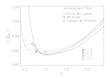
Figure 5: Reduced $\chi^{2}$ as a function of $b_{1}$ for a simulated time series consisting of every fourth image in the isis2 data set and maximal degrees $d=(4,\,2,\,2)$. The average over the twelve non-reference images in the series is denoted by $\langle\chi^{2}_{\mathrm{red}}\rangle$. Curves resulting from Tripp difference imaging runs with four different $\beta$ factors as well and broadening parameters $b=(0.7,\,2.0,\,4.0)$ (AL98), $b=(0.78,\,1.35,\,2.34)$ (W00), and $b=(1.0,\,3.0,\,9.0)$ (GR02) are plotted.

In order to assess the parameter dependence of difference imaging quality in a more realistic (and easily reproducible) form, we utilised a series of 50 simulated crowded field observations contained within the Isis package as test images. These data, hereafter referred to as the isis2 set, show a nearly linear decrease in seeing with index spanning a range from $s\!=\!1.8$ px to $s\!=\!3.2$ px. We took the first image as the reference and every fourth of the further ones as data images. Averaging $\chi^{2}_{\mathrm{red}}$ over the subseries of the latter twelve images, the difference imaging quality for different choices of $b_{1}$ and $\beta$ are presented in fig. 5.

The $\chi^{2}_{\mathrm{red}}(b_{1})$ curves show little variation with the tested $\beta$ except for $b_{1}\!<\!0.8$ px, where there is a steep growth in $\chi^{2}_{\mathrm{red}}$ for $\beta\!=\!1.5$ and, to a lesser extent, for $\beta\!=\!2.0$ as all three broadenings get small relative to the PSF difference. With an optimal value around $b_{1}\!\approx\!1.0$ px, parameters in the interval $0.7~{}\text{px}\leq b_{1}\leq 1.6~{}\text{px}$ yield similarly good results. For the higher three values of $\beta$ a secondary minimum at a smaller $b_{1}$ exists.

Overplotted in fig. 5 are results from Tripp using $d\!=\!(4,\,2,\,2)$ with broadenings taken from the literature: $b\!=\!(0.7,\,2.0,\,4.0)$ (AL98); $b\!=\!(0.78,\,1.35,\,2.34)$ (W00); and $b\!=\!(1.0,\,3.0,\,9.0)$ (GR02). By construction, the latter falls on the $\beta\!=\!3.0$ curve while W00 employs a geometric spacing of $\beta\!\approx\!\sqrt{3}$. The AL98 parameters do not follow a multiplicative relation, but the corresponding $\chi^{2}_{\mathrm{red}}$ value is very close to the ones for those $\beta$ yielding a comparable vector. All of these models come close to the minimum found in our simulations with AL98’s $b_{1}\!=\!0.7$ px marking the lower limit for advisable $b_{1}$.

With a wider $\chi^{2}_{\mathrm{red}}$ valley and its minimum at $b_{1}^{\mathrm{opt}}\!\approx\!2.5$, the isis2 reductions differ significantly from the lorentz results for a width of the data PSF of $s_{\mathrm{dat}}\!\approx\!3.0$ px which is found in the poorer sampled isis2 images. On the other hand, the agreement to the lorentz20 model at $s_{\mathrm{ref}}\!=\!2.0$ px and $\beta\!=\!2.0$ is fairly good (see fig. 4) . This can be explained by the fact that, in current implementations of difference imaging, one set of parameters is chosen for reducing the whole time series comprising images obtained under varying observational circumstances or even collected from several telescopes (as in collaborative microlensing surveys). Given that situation, the averaging selects for the $(b_{g})$ equalising the subtraction residuals over the full observed PSF range.

A closer inspection of the data shows that the overall course of the averaged $\chi^{2}_{\mathrm{red}}$ is determined by the images with best seeing next to the reference image. Their reduction requires slim convolution kernels and thus small $b_{1}$. In order to obtain the best possible lightcurve, a low $\chi^{2}_{\mathrm{red}}$ is especially desirable for images of high quality. This means applying a small $b_{1}$ to the whole data set. Small values of $b_{1}\!\approx\!1.0$ px may not be optimal for wide data PSF relative to the reference, but the loss in terms of $\chi^{2}_{\mathrm{red}}$ compared to the minimum is not large. Therefore, the $(b_{g})$ can be determined by optimising them for the most sensitive data image of best seeing. As a positive side effect, the success of a certain set of $(b_{g})$ can be deduced from a test run on only two images: the reference image and a further good seeing exposure.

4.3 Crowded field tests using lorentz20 data

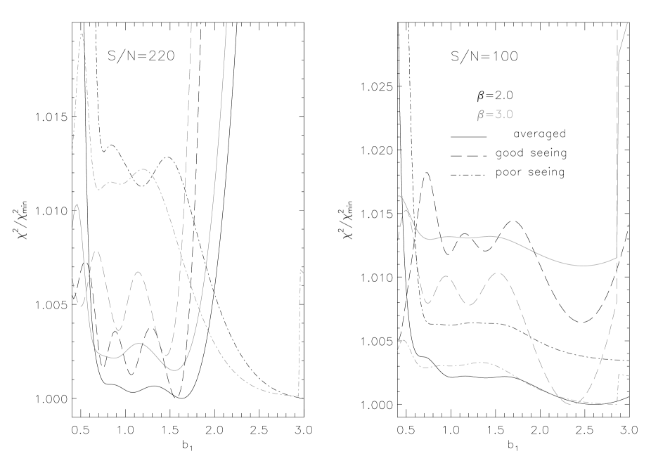
Figure 6: Reduced $\chi^{2}$ as a function of $S/N$ and minimum kernel width $b_{1}$ for a simulated time series of highly blended lorentz20 PSF’s. Shown are $\chi^{2}_{\mathrm{red}}$ averaged over twelve images with linearly increasing PSF widths (solid curves) as well as for the best (long dashes) and worst (dash-dot) seeing data images. Note that, with decreasing $S/N$, the differences between reductions of good and poor sampling images are also reduced. Adding further noise increasingly flattens out the $\chi^{2}_{\mathrm{red}}(b_{1})$ curves.

Divergent dependences on $b_{1}$ for isis2 and lorentz20 data may partly be caused by the obvious differences between lorentz20 and isis2 profiles: isis2 PSFs are of purely Gaussian shape and are highly blended, while the unblended PSF of our test images have extended Lorentzian wings, cut off by an Gaussian envelope.

We investigated the relative importance of these effects in reductions of a simulated time series of images featuring lorentz20 PSFs at about the same level of crowding as in isis2. Three series of $1\!+\!12$ images at different $S/N$ ratios were created using $s_{\mathrm{dat}}\!=\!1.8$ px in the reference images and an increment of $+0.15$ px with each higher index in a series. Thus, roughly the same seeing range as in isis2 is covered. The average $S/N$ integrated over an aperture centered on a relatively isolated star was set at 220 in the highest quality case and reduced to 100 and 30 for the other ones.

Figure 6 shows how $\chi^{2}_{\mathrm{red}}$ depends on $b_{1}$ for the highest and lowest seeing images out of the twelve data images and the averages over the whole series for the $S/N\!=\!220$ and $S/N\!=\!100$ cases. Values of $\chi^{2}_{\mathrm{red}}$ were normalised to the minimum for the specific $S/N$ and sample subset to be able to present the results for different grades of seeing in the same plot. The $S/N\!=\!30$ curves resemble their counterparts of intermediate quality with features smoothed out by the larger random component.

In the high $S/N$ data set, the $\chi^{2}_{\mathrm{red}}$ averaged over the complete sample follows the best seeing data image curve and with $0.7~{}\text{px}\!\leq\!b_{1}\leq\!1.8~{}\text{px}$ displays a similar interval of nearly optimal minimum kernel widths as their $\beta\!=\!2.0$ and $\beta\!=\!3.0$ counterparts from the isis2 series (fig. 5). The shape of the curves $\chi^{2}_{\mathrm{red}}(b_{1})$ for the best and worst seeing images reproduces quite nicely the results found at both $\beta$ for isolated lorentz20 peaks of similar reference and data sampling. In particular, for the best seeing results at $\beta\!=\!2.0$, the positions of the minima agree quite well with the ones for the isolated $s_{\mathrm{dat}}\!=\!2.0$ px and $s_{\mathrm{ref}}\!=\!2.02$ px (upper right panel in fig. 4).

Comparing the heavily blended isis2 and lorentz20 data allows us to estimate the influence of PSF shape on the difference imaging parameters. While pure Gaussian PSFs yield a relatively simple dependence $\chi^{2}_{\mathrm{red}}(b_{1})$, the multiple minima found with lorentz20 data seem related to their more complex PSF structure. Nevertheless, both data sets have in common the range of usable $b_{1}$. Blending itself appears to have only a minor influence on the choice of $b_{1}$.

With increasing level of noise, the optimum in $\chi^{2}_{\mathrm{red}}$ for the best seeing data image is found at larger $b_{1}$, while for the poorest seeing image it becomes less pronounced. These tendencies are probably caused by the less clearly defined PSF in noisy images. It is unclear whether differences between the $\chi^{2}$ levels for the same image at different $\beta$ in the right panel of fig. 6 represent an artefact of the simulation.

5 Conclusion and outlook

Table 1: Summary of the recommended settings for OIS external parameters.

	Maximal	Minimum	Kernel spacing
Situation	degrees	kernel width	parameter
	$(d_{g})$	$b_{1}$	$\beta$
		(px)
General	e.g.
Recommen-	$(4,\,2,\,2)$,	$0.7\ldots 1.2$	$1.5\ldots 3.0$
dation	$(2,\,2,\,2,\,2)$
Small seeing	e.g.
differences	$(4,\,2,\,2)$,	$\approx 0.7$	$1.5\ldots 3.0$
to reference	$(2,\,2,\,2,\,2)$
Good	e.g.
overall	$(4,\,2,\,2)$,	$0.7\ldots 1.2$	$\approx 3.0$
seeing	$(2,\,2,\,2,\,2)$
Improved	e.g.
precision	$(6,\,4,\,2)$,	$0.7\ldots 1.2$	$1.5\ldots 3.0$
required	$(4,\,4,\,2,\,2)$

Optimal image subtraction following the AL98 setup requires about $n\!\gtrsim\!20$ parameters for successful subtraction of constant sources (fig. 2). The improvement with increasing number of parameters is marginal; the most efficient choices for $(d_{g})$ are given in sec. 3.3. A larger number $G$ of principal Gaussian should be favoured over maximal degrees $d_{g}\!>\!4$.

The choice of kernel widths mainly depends on the differences in PSF widths between reference and data images, with eq. (12) giving a crude estimate. Given a sampling of the data image $s_{\mathrm{dat}}\!\gtrsim\!1.5$ px, the $\chi^{2}_{\mathrm{red}}$ of the reduction does not depend critically on the $(b_{g})$. Multiplicative spacing of kernel widths proves to be useful, with $1.5\!\leq\beta\leq\!3.0$ nearly equally recommendable. Due to a small range in widths, values of $\beta\!<\!1.5$ should not be used. For small differences between reference and data samples, high values of $\beta$ yield a wider and thus more comfortable interval of low $\chi^{2}_{\mathrm{red}}$.

Difference imaging has, up to now, applied a single set of kernel widths to a whole time series, comprising exposures of different seeing. Parameters should then be chosen to achieve preferentially good reductions for high quality images showing a small sampling difference to the reference. As outlined in sec. 4.2, this demands for minimum kernel widths in the interval $0.7~{}\text{px}<\!b_{1}\!<1.2$ px able to model minute PSF differences. At even smaller $b_{1}$, basis function themselves become undersampled leading to a higher $\chi^{2}_{\mathrm{red}}$. As a guideline for the user of OIS, these results are summarised in table 1. One can, in principle, go on to define customised $(b_{g})$ for individual images or groups of images to further optimise $\chi^{2}_{\mathrm{red}}$.

Efforts towards this direction are likely to be impeded by the difficulty of deriving quantitative results on the effects of the parameters. The deeper reason is that the AL98 basis functions produce elements in the matrix $\mathsf{M}$ and the vector $\mathsf{c}$ from eqs. (6) and (7) typically spanning $>\!5$ decades, independent of the input images. Although Tripp makes use of the advantages of singular value decomposition, small changes in the image data may in some cases lead to significantly different $\chi^{2}_{\mathrm{red}}$ values. This instability coexists with the general features presented above. Because this problem arises from large numbers introduced by the multiplication with polynomials of pixel indices in the ad hoc definitions in (eq. 9), it should be fruitful to look for alternative definitions of basis functions. Orthogonal functions – e.g. the decomposition of the PSF into shapelets (Refregier 2003) – might have the double advantages of minimising the number of parameters needed and simultaneously allowing for a wider class of PSF corrections to be applied by optimal image subtraction. The matching of seeing conditions with its subtleties continues to be a nontrivial problem which solution holds many scientific and numerical insights.