Cosmology with the Planck cluster sample

Abstract

It has been long recognised that, besides being a formidable experiment to observe the primordial CMB anisotropies, Planck will also have the capability to detect galaxy clusters via their SZ imprint. In this paper constraints on cosmological parameters derivable from the Planck cluster candidate sample are examined for the first time as a function of cluster sample selection and purity obtained from realistic simulations of the microwave sky at the Planck observing frequency bands, observation process modelling and a cluster extraction pipeline. In particular, we employ a multi-frequency matched filtering (MFMF) method to recover clusters from mock simulations of Planck observations. Obtainable cosmological constraints under realistic assumptions of priors and knowledge about cluster redshifts are discussed. Just relying on cluster redshift abundances without making use of recovered cluster fluxes, it is shown that from the Planck cluster catalogue cosmological constraints comparable to the ones derived from recent primordial CMB power spectrum measurements can be achieved. For example, for a concordance $\Lambda$CDM model and a redshift binning of $\Delta z=0.1$, the $1\sigma$ uncertainties on the values of $\Omega_{m}$ and $\sigma_{8}$ are $\Delta\Omega_{m}\approx 0.031$ and $\Delta\sigma_{8}\approx 0.014$ respectively. Furthermore, we find that the constraint of the matter density depends strongly on the prior which can be imposed on the Hubble parameter by other observational means.

1 Introduction

The cosmological potential of galaxy cluster surveys via the SZ effect (Sunyaev & Zeldovich (1970); Sunyaev & Zel’dovich (1972) and Sunyaev & Zeldovich (1980); recent reviews: Rephaeli (1995); Birkinshaw (1999) and Carlstrom et al. (2002)) has been advocated by many theoretical papers in recent years (see e.g. Bartlett (2000); Bartlett (2001); Cohn & Kadota (2005); Haiman et al. (2001); Molnar et al. (2004) etc.). Future measurements of the number density and distribution of clusters will have a profound impact on our understanding of the nature of the Universe (see e.g. Bahcall et al. (1999); Böhringer & Schuecker (2003); Voit (2005)). The SZ effect is due to its redshift independence especially valuable for detecting clusters. Apart from SZ dedicated surveys (ACT; AMI; Amiba; APEX-SZ; SPT; SZA) which observe fractions of the sky, the Planck surveyor satellite, which is scheduled for launch in 2008, will provide detailed full-sky maps at nine different observing frequencies, ranging from 30 to 857 GHz. It is thus a particular suitable instrument to detect the thermal SZ effect owing to its distinct frequency dependence.

Recently several authors have investigated the properties of a Planck SZ cluster sample by applying different object detection algorithms to simulated Planck channel observations (see e.g. Aghanim et al. (2005); Diego et al. (2002); Hansen (2004); Herranz et al. (2002); Kay et al. (2001); Pierpaoli et al. (2005); Schäfer et al. (2006); Schaefer & Bartelmann (2006); White (2003)). For example, Diego et al. (2002) developed a Bayesian non-parametric method to detect clusters in Planck data, which combines Planck frequency channels in such a way that the signal of contaminating components is reduced with respect to the cluster SZ one. Clusters are then extracted from the resulting map by employing SExtractor (Bertin & Arnouts (1996)). Herranz et al. (2002) and Schaefer & Bartelmann (2006) implemented matched and scale adaptive filtering (Sanz et al. (2001)) techniques to recover galaxy clusters and their photometry from Planck multi-frequency observations. While Herranz et al. (2002) work in the Fourier domain and apply the filters to a $12.8\times 12.8$ deg² sky patch, Schaefer & Bartelmann (2006) work in spherical harmonic space and apply the scale adaptive and matched filtering technique to full-sky Planck simulations using the HEALPIX pixelisation scheme (Górski et al. (2005)) to store the data. Also Schulz & White (2003) use a simple matched filtering algorithm to extract clusters from a map resulting from a hypothesised combination of Planck frequency channels. Pierpaoli et al. (2005) discusses a wavelet based method for component separation designed to recover non-Gaussian, spatially localized and sparse signals. A comparison of the selection and contamination of wavelet and matched filtering extraction techniques is given in Vale & White (2006). In Geisbüsch et al. (2005) (hereafter GKH05), we applied a cluster extraction algorithm that combines the Harmonic Space Maximum Entropy Method (HSMEM; see also Stolyarov et al. (2002)) with a Peak Finding Flux Integration method to recover galaxy clusters from realistic full-sky Planck simulations based on the HEALPIX pixelisation scheme. Furthermore, there have been purely theoretical efforts based on the cluster mass function to estimate the power of the Planck cluster catalogue to constrain cosmological model parameters (see e.g. Battye & Weller (2003); Majumdar & Mohr (2004)). Their redshift mass detection limits rely only on simple noise estimates, i.e. the instrumental noise levels, rather than performing realistic simulations and applying cluster extraction algorithms.

Hence, so far there has not been a study that bases its cosmological parameter constraints forecast on selection and contamination estimates derived directly from realistic simulations and SZ cluster extraction algorithms. Therefore, this work attempts for the first time to place constraints on the basis of a realistic Planck cluster detection pipeline. Here we use the popular matched filtering technique to assemble a cluster candidate catalogue, from which by comparison with the cluster input population the selection and contamination of the cluster samples are derived. Based on the cluster catalogue properties (selection and purity), we examine the constraints which can be placed on cosmological parameters, mainly $\Omega_{m}$ and $\sigma_{8}$.

The paper is organised as follows. In section 2 we give a brief definition of the SZ effect. Besides the general composition of (mock) observations at microwave frequencies, the theoretical basics and the formalism of the used cluster extraction method are described in section 3. Section 4 summarises details of our performed mock simulations and discusses their ingredients. The implementation of the cluster detection algorithm is discussed in section 5. Further, in this section properties of the obtained catalogue, mainly its completeness and purity, are investigated. Cosmological constraints obtainable from the detectable cluster abundance based on the efficiency of the extraction method when applied to Planck data (from the Planck cluster sample) under different assumptions of the fiducial cosmology, knowledge about cluster redshifts and the Hubble parameter prior are presented in section 6. Finally, we close our discussion and conclude in section 7.

2 The Sunyaev-Zel’dovich effect in brief

The anisotropy in the microwave band caused by the SZ effect can be separated into two contributions which are distinguished by the origin of energy of the scattering electrons that is responsible for the shift of photon frequency. The total distortion due to the SZ effect is given by

$$\frac{\Delta I_{\nu}}{I_{0}}=g(x)y-h(x)\beta\tau\,,$$ (1)

where $x=h\nu/k_{{\rm B}}T_{0}$ with $T_{0}=2.725\,{\rm K}$ (Mather et al. (1999)) and $I_{0}=2k_{{\rm B}}^{3}T_{0}^{3}/h^{2}c^{2}$. The first term in equation (1) is the so called thermal SZ effect due to the thermal motion of electrons of the intra-cluster gas. The thermal SZ effect has a spectral shape given by

$$g(x)={x^{4}e^{x}\over(e^{x}-1)^{2}}\,\left[x{e^{x}+1\over e^{x}-1}-4\right],$$ (2)

and a frequency independent magnitude, the Comptonization parameter,

$$y={k_{{\rm B}}\sigma_{\rm T}\over m_{e}c^{2}}\,\int\,n_{e}T_{e}\,dl\,.$$ (3)

In hot clusters ($T_{e}>5$keV) the relativistic electrons present slightly modify the spectral shape of the thermal SZ effect (Challinor & Lasenby (1998)). This resulting relativistic correction has not been taken into account in this work, since its effect on the results presented is negligible. The detectability of the effect from thermal (e.g. Pointecouteau et al. (1998)) and non-thermal (e.g. Ensslin & Hansen (2004)) relativistic electrons has been estimated elsewhere. It is still a matter of debate if Planck will be able to detect relativistic SZ contributions. The spectral shape of the second contribution in equation (1), the kinematic SZ effect, is given by

$$h(x)={x^{4}e^{x}\over(e^{x}-1)^{2}},$$ (4)

and its magnitude, $\beta=v_{\rm pec}/c$, depends on the uniform peculiar line-of-sight bulk motion of the cluster’s electron plasma, $v_{\rm pec}$.

$$\tau=\sigma_{T}\,\int\,n_{e}\,dl\,,$$ (5)

is the Thomson optical depth. In the case the cluster can be assumed to be isothermal the Comptonization parameter can be expressed by

$$y=\left({k_{{\rm B}}T_{e}\over m_{e}c^{2}}\right)\tau.$$ (6)

In this paper we concentrate on the thermal SZ effect and treat the kinematic merely as a contaminant to the thermal SZ.

3 Cluster detection method

Before describing the method utilised, a brief schematic overview of the nature of SZ cluster survey observations and known contributing CMB components is given. Based on these considerations an assessment can be made of the requirements that separation techniques have to satisfy. More detailed discussions about which components are of importance to microwave observations at the Planck observing frequencies are presented in section 4.

3.1 Mock observations

The various components contributing to observations at the Planck frequencies have either different physical processes and/or different sources as origin. Their contributions therefore vary with frequency and scale. The SZ effect - the component of interest - as described in the previous section is due to inverse Compton scattering of CMB photons off electrons inside galaxy clusters, which are localised extended objects. In microwave observations the average cluster appears as a source with an extension of the order of a few arcminutes ignoring instrument dependent beam convolution. Several other components of different nature contribute to SZ observations as a background or foreground. Here, we briefly mention the most important ones. First of all, there is the primordial CMB component. According to standard inflationary theories, which are in good agreement with constraints placed by recent observations, this component is a homogeneous random Gaussian field entirely described by its power spectrum. Cumulatively, field point sources contribute in an isotropic manner to SZ observations in the radio and far-infra-red wavelength regime. Furthermore, in the Galactic plane dust, free-free and synchrotron emission from the Milky Way, our Galaxy, also represent within certain wavelength regimes an important source of confusion. The components mentioned so far are all of cosmological or astrophysical nature. The spatial resolution of the observations is limited by the instrument design and the resulting instrumental beam. A component of a different kind, which unavoidably corrupts the observed data is the instrumental noise. Hence, generally, a SZ observation at a single frequency $\nu$ can be modelled by:

$$d_{\nu}({\bf x})=\sum_{i}s_{\nu\,i}({\bf x})+n_{\nu}({\bf x}),$$ (7)

where $s_{\nu\,i}({\bf x})$ is the contribution at position ${\bf x}$ of the $i$th cluster and $n_{\nu}({\bf x})$ gives the cumulative ‘noise’ contribution (including all other components) to the data $d_{\nu}$ at ${\bf x}$. For a single frequency survey $d_{\nu}$ is a scalar field. In the following, $s_{\nu\,i}({\bf x})$ refers to the thermal SZ contribution of the cluster, whereas other SZ components, if present are regarded as noise. Even though point sources are localised objects, in the following their collective contribution is regarded as a single diffuse noise component.

Building on equation (7) a multi-frequency observation is described by:

$${\bf d}({\bf x})=\sum_{i}{\bf s}_{i}({\bf x})+{\bf n}({\bf x}),$$ (8)

where ${\bf d}^{t}=(d_{\nu_{1}},d_{\nu_{2}},...,d_{\nu_{n}})$, ${\bf s}_{i}^{t}=(s_{{\nu_{1}}\,i},s_{{\nu_{2}}\,i},...,s_{{\nu_{n}}\,i})$ and ${\bf n}^{t}=(n_{\nu_{1}},n_{\nu_{2}},...,n_{\nu_{n}})$ are transposed column vectors of the data, the $i$th cluster SZ signal and the noise. Their components are the particular values and contributions respectively at observing frequencies $\nu_{1},\nu_{2},...,\nu_{n}$.

3.2 Matched filtering

This section discusses the matched filtering technique, which utilises spatial as well as spectral information to detect SZ decrements (increments) of galaxy clusters. The literature also refers to it as optimal filter (e.g. Haehnelt & Tegmark (1996)). In which way the matched filter is an optimal one is discussed later in this section. The matched filter is a template cluster extraction method. A common cluster template is, for example, the spherically symmetric $\beta$-profile (see e.g. Cavaliere & Fusco-Femiano (1976)). In this case the observed SZ signal for the $i$th cluster at position ${\bf x}={\bf 0}$ at frequency $\nu_{j}$ is given by:

$$s_{\nu_{j}\,i}({\bf x}) = \int B_{\nu_{j}}({\bf x}-{\bf x}^{\prime})f_{\nu_{j}}A_{\nu_{\rm ref}\,i}\tau({\bf x}^{\prime})d^{2}{\bf x}^{\prime}$$ (9)

$$= \int B_{\nu_{j}}({\bf x}-{\bf x}^{\prime})f_{\nu_{j}}A_{\nu_{\rm ref}\,i}[1+(|{\bf x}^{\prime}|/r_{c\,i})^{2}]^{\frac{1}{2}-\frac{3}{2}\beta}d^{2}{\bf x}^{\prime},$$

where $A_{\nu_{\rm ref}\,i}$ is the amplitude of the $i$th cluster at the reference frequency $\nu_{\rm ref}$, $r_{c\,i}$ determines the spatial cluster scale (cluster core radius), $B_{\nu_{j}}$ is the instrumental beam at frequency $\nu_{j}$ and $f_{\nu_{j}}$ the frequency conversion factor ($f_{\nu_{\rm ref}}=1$). $\tau$ represents the spatial template normalized to unit amplitude.

In constructing the matched filter for a given profile, the noise $n_{\nu_{i}}({\bf x})$ is assumed to be homogeneous with average value $\langle n_{\nu_{i}}({\bf x})\rangle=0$ and cross-power spectrum $P_{{\nu_{i}}{\nu_{j}}}({\bf k})$ defined by:

$$\langle\tilde{n}_{\nu_{i}}({\bf k})\tilde{n}^{*}_{\nu_{j}}({\bf k}^{\prime})\rangle=P_{\nu_{i}\nu_{j}}({\bf k})\,\delta_{\rm D}({\bf k}^{\prime}-{\bf k}),$$ (10)

where $\tilde{n}_{\nu_{i}}({\bf k})$ is the Fourier transform of the noise $\tilde{n}_{\nu_{i}}({\bf x})$, $\tilde{n}^{*}_{\nu_{i}}({\bf k}^{\prime})$ denotes its complex conjungate and $\delta_{\rm D}$ is the Dirac delta function. The homogeneity of the noise ensures that its statistical properties are independent of position. Cosmic backgrounds such as the primordial CMB and point sources, as well as the instrumental noise, meet this requirement of statistical homogeneity. Globally, Galactic components, such as Galactic dust emission, are not homogeneous. However, on the scale of clusters ($\sim$ several arcmin²) homogeneity of these components is a reasonable assumption. Our approach to estimating the background noise cross-power spectrum is discussed in section 4.

Moreover, Galactic and point source contributions are caused by emission processes. Therefore, they (always) cause physically an increment in the observed temperature. This violates the requirement of zero mean and leads to a biasing of the recovered signal amplitude of the $i$th cluster, $A_{\nu_{\rm ref}\,i}$. Assuming a central limit and taking off the zero Fourier mode, the map is modelled in simulations to have a zero mean. This is a fairly safe modelling approach of CMB sky observations since the monopole on the targeted sky patch is usually unobserved by common instrumental designs. The required $\langle n_{\nu_{i}}({\bf x})\rangle=0$ can thus be satisfied. The fact that the zero Fourier mode (monopole) is unobserved has a negligible effect on measured cluster fluxes.

Given the assumptions of zero mean and spatial homogeneity the optimal matched filter is then derived as follows. If the sky is observed at $n_{f}$ frequencies, the most general linear estimator of the amplitude $A_{\nu_{\rm ref}i}({\bf x})$ of cluster $i$ at position ${\bf x}$ is given by:

$$A^{\rm est}_{\nu_{\rm ref}\,i}({\bf x}) = \int\Psi({\bf x}-{\bf x}^{\prime})\cdot{\bf d}({\bf x}^{\prime})\,\mbox{d}^{2}{\bf x}^{\prime}$$ (11)

$$= \sum^{n_{f}}_{j=1}\left(\int\psi_{\nu_{j}}({\bf x}-{\bf x}^{\prime})\,d_{\nu_{j}}({\bf x}^{\prime})\mbox{d}^{2}{\bf x}^{\prime}\right),$$

where $\Psi$ and ${\bf d}$ are column vectors each containing $n_{f}$ components. The components of $\Psi^{t}=(\psi_{\nu_{1}},\psi_{\nu_{2}},...,\psi_{\nu_{n_{f}}})$ are frequency dependent weight functions. $A^{\rm est}_{\nu_{\rm ref}\,i}({\bf x})$ represents the estimate of the cluster SZ signal amplitude. This convolution (equation 11) can be written in Fourier space conveniently as a product:

$$A^{\rm est}_{\nu_{\rm ref}\,i}({\bf x})=\sum^{n_{f}}_{j=1}\left(\int\tilde{d}_{\nu_{j}}({\bf k})\tilde{{\psi}}_{\nu_{j}}({\bf k})e^{-i{\bf k}\cdot{\bf x}}\mbox{d}^{2}{\bf k}\right),$$ (12)

where $\tilde{d}_{\nu_{j}}$ and $\tilde{\Psi}_{\nu_{j}}$ denote the Fourier transform of the data and filter at frequency $\nu_{j}$.

In the case of the matched filter one requires the weight function vector $\Psi$ (the filter) to satisfy the following criteria:

1. The quantity $A^{\rm est}_{\nu_{\rm ref}}$ is an unbiased estimator of the SZ amplitude of the cluster. Thus $\langle A^{\rm est}_{\nu_{\rm ref}}\rangle=A_{\nu_{\rm ref}}$ is required.

2. The variance of the noise of the estimator, $\sigma^{2}$, is minimized by the filter, which ensures that $A^{\rm est}_{\nu_{\rm ref}}$ is an efficient estimator.

The requirement of being an unbiased estimator fixes the normalisation of the filter by:

$$\langle A^{\rm est}_{\nu_{\rm ref}}\rangle-A_{\nu_{\rm ref}}=\int\Psi({\bf x})\cdot{\bf s}({\bf x})\mbox{d}^{2}{\bf x}-A_{\nu_{\rm ref}}=0,$$ (13)

where the brakets $\langle\rangle$ denote an average estimate for a specified spatial cluster template centred at the origin (${\bf x}={\bf 0}$) obtained over many noise realisations. The filter shape is determined by demanding the variance of the estimate,

$$\sigma^{2} = \langle(A^{\rm est}_{\nu_{\rm ref}})^{2}\rangle-\langle A^{\rm est}_{\nu_{\rm ref}}\rangle^{2},$$ (14)

to be minimal. This minimization of $\sigma^{2}$ ensures that the shape of the filter is optimally chosen to be maximally sensitive to modes at which the cluster signal exceeds the noise. The multi-frequency filter satisfying these conditions is given in Fourier space by the matrix equation (see also Haehnelt & Tegmark (1996); Herranz et al. (2002)) :

$$\tilde{\Psi}({\bf k}) = \alpha{\bf P}^{-1}({\bf k})\tilde{{\bf F}}({\bf k}),$$ (15)

$${\alpha} = \left(\int{\tilde{{\bf F}}}^{t}({\bf k})\,{\bf P}^{-1}({\bf k})\,{\tilde{{\bf F}}}({\bf k})\,d^{2}{\bf k}\right)^{-1}$$ (16)

$$= {\sigma}^{2},$$

where $\tilde{{\bf F}}$ is a column vector described by $\tilde{{\bf F}}^{t}=(f_{\nu_{1}}\tilde{B}_{\nu_{1}}\tilde{\tau},f_{\nu_{2}}\tilde{B}_{\nu_{2}}\tilde{\tau},...,f_{\nu_{n}}\tilde{B}_{\nu_{n}}\tilde{\tau})$ and ${\bf P}^{-1}$ is the inverse of the noise cross power spectrum matrix with components $P_{\nu_{i}\nu_{j}}({\bf k})$. Equation 16 gives the so-called multi-frequency matched filter (MFMF), which is an extension of the single-frequency matched filter (SFMF) derived in Haehnelt & Tegmark (1996).

4 Microwave sky simulations

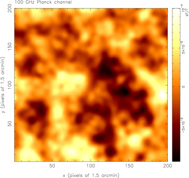
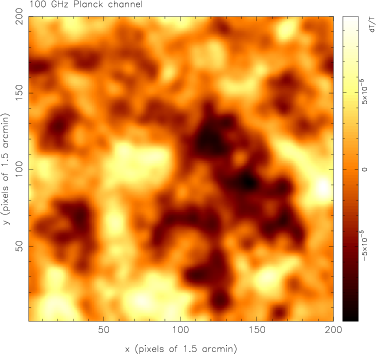
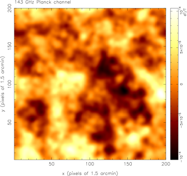
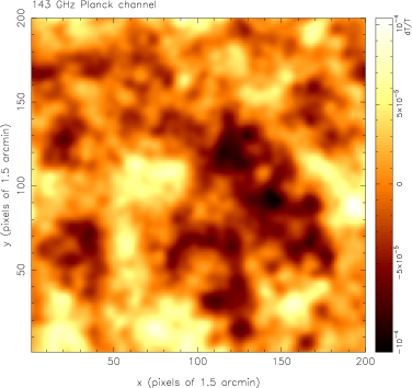
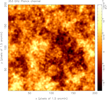
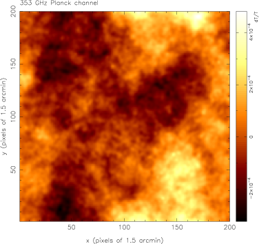
Figure 1: $5\times 5$ deg² realisations of Planck observations at the three observing frequencies of the satellite which are most important for cluster detection via the thermal SZ effect. The upper panels show the observed patches at 100 GHz, the mid panels show the observed patches at 143 GHz and the bottom panels show the observed patches at 353 GHz. The left column shows a patch lying outside the Galactic plane and the right column a patch within the Galactic plane. The same pixelisation scheme and primordial CMB realisation have been adopted for each channel map.

In succeeding sections, extraction algorithms are applied to simulated Planck observations of $5\times 5$deg² sky patches. In particular, data is simulated for the Planck High Frequency Instrument (HFI) channels at 100 GHz, 143 GHz, 217 GHz, 353 GHz, 545 GHz and 857 GHz. Due to their resolution and/or the ratio of the SZ signal in comparison to amplitudes of other fore-/backgrounds within the channel bandwidths, three of these HFI frequency channels - namely the 100 GHz, 143 GHz and 353 GHz channel - are the most useful ones of Planck for galaxy cluster detection via the SZ effect. Simulated sample patches outside and within the Galactic plane observed at the frequencies of these three channels are shown in Figure 1 to give an impression of the expected quality of the Planck mission data. For the purpose of estimating the performance of the extraction techniques when applied to Planck data, patches residing within the Galactic plane and outside of it have been simulated in the right proportion. In the case that observed patches lie within the Galactic plane, the simulations have to include modelling of the Galactic dust, synchrotron and free-free emision besides the primordial CMB, the SZ effects, extragalactic point sources and instrumental effects. Actually, Galactic dust is by far the most dominant Galactic component at the frequencies of interest. Realisations of the Galactic components, the primordial CMB and the SZ effects have been obtained similar to the ones described in GKH05. However, the dust modelling uses this time a two temperature model. Moreover, the anisotropic nature of the Planck instrumental noise on the sky due to the scan pattern of the satellite is taken into account. The extragalactic point source population has been modelled in a different way than previously. Instead of utilising the theoretical model of Toffolatti et al. (1998) as in GKH05, which has been found to match the WMAP point source detections within a factor of two at frequencies below 100 GHz, a phenomenological approach has been taken this time to obtain number counts of the radio and far infra-red/sub-mm point sources at the Planck observing frequencies. Extrapolations of WMAP data (Bennett et al. (2003)) suggest that the contamination due to radio sources is marginal above 100 GHz. While radio point sources dominate below 100 GHz, at the Planck channel frequencies of interest ($\nu\geq 100$ GHz) the confusion caused by dusty luminous infra-red sources is most important. The extragalactic far infra-red/sub-mm (IR/SM) source count modelling performed here is based on the 350 GHz observations of the Submillimetre Common User Bolometer Array (SCUBA; Holland et al. (1999)) mounted on the James Clerk Maxwell Telescope (until 2003). There have been several deep observations made with SCUBA (Smail et al. (1997); Barger et al. (1998); Holland et al. (1998); Hughes et al. (1998); Eales et al. (1999)) from which source counts have been obtained. SCUBA blank field counts of the IR/SM source population on larger fields have been obtained by Scott et al. (2002), Borys et al. (2003) and Scott et al. (2006). From this work one can derive phenomenological fitting formula to the source counts at 350 GHz. The extrapolation of these source counts to lower frequencies ($100\leq\nu\lesssim 300$ GHz), however, involves substantial uncertainties since the spectral behaviour of the sources is not (very) well known and may change significantly from one point source to another. Furthermore, due to a general lack of observations in the frequency regime, knowledge of the emission of extragalactic point sources at intermediate HFI Planck channels is relatively poor and one has to rely on extrapolations based on assumptions about the source spectra. In the (rather unlikely) case of precise knowledge of the spectral behaviour, one could measure the source flux at higher frequencies ($\nu\geq 350$ GHz) at which these sources dominate and subtract off appropriate flux levels at the frequencies of interest. Here, we take a mean spectral index of $\alpha=2.6$ and assume a rms scatter of $\sigma_{\alpha}=0.3$ around this mean for individual galaxies to do the spectral extrapolation. We further assume that IR/SM sources relevant to Planck observations are spatially uncorrelated with clusters detectable by Planck. Given that luminous dusty galaxies are expected to be at high redshifts ($z>1$) this should be a reasonable assumption.

Flat sky patches can be obtained from full sky Planck data by stereographic projection of reasonably sized regions of the sphere onto planes tangential to the sphere at the centres of the patches. Figure 1 shows simulated observations of example patches at three considered Planck channels. Even though the patch shown in the left column lies outside the Galactic plane (low dust region) the identification of galaxy clusters by eye in the map is impossible.

This approach of splitting up the sky into patches is in the case of optimal filtering the preferred one, since background noise levels vary significantly over the full sky. For the matched filter method, it is therefore necessary to have some estimate of the local background noise power spectrum. This knowledge has been assumed to be available (to some realistic degree). For example, it can be gained from the HSMEM separation which has the ability to recover several physical components at ones, each of which is spatially distinct and has a different frequency dependence. However, as a zeroth order estimate of the noise power spectrum one may also take the power spectrum of the sky patch under consideration and then iterate until the extracted cluster number and the power spectrum estimate of the noise converge. Explicitly, this is done by removing in each iteration step the number of clusters detected above a threshold (e.g. above a signal-to-noise threshold of 3$\sigma$) from the map and taking the residual map as the new background noise estimate. If background noise estimates are wrong, the detection significance (signal-to-noise ratio) returned by the method is systematically flawed - hence this is a source of systematic error.

Before applying a MFMF cluster extraction algorithm to the data, one can perform a (pre-)cleaning of the channel maps to reduce the level of certain contaminants and increase the signal-to-noise ratio of the SZ signal. Point sources, for example, can be removed by a Mexican Hat wavelet technique (see e.g. Vielva et al. (2001)). Since the 857 GHz channel is completely and the 545 GHz channel mostly dominated by Galactic dust emission within the plane of our Galaxy after the removal of IR/SM point sources, these channels can be used on their own or in combination to remove the dust emission of the Milky Way at lower frequencies. Furthermore, one might lower the level of primordial CMB contamination by using the 217 GHz channel and performing spatial filtering in spherical harmonic/Fourier space. Herranz et al. (2002) found that if all this cleaning is performed the cluster number count obtained by a MFMF method above a 3$\sigma$ detection threshold is increased by 7 percent and the false detection rate lowered by 12 percent in comparison to the results obtained when the MFMF scheme is applied directly to the ‘raw’ data. At higher signal-to-noise detection thresholds this gain is expected to be even less (in the following a $5\sigma$ detection threshold is used). This suggests that even on its own a MFMF method yields robust and reliable results. Thus such a (pre-)cleaning step has not been included in our analysis pipeline.

5 MFMF cluster extraction

In the following we apply multi-frequency matched filters to the sky observation simulations described above. The filters are constructed according to the instructions given in section 3.2. A cluster candidate catalogue is compiled by using a cluster extraction algorithm based on multi-frequency matched filtering consisting of a number of steps explained in this section.

5.1 Extracting thermal SZ cluster signals

Apart from the initial convolution of the multi-frequency data with the diverse filter kernels to generate a multi-dimensional detection likelihood space, the extraction algorithm consists of several steps which are iteratively repeated until all candidates with detection significances above the required threshold are obtained. The algorithm is similar to the one suggested by Schulz & White (2003).

First, the frequency channel maps are convolved with filters whose spatial scales are gradually varied. The upper and lower limit of the spatial filter scale are determined by the expected range of sizes of detectable clusters on the sky. Besides, performing scale dilation the shape of the cluster template used to construct the filter kernels can also be varied. Since the complexity of several steps of the algorithm scales (linearly) with the diversity of the filter kernels, for a given patch of fixed pixel resolution the computational cost of the algorithm depends strongly on the number of distinct filter kernels applied. The optimal discretisation of the kernels depends on the data at hand. For example, due to the beam sizes of the Planck channels which are rather large in comparison to the average cluster size, one does not expect to gain (much) valuable information about the scales of the unresolved majority of clusters. Thus, a rather coarse filter scaling should be adequate on scales not resolved by the Planck beams. However, as we discuss in section 5.3 otherwise a fine filter scale discretisation is advantageous. In order to construct a detection likelihood space, the convolved multi-frequency channel maps are co-added and normalised to unit variance for each filter kernel as described in section 3.2.

Subsequently, at each iteration the cluster candidate with the highest signal-to-noise ratio is identified in the unit variance normalised ‘detection likelihood space’ spanned (in our case) by the position parameters and the discretized filter scale. A bright cluster has a high detection significance at various filtering scales at (roughly) the same sky position. Its photometric parameters are determined on the basis of the variation of the detection likelihood (peak height in the normalised likelihood space) with filter scale. For the filter scale that is closest to the true scale of the cluster, its signal-to-noise ratio should become maximum. The detection is added to the cluster candidate list and its estimated signal is subtracted from the cube. This removal takes place directly within the detection likelihood space. It is realised by subtracting off an amplitude normalised template at the candidate’s sky position. The template consists of the unit peak (most likely) cluster candidate shape convolved at each scale by the respective filter kernel. Since the number of filter scales is limited, the template can be (pre-)generated and stored for (further) applications of the unaltered algorithm. The amplitude to which the template is finally normalised corresponds to the most likely central cluster candidate SZ distortion in units of the standard deviation of the co-added filter kernel map.

Thereafter, the algorithm is reapplied. The procedure commencing from the step of locating the most significant detection is repeated in a loop on the residual detection likelihood maps until no further detection is found above the chosen signal-to-noise threshold. Thus the extraction algorithm represents an iterative approach similar to a CLEANing procedure (see e.g. Högbom (1974); Clark (1980)). This procedure represents a convenient way to disentangle cluster-cluster confusion as long as the detection of highest significance coincides with the brightest remaining cluster candidate on the patch. This is usually the case. Therefore, by its removal the signal-to-noise ratios of the rest of the candidate detections become unbiased. However, occasionally due to biasing the signal-to-noise ratio of a candidate is overestimated. For example, in the case that filtering at various scales indicates that the projected SZ signal of several clusters might overlap and the single candidate detection significance might be biased due to the overlap or even the detection might be a false one, one has to (re-)assure that the detection significances are to the largest possible extent unbiassed. This can be tested by varying the order of iterative removal of the candidate detections under consideration. It is the candidate whose signal-to-noise ratio varies the least which should be removed first. Such overlaps sometimes occur by chance due to line-of-sight projection over a deep light-cone, as well as in supercluster environments in which clusters are situated close to each other even in redshift space.

Moreover, splitting up the observed patch into seperate regions, in such a way that none of the detections in one region is affected noticeably by one of the other regions and vice versa, speeds up the algorithm slightly by reducing the number of iterations required until all candidate detections above a specified detection threshold are found. The number of iterations reduces from the number of all candidates to the highest number of candidates in one of the seperate regions above the signal to noise threshold. However, the speed up is mostly due to the minimisation of space in which operations have to be performed. It also provides a way to parallelise the extraction algorithm when it is performed on large datasets. The angular clustering of galaxy clusters and the largest scale covered by the set of filter kernels place a lower limit on the patch (region) size. The size has always to be chosen large enough so that all clusters affecting each other are located in the same patch (region).

After completion of the algorithm, a cluster candidate catalogue containing the candidate’s position on the sky, scale, central amplitude, flux, morphological parameters, such as the (asymptotic) slope of the profile, ellipticity and inclination angle, (etc.) is at hand.

5.2 Cluster catalogue properties

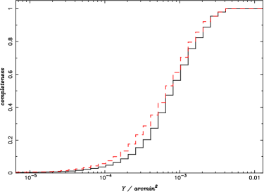
Figure 2: The integrated completeness of the cluster catalogue obtainable from the Planck survey using the MFMF algorithm. Besides matching candidates with single clusters, candidate detections have also been allowed to have several clusters associated with them due to projection along the line-of-sight onto the sky. Single cluster matching is given by the solid line, while multi cluster matching is shown by the dashed line in each case. The integrated completeness is defined as $\mathscr{C}(Y_{\rm cl}\geq Y,z\geq 0)=N_{\rm det}(Y_{\rm cl}\geq Y,z\geq 0)/N_{\rm exp}(Y_{\rm cl}\geq Y,z\geq 0)$, where $N_{\rm det}(Y_{\rm cl}\geq Y,z\geq 0)$ is the recovered number of clusters above a flux $Y$ and $N_{\rm exp}(Y_{\rm cl}\geq Y,z\geq 0)$ is the expected cluster number above $Y$ over the whole sky and redshift range.

After applying the MFMF algorithm to a representive number of sky patches of $5\times 5$ deg² whose noise realisations (instrumental noise levels, Galactic foregrounds) are varied according to the proportion they occupy on the full sky, the properties of the obtained cluster candidate catalogue can be evaluated. For this purpose the candidates have to be associated with real clusters.

5.2.1 Matching up candidates with clusters

Based on the extracted cluster candidate list a matching is performed between candidates and clusters of the input cluster catalogue. Similar as in GKH05, a lower matching flux limit of $Y=3\times 10^{-4}$ is adopted to avoid dubious associations occuring just by chance. This flux threshold corresponds approximately to the analytically derived $3\sigma$ point source sensitivity of Planck (see Haehnelt (1997); Bartelmann (2001)). A candidate is successfully matched up with a real cluster if the distance between their central positions does not exceed a predefined matching length. The association of candidates with clusters is a crucial point in the evaluation of the performance of the extraction method since it affects directly the completeness and contamination estimates. For example, in GKH05 a matching length of just one pixel of $\sim 2$ arcmin was assumed for assigning clusters to candidates recovered from simulated Planck data. Such a conservative matching length leads to firm lower limits of the completeness and purity of the recovered candidate sample since every candidate that is not associated with a cluster due to the small matching length is considered to be a false detection. Henceforth, the extent of the matching length is chosen in a way to account for the fact that cluster candidate positions derived from Planck data are not highly accurate. Positional uncertainties arise mainly due to limited instrumental resolution and noise variations on the resolution scale since cluster core regions even of resolved clusters commonly fit into the Planck instrumental beams. Therefore, we accept a match if the positional deviation (of the pixel centres) does not exceed a matching length of $\sqrt{2}\times{\rm FWHM}$ of the instrumental beam. As the resolution differs with channel, the average FWHM of the beams is taken for constructing the matching distance. Moreover, the pixelisation of the maps is chosen fine enough to ensure that pixelisation effects do not play a (major) role.

In the case that a candidate can be associated with several clusters, it is matched up with the cluster that yields the best flux match. In the reciprocal case of several candidates being matched to one real cluster we proceed in the same way by keeping the best flux match. However, in the following we also consider that multiple clusters are associated with one candidate detection and vice versa. Due to the angular clustering of sources and the fairly large Planck beams, a disentanglement of contributing sources is sometimes impossible and a candidate’s flux estimate can correspond to the sum of several unresolved sources (of even similar flux). In rare cases resolved low redshift clusters are detected as multiple candidates due to noise and background SZ variations on scales smaller than the cluster extent. Then the candidate which fits best the photometry of the real cluster is assigned to it. All the others are conservatively regarded as false detections. Liberally, they are simply disregarded in the case they fall within the matching region of the accepted candidate. As already mentioned above, if a candidate is not matched up with any real cluster above the flux limit, it is regarded as a false detection.

5.2.2 Catalogue completeness and purity

Important measures of the quality of a recovered cluster catalogue are its completeness and purity. These also set benchmarks for the evaluation of how useful the catalogue can be for cosmological purposes. For example, a low completeness results in large uncertainty of the total number of clusters on an observed patch. A catalogue becomes useless if besides a low completeness it possesses as well a low purity. The few positive detections are then diluted by false ones and the catalogue can neither be used to make predictions about the cluster ensemble nor serve as a basis for follow-up observations to learn more about individual objects. If one does not want to rely heavily on observations at other wavelengths (e.g. optical and X-ray cluster observations), which are possibly spoiled themselves, the only way to determine these measures, the completeness and purity, is to perform realistic simulations whose ingredients, such as the underlying cluster sample, are known.

Figure 2 shows the completeness of the catalogue extracted by the MFMF algorithm for candidates detected above a signal-to-noise threshold of 5. Above $Y\sim 10^{-3}$ arcmin² the vast majority of clusters is recovered. At $Y\approx 10^{-3}$ arcmin² the sample is still more than 50 percent complete. Below this flux regime the completeness of the sample falls steeply. The fraction of clusters with a real flux $Y<10^{-3}$ arcmin² that is matched up with a candidate of 5$\sigma$ detection significance is low. As expected, the completeness is increased in the case that multiple clusters are permitted to be assigned to one candidate (see dashed line in Figure 2). At high cluster fluxes this is mainly due to halo clustering in redshift space (supercluster environment). Due to the low surface density of (massive) high flux clusters on the sky, cluster overlap is unlikely to happen just at random (the number density of clusters above the chosen matching flux limit of $Y=3\times 10^{-4}$ arcmin² is well below one cluster per square degree for the assumed cosmological models). Note as well that massive clusters are more strongly clustered than low mass ones. However, the probability of cluster-cluster confusion to occur by chance due to projection along the line-of-sight increases rapidly with decreasing flux. The shown completeness estimate gives an average as expected for a full-sky survey. Note that spatially the completeness varies strongly, depending on the instrumental noise and the Galactic foregrounds.

Further, it turns out that the recovered candidate catalogue is of high purity. The rate of false detections contaminating the sample of candidates with detections of a signal-to-noise ratio of $\geq 5$ is of the order of one percent. Note that due to a limited number of extracted cluster candidates there is always a sample variance error on the estimated purity as well as on the completeness estimate. However, by simulating and analysing an appropriate number of patches which ensures a high number of extracted candidates, the error on the estimates is minimised and a contamination of the candidate sample above $\sim 3$ percent can be excluded at high significance. On the basis of the completeness of this fairly pure recovered cluster sample, cosmological parameter constraints are derived in section 6. In the case the detection threshold is lowered, as expected, the completeness as well as the contamination increase.

5.3 Some remarks

Matched filtering is a template-based object detection approach. To extract the thermal SZ effect, templates empirically derived from fits to observations (e.g. the $\beta$-profile: King (1972) and Cavaliere & Fusco-Femiano (1978)) and/or by hydrostatic theoretical considerations (e.g. Komatsu & Seljak (2002) and Cooray & Sheth (2002)) are utilised. The filter spatial scale is varied by changing the characteristic radius of the cluster template (e.g. the core radius of a $\beta$-profile). Furthermore, one may also parametrise the template shape (e.g. variation of $\beta$ in the case of the $\beta$-profile). The universality of the template is essential to guaranty a photometrically unbiased cluster candidate sample whose signal-to-noise ratio distribution is not systematically skewed. A universal template represents thus an average scalable shape of a cluster SZ imprint in the CMB. Due to different cluster environments and morphologies, the imprints caused by single clusters ‘scatter’ around the average one.

In the case of Planck whose highest resolution of a frequency channel map is 5 arcmin (FWHM), exact knowledge of the cluster SZ template is of less importance than it is the case for high-resolution observations (such as AMI observations), since the convolving instrumental beam erases much of the information on cluster (sub-)structure. Hence, good knowledge of the beam shape is important in the case of Planck. In previous work (Schulz & White (2003)) concerning a matched filter cluster recovery from Planck observations, clusters have been regarded as point sources and the beam shape has been used as template. However, even for ‘low resolution’ Planck data varying template parameters (i.e. building a discretised template library) is advantageous in comparison to a single filter kernel and leads to a larger number of extracted clusters. Nevertheless, the finer the discretisation of the template parameters for constructing matched filtering kernels is, the higher the number of reliably extracted candidates becomes. The computation time needed by the algorithm is raised approximately linearly with filter kernel variety. At some point, however, the increase in consumed computing power outweighs the gain in recovered clusters. Therfore, there is always a trade-off between computational cost and maximising the number of reliably extracted candidates. Our implementation of the MFMF is tuned to be most efficient for Planck data with regard to computational cost and cluster extraction.

The candidate sample (flux) completeness above a chosen flux threshold (see Figure 2) has been derived on the basis of the concordance model and Planck’s instrumental properties. The completeness is no doubt very sensitive to the instrumental design defining the instrumental noise level, resolution and number of frequency channels. Planck’s instrumental properties can be expected to be well known. On the contrary, the noise level due to cosmological contaminants depends like the cluster abundance on the cosmological model of our Universe. While the dependence of the primordial CMB on cosmological parameters is well understood, there is still little known about the cosmological dependence of number counts, auto-/cross-correlations and evolutions of point source populations at Planck’s observing frequencies. Hence, we modelled the point source count empirically on the basis of recent observations. The primordial CMB power spectrum in our simulations has been chosen so that its shape agrees with observational findings from WMAP, VSA and other experiments. Furthermore, we studied the impact of variations of the cluster (surface) number density with cosmology on the completeness. Our testing shows that the completeness is fairly insensitive to such variations at least for reasonable changes of cosmological parameters. This insensitivity can be explained by the in comparison to angular sizes of SZ sources fairly large Planck channel beams which smooth fluctuations in the SZ background. In the case that any significant discrepancies between our assumptions and future observations arise, the algorithms can be rerun on updated simulations to adjust the completeness estimates. Moreover, the absolute number of clusters which will be detectable by Planck depends on several factors. Apart from the cosmology of the Universe which heavily influences cluster detection numbers, also cluster physics plays an important role (see e.g. da Silva et al. (2004)).

6 Expected constraints on cosmology from the Planck SZ survey

It is well known and one of the major motivations of blank field SZ cluster surveys that the cluster abundance and redshift distribution is sensitive to cosmological parameters. On the basis of the ‘blind’ cluster extraction algorithm pursued above and its estimated cluster flux selection (the sample completeness at flux $Y$ and redshift $z$, $\mathscr{C}(Y,z)=N_{\rm det}(Y,z)/N_{\rm exp}(Y,z)$) and purity, in the following the constraints one can obtain from a Planck SZ survey on cosmological parameters are investigated.

6.1 Analysis methodology

The cluster flux dependent selection is found to be approximately universal at redshifts $z\gtrsim 0.1$ for the implemented SZ extraction algorithm. The effect of approximately constant flux sensitivity at redshifts above $z\approx 0.1$ is essentially due to the vast majority of clusters at these redshifts being unresolved. A strong exception to this universality occurs only at very low redshifts. Below $z\lesssim 0.05$ the limiting flux at which the sample has a specific constant completeness increases rapidly to higher fluxes with decreasing redshift. However, since the affected volume is small (low redshift), the number of clusters missed is marginal so that the completeness above a limiting flux at redshift $z$ ($z\gtrsim 0.1$) does not differ from the redshift integrated one as shown in Figure 2 by a large margin. Moreover, all clusters at such low redshifts ($z\lesssim 0.05$) and with SZ fluxes comparable to those in the Planck sample should be (easily) detectable by other observational means. For example, they should have been detected by the ROSAT All Sky Survey (RASS).

For the comparison of the theoretical predictions of the fiducial models with the ones of other models and subsequently for estimating the constraining power of the cluster sample at hand on cosmological parameters, we use a MCMC analysis. Our analysis is based on the Metropolis algorithm (see Metropolis & Ulam (1949)) to sample the (log-)likelihood function over the parameter space. This represents an efficient way of sampling. For the analysis, our basic parameter set consists of four cosmological parameters, $\Omega_{m}$, $\Omega_{\Lambda}$, $\sigma_{8}$ and $h$. Note that we do not assume that the Universe has a flat geometry, as it has been often done in recent works of other authors (see e.g. Battye & Weller (2003) who put their emphasis on constraining the ‘nature’ of dark energy with SZ cluster surveys). Other parameters which generally can be varied as well are kept fixed. For example, the spectral index is fixed to $n_{s}=1$ (Harrison-Zel’dovich spectrum) and the baryon density $\Omega_{b}$ is set to the best fit WMAP value. Furthermore, our presented analysis is restricted to $\Lambda$CDM models ($w=-1$). The inability of cluster surveys on their own to constrain the Hubble parameter, causes us to place in the course of our analysis tight constraints on $h$ obtained by other means, i.e. constraints from the Hubble Space Telescope Key Project (Gaussian prior: $h=0.7\pm 0.08$). Nevertheless, we first examine the effect of a loose uniform $h$ prior on constraints of other parameters. The parameter space spanned by the other cosmological parameters ($\Omega_{m}$, $\Omega_{\Lambda}$ and $\sigma_{8}$) is uniformly sampled in our analysis.

Moreover, in the presented work, running a self-calibration analysis, in which apart from cosmological parameters cluster physics parameters are varied as well, has not been attempted. The normalisation of the mass-Comptonisation parameter (mass-observable) relation of clusters has been assumed to be a priori known and it has been assumed to not evolve with redshift. However, due to the large number of clusters, which is of the order of $10^{3}$ for a detection significance of $5\sigma$ and probable cosmologies of the Universe, such a self-calibration analysis is feasable without abandoning completely meaningful constraints on parameters. Since there is a rather large error on the reconstructed cluster fluxes, only total cluster numbers on the full sky and within chosen redshift bins are used here to derive parameter constraints. Investigating and understanding reconstructed cluster fluxes and deducing a reliable relation between them and real cluster fluxes might allow one to derive even tighter constraints on parameters and eases the grounds for a self-calibration analysis.

On the basis of the cluster flux selection function and the flux to mass conversion, the mean expected cluster number of the fiducial models is compared with theoretical predictions of models by using a Poisson-averaged likelihood in our MCMC analysis (also accounting for the (small) cluster candidate sample impurity which otherwise slightly biases the cosmological parameter constraints). Here, we want to emphasize that the selection functions (depending on cluster flux and redshift) for the performed extraction algorithms are more complex than it has often been assumed in previous analyses of other authors. Most often simple step and symmetric selection functions have been applied in those studies. In the following, the found two dimensional (redshift and flux) selection of the MFMF cluster extraction method is used to derive cosmological parameter constraints. Note further that the choice of the parameterised cluster template can affect the cluster selection and as well bias cluster photometry and thus cosmological constraints. A discrepancy of the presumed template from the average universal one of real clusters causes a reduction in the cluster detection efficiency. Generally, in addition to ignored sources of confusion, the selection function is mostly affected by the choice of the template and its parameterisation. In the case of spatially highly resolved multi-frequency data, a high adaptability of the parameterised template is advantageous. Here, the same cluster template has been used for the SZ simulations and as the detection template. The detection efficiency is thus optimal. In reality, it will be an iterative process to match the parameterised template and its parameter priors to the profiles of real clusters. It would be a good test of the cluster extraction algorithm to apply it to Planck data whose SZ component has been realised by hydrodynamical N-body simulations. However, at present such simulations of cosmic volumes and in quantities as needed to give robust predictions of the cluster selection for the Planck cluster survey are not available.

Furthermore, the conversion used between the real cluster flux and the cluster mass is taken to be universal and assumed to be free of any dispersion. In principle there exists intrinsic scatter in the mass-flux relation due to differences in cluster environments and evolution histories. It is possible to include such an uncertainty in the relation by a convolution of the mass function. However, since hydrodynamical cluster simulations support the assumption that a tight correlation between the cluster mass and flux exists (see e.g. da Silva et al. (2004); Motl et al. (2005)), we neither include a dispersion of the scaling relation in the SZ simulations nor in the following analysis of cosmological parameter constraints. Estimates of the scatter intrinsic to the mass-flux relation obtained from numerical cluster simulations determine it to be of the order of a few percent. In the case one wants to make use of the SZ cluster flux function ($\log S-\log N$) by binning clusters according to their reconstructed fluxes, it is in general not the intrinsic scatter in the mass-flux relation which causes the largest uncertainty of the number of clusters contained in a flux bin. It is rather the scatter of the reconstructed fluxes to the real cluster fluxes that prevents one from finely flux binning the recovered sample. As it can be seen from the flux scatter plots shown in Figure 3 and Figures 9, 10 and 12 of GKH05, which are comparable to the one of the algorithm employed in this work, the uncertainty in the relation of the reconstructed to the real cluster flux exceeds by far for most flux limits except for the highest flux clusters on the sky the intrinsic scatter of the mass-flux relation of individual clusters.

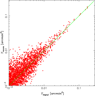
Figure 3: Scatter of the reconstructed cluster fluxes ($Y_{\rm recon}$) versus the real cluster fluxes ($Y_{\rm input}$) of cluster candidates which are matched up with a simulation input cluster by the described matching algorithm. The scatter is shown for fluxes above $Y_{\rm cut}=1\times 10^{-3}$ arcmin².

6.2 Results

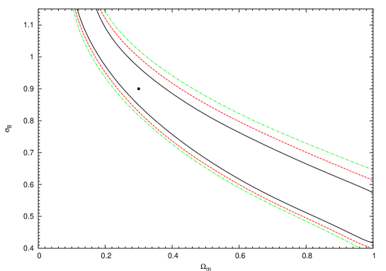
Figure 4: Cosmological parameter constraints on $\Omega_{m}$ and $\sigma_{8}$ from total cluster number counts on the full sky and without cluster redshift information at hand. The 68.3% (black solid line), 95.4% (red dashed line) and 99.7% (green dash-dotted line) confidence levels are shown. The two parameters are degenerate for total number counts. Without prior knowledge by other means only the shape of the degeneracy relation can be constrained. A liberal top-hat prior is placed on the Hubble constant ($0.4\leq h\leq 1$). As fiducial cosmological model the concordance model has been assumed ($\Omega_{m}=0.3$, $\Omega_{\Lambda}=0.7$, $\sigma_{8}=0.9$ and $h=0.7$).

In the following results on parameter constraints are given for several assumptions concerning the restrictions placed on parameters by priors (notably restrictions on the Hubble parameter, $h$) and for different degrees of effort of following-up the cluster sample in the optical for providing cluster redshifts (actually we distinguish between no and complete follow-up). In doing so, we start from weak assumptions and assume an increase in knowledge about the sample redshifts as well as tighten the prior on $h$. These actions lead, as expected, to ever tighter constraints on cosmological parameters obtainable from the cluster sample.

Due to the redshift independence of the SZ effect and due to the resolution of the Planck channels, cluster redshift information cannot be gained from Planck data on its own. In the case of high resolution SZ observations, redshifts can be estimated based on morphological observables (see Diego et al. (2003)). However, the error bars given by the morphological redshift estimation are large. Still such redshift determination might be useful for future SZ surveys, such as the SPT, which will presumably detect thousands of clusters. Obtaining redshifts for such a large number of clusters by follow-up observations at different wavelengths represents currently a major observational effort. Therefore, we first examine the case that no cluster redshift information is available. Figure 4 shows the ‘constraints’ that can be obtained from the total number of SZ detected clusters for $\Omega_{m}$ and $\sigma_{8}$. As expected the two parameters are completely degenerate. One can always find a combination of these two parameters, which mainly govern the mass function, that reproduces the observed total cluster number on the full sky. The particular shape of the degeneracy depends on the survey layout, e.g. the survey depth that can be reached. The degeneracy between $\Omega_{m}$ and $\sigma_{8}$ can be broken somewhat by utilising angular correlation function information (see Mei & Bartlett (2004)). The ‘width’ of the degenerate constraints at a given (fixed) value of $\Omega_{m}$ or $\sigma_{8}$ respectively depends strongly on the range of the $h$ prior. Here we used a uniform prior on $h$ with $0.4\leq h\leq 1$. Another way to break the degeneracy between $\Omega_{m}$ and $\sigma_{8}$ and to constrain $h$ at the same time is to carry out a combined data analysis utilising the Planck cluster sample and the primordial CMB power spectrum (or temperature and polarisation power spectra) obtainable from Planck data.

In our first analysis only the $\Lambda$CDM concordance model ($\Omega_{m}=0.3$, $\Omega_{\Lambda}=0.7$, $\sigma_{8}=0.9$ and $h=0.7$) has been considered as fiducial model. Since the recently published results of the (primordial) cosmic microwave background analysis of the WMAP three year data prefer different parameters than the concordance model, we include apart from the concordance model the best fit WMAP cosmology ($\Omega_{m}=0.27$, $\Omega_{\Lambda}=0.73$, $\sigma_{8}=0.75$ and $h=0.7$) in our examinations and compare the constraints on the parameters of the two models. In particular, the change in $\sigma_{8}$ has an influence on the expected number of clusters recoverable from Planck data.

In order to estimate by how much constraints on cosmological parameters are improved by provided cluster redshift information, we further (optimistically) assume that cluster redshifts are known within some error for the complete Planck cluster sample. This raises questions about the feasability of obtaining cluster redshifts for a major fraction or for the entire sample respectively. The presently least expensive way to measure cluster redshifts is by performing multi-band near-IR and optical imaging observations. First, let us discuss how likely it will be at the time when Planck will have collected its data to have access to optical data for redshift estimations as needed here. With surveys, such as the Sloan Digital Sky Survey (SDSS) and the Two-degree Field Galaxy Redshift Survey (2dFGRS) being already in place and even larger surveys being funded and becoming operational at about the time Planck finishes data collection (e.g. Pan-STARRS, expected to start scanning the sky in 2010), it is not too far-fetched to assume that for a major fraction of the sky optical data of high quality will be available. This assumption of having redshift information available for a large number of Planck clusters is further supported by the fact that the median redshift of the Planck cluster sample of $z\approx 0.2$ matches reasonably well the median redshifts of today’s large scale galaxy surveys (i.e. the galaxy samples of the SDSS have median redshifts of $z\approx 0.104$ (main galaxy sample) and $z\approx 0.35$ (luminous red galaxies) and that of the 2dFGRS is $z\approx 0.11$).

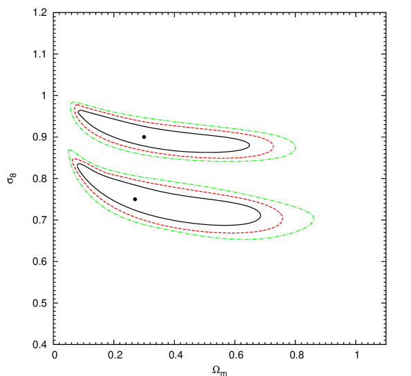
Figure 5: Cosmological parameter constraints on $\Omega_{m}$ and $\sigma_{8}$ from the full sky Planck survey cluster sample.

Furthermore, as the Planck sample contains only (very) massive clusters (commonly $M_{\rm cl}\gtrsim 5\times 10^{14}$ $h^{-1}M_{\odot}$), clusters of the sample will have a high richness (number of member galaxies) and contain many bright galaxies. Further, since the massive clusters of the sample should exhibit a strongly developed red-sequence of galaxies, a deep two-band photometry might be an economical way to gain cluster redshifts of the precision needed for clusters located on the sky remotely from covered optical survey areas. Nevertheless, due to the large uncertainties of the cluster position caused by the rather coarse Planck channel resolutions, pointed follow-up observations of single clusters might be a difficult and cumbersome undertaking. This complicates pointed follow-up observations in optical as well as X-ray wavebands (for a detailed discussion on Planck cluster sample follow-up at different wavelengths and on the expected properties of clusters detectable by Planck in other wavebands see White (2003)). Even in the case of large surveys at optical and/or X-ray wavebands, the recovered positions of Planck detected clusters give only weak constraints for locating associated cluster characteristic features in data collected over wide fields at these wavebands. A similar procedure of matching up Planck detected clusters with detections at other wavebands, as described in section 5.2, has rather to be adopted, after cluster candidates have been located within a matching region at the respective other waveband under consideration. For the case of finding X-ray counterparts, the RASS (Trümper (1991); Voges et al. (1999)) is a good base for providing matches for Planck clusters with redshifts of $z\lesssim 0.3$. The main existing X-ray instruments used these days to detect clusters, XMM-Newton and Chandra, may be not operational anymore at the time when Planck completes its data collection. However, there should be a large overlap between a combined catalogue of cluster detections made by them and the future Planck sample.

Since the Planck cluster sample consists mainly of low redshift massive clusters (the Planck sample is unlikely to contain detections with redshifts $z\gtrsim 1$ for the fiducial cosmological models), already quite shallow multi-band optical surveys covering a wide field (as the ones mentioned above) are well sufficient for cluster redshift determination. Having data of up-coming surveys, such as Pan-STARRS and the Large Synoptic Telescope, available eases the redshift hunt even further. In the following, we use a conservative redshift binning of $\Delta z=0.1$ to group clusters in redshift bins. Ideally one would like to have access to spectroscopic redshifts whose $1\sigma$ precision is commonly better than $\Delta z=0.01$ for an individual galaxy in the redshift range of interest. However, availability of spectroscopic redshifts is likely to be limited. Nevertheless, photomotric redshifts suffice as well for our purposes. For example, photometric redshifts derived from the five SDSS bands are accurate to $\Delta z\sim 0.03$ for an individual galaxy. For a massive cluster hosting several detectable galaxies ($N_{\rm gal}$) the photometrically determined redshift estimate precision increases proportional to $\sqrt{N_{\rm gal}}$. Even for a reasonably deep two-band photometry which uses the 4000 angstrom break of the red cluster sequence galaxies, cluster redshift estimates obtained from colour-magnitude diagrams have uncertainties below $\Delta z\sim 0.05$ for most of the considered redshift range. Therefore, with cluster redshift determination on photometric grounds, redshift bins of $\Delta z=0.1$ are well feasable. Furthermore, our presumed choice of redshift binning is optimal in this respect that it avoids significant cross-correlations between seperate adjacent bins. Covariances between them can therefore be neglected in the analysis.

At first, we derive constraints assuming a very weak prior on the Hubble parameter: $0.02\leq h\leq 5$ (actually this corresponds to $h$ being unconstrained). The resulting obtainable constraints on $\Omega_{m}$ and $\sigma_{8}$ are shown in Figure 5 for the two fiducial cosmologies without requiring the geometry of the Universe to be flat. Since the detected cluster number is statistically relevant, due to the lower number of detected clusters in models with low values of $\sigma_{8}$, as expected, the constraints derived for the WMAP fiducial model are weaker than the ones on the concordance model parameters. While the analysis is able to place reasonable constraints on $\sigma_{8}$ for both fiducial models ($\Delta\sigma_{8}\lesssim 0.08$ at all times), it is barely feasable to gain useful restraining information about the matter density $\Omega_{m}$. However, an Einstein-de Sitter model ($\Omega_{m}=1$) can be excluded at high significance in both cases. Note that on the basis of the performed analysis the two fiducial models exclude each other at several ($\gg 3$) $\sigma$.

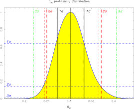
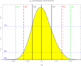
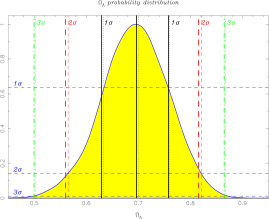
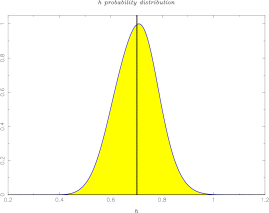
Figure 6: One-dimensional marginalised probability distributions for the cosmological parameters varied in our MCMC analysis. There has been no direct restriction on the curvature $\Omega_{k}=1-\Omega_{m}-\Omega_{\Lambda}$ (no flatness prior). Apart from the Hubble parameter, the remaining parameter sub-space of the other parameters is sampled uniformly. Note that redshift number counts of cluster surveys are most sensitive to $\sigma_{8}$ and in the case of a tight prior on $h$ constrain $\Omega_{m}$. The marginalised distributions are obtained from thinned MCMC sample chains. Thinning ensures that chain samples used for estimating parameter confidence intervals are de-correlated. Chains are thinned in such way that the correlation between consecutive chain steps in the effective thinned chains are below $0.5$ when defining the correlation to be unity at zero step size. All over several million samples are taken to explore the likelihood distribution. We refer the reader to the text for an explanation of the different confidence intervals shown in the panels. Note that, even though a large number of samples has been taken, the error on the 99.7% confidence level of each parameter is rather large due to a still small number of samples located outside this confidence level and thus a resulting large relative sample variance.

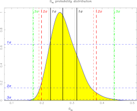
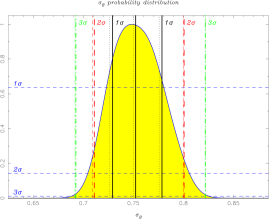
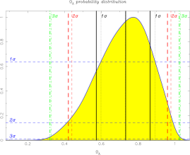
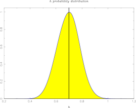
Figure 7: The same as Figure 6 for the WMAP best fit fiducial cosmological parameter model ($\Omega_{m}=0.27$, $\Omega_{\Lambda}=0.73$, $\sigma_{8}=0.75$ and $h=0.7$).

Finally, we place a tight prior on $h$. For the further analysis we constrain the Hubble parameter to $h=0.7\pm 0.08$, as supported by the HST Key Project (Freedman et al. (2001)). Figure 6 and 7 show the marginalised one-dimensional likelihood distributions of the four cosmological parameters, which have been allowed to vary in our analysis, for the two fiducial cosmologies. In addition to the central expectation and fiducial parameter values, various confidence intervals are plotted as well. The dotted central vertical line in each panel indicates the fiducial parameter value. The central thick solid line gives in each case the estimated parameter value gained from the MCMC analysis. Hereby, the shown parameter estimate corresponds to the median of the particular distribution. The other vertical lines give the quantiles of the distributions that are used to quote confidence limits on the parameter constraints. In each case confidence interval lines indicated by different colours and linestyles enclose 68.3% (black solid/dotted), 95.4% (red dashed) and 99.7% (green dot-dashed) confidence regions. Next to the respective confidence interval lines the corresponding confidence level is given in the same colour. The thin lines correspond to quantiles which enclose a particular percentage of the samples of the contributing chains by intersecting the likelihood distribution at the same ‘height’ on both sides of the distribution peak. Thus the area under the graph outside the interval limits adds, for example, (asymmetrically for a non-Gaussian distribution) up in total to 31.7% of the entire area under the graph in the case of the 68.3% confidence region. However, both sides do not have to contribute the same area. The thick lines represent confidence limits obtained from restricting in each case the integrated areas under the graph to be the same on both sides of the distribution peak. This means that for the $1\sigma$ confidence limit interval, 15.85% of the samples of the chains have values below the lower confidence limit and the same percentage of sample values lie above the upper confidence limit. Note that there is no assumption about the distributions being Gaussian. The horizontal dashed blue lines indicate $\exp{(-x^{2}/2)}$ for $x=1$, 2 and 3 respectively. In the case a probability distribution is Gaussian, the intersections of the distribution with the respective line correspond to the $1\sigma$, $2\sigma$ and $3\sigma$ confidence limits respectively. Therefore, if the vertical and horizontal lines do not cross each other at the point at which they intersect the distribution graph, the distribution is non-Gaussian. Moreover, for a Gaussian likelihood distribution the two different ways of placing confidence limits (thin and thick lines) agree. Besides for the Hubble parameter, the marginalised distributions for the most part deviate from a Gaussian one. Even the likelihood distribution of the Hubble parameter which is a priori restricted to a Gaussian is marginally screwed which is caused by degeneracies between $h$ and other variable parameters in the analysis.

The parameter expectation values (median of the particular distribution) gained from the MCMC likelihood analysis together with the 68.3% confidence limits are listed in Tables 1 and 2 for the fiducial models. By comparing the parameter constraints of Tables 1 and 2, it can be seen, parameters are tighter constrained (confidence intervals are smaller) in the case of the concordance model. This is due to the higher number of detectable clusters in the concordance model.

Tight constraints are especially placed on the variance of matter fluctuations on scales of $8h^{-1}$Mpc, $\sigma_{8}$. This is even the case for a less restrictive $h$ prior. Under the made assumptions and set priors (fixed $n_{s}$ and $\Omega_{b}$ and prior on $h$), Planck cluster redshift number counts surpass recent primordial CMB power spectrum measurements in the ability to constrain $\sigma_{8}$. However, loosening the restrictions on the spectral index $n_{s}$ and the baryon density $\Omega_{b}$ weakens constraints on $\sigma_{8}$. On the other hand primordial CMB power spectrum evaluations are well suited to constrain $n_{s}$, $\Omega_{b}$ and $h$. Thus, a combined analysis of the Planck cluster sample and the primordial CMB power spectrum recovered from Planck CMB data is downright recommended. Moreover, combining cluster number counts with investigations of angular (possibly spatial) clustering of the galaxy clusters in the sample and estimates of their gas (baryonic) mass fraction from multi-waveband observations may as well result in a further improvement of constraints which are based on the Planck cluster sample and its follow-up observations.

Furthermore, it is also feasable to derive tight constraints on the matter density parameter $\Omega_{m}$ if a restrictive $h$ prior is set (see Tables 1 and 2). The constraining power of the Planck cluster sample on $\Omega_{m}$ is comparable to the one obtained from the three year WMAP data alone in an analysis with six free parameters assuming the Universe to be flat (see Spergel (2006)). Even the dark energy content $\Omega_{\Lambda}$ and the curvature $\Omega_{k}$ can be constrained. However, they are the ones which of all the parameters in our analysis are least constrained. The 68.3% confidence limits for $\Omega_{\Lambda}$ are given in Tables 1 and 2. By adding $\Omega_{m}$ and $\Omega_{\Lambda}$ of each MCMC chain sample the scatter of the sample curvature values around flatness can be investigated for each fiducial (flat) model since we have not placed priors in our analysis on the geometry of the Universe. Hence, one obtains: $\Omega_{k}=1-\left(0.999^{+0.041}_{-0.041}\right)$ and $\Omega_{k}=1-\left(0.999^{+0.101}_{-0.110}\right)$ respectively.

Parameter	Median ($1\sigma$ constraint)
$\Omega_{m}$	$0.304^{+0.032}_{-0.030}$
$\sigma_{8}$	$0.9^{+0.014}_{-0.013}$
$\Omega_{\Lambda}$	$0.697^{+0.061}_{-0.065}$
$h$	$0.7^{+0.08}_{-0.08}$ (prior)

Table 1: Derived parameter estimates from the MCMC analysis (sample distribution medians) and 68.3% confidence regions with interval limits given by the 15.85% and 84.15% percentiles. The shown constraints are for the concordance $\Lambda$CDM model.

The one-dimensional constraints given in Figures 6 and 7 and in Tables 1 and 2 fail to reveal important information hidden in parameter correlations and degeneracies. In order to display degeneracies between parameters, the two-dimensional joint likelihood distributions for all possible pairs of parameters are shown in Figures 8 and 9 for our fiducial models.

The panels of Figures 8 and 9 display well-known degeneracies between parameters constrained by cluster redshift number counts. For example, the $\Omega_{m}-\sigma_{8}$ degeneracy has been found by many other authors performing an analysis on either simulated (see e.g. Battye & Weller (2003)) or observed data (see e.g. Bahcall & Bode (2003)). Further, the shown correlation between $\Omega_{m}$ and $\Omega_{\Lambda}$ is expected. However, since many authors restrict their analyses to flat models, this degeneracy has been much less studied. The region of acceptable values of $\Omega_{m}$ and $\Omega_{\Lambda}$ ensures that the evolution of the growth factor of linear perturbations is approximately comparable to the one of the fiducial cosmologies in the redshift range of interest. Large deviations in the evolution of linear perturbation growth affect the cluster mass function and thus the expected redshift cluster number count and its slope above a limiting mass significantly. Moreover, the comoving volume element and the limiting mass - both redshift dependent - as well show for the allowed parameter combinations (region of high confidence) over the redshift range covered by the Planck cluster sample only moderate variations from the respective values of the fiducial models. From these two previous degeneracies one can predict the $\Omega_{\Lambda}-\sigma_{8}$ one (see right panel in the second row of Figures 8 and 9). The Hubble parameter $h$ is degenerate to $\Omega_{m}$ and $\Omega_{\Lambda}$. Though, for the found cluster selection it shows little degeneracy with $\sigma_{8}$.

Parameter	Median ($1\sigma$ constraint)
$\Omega_{m}$	$0.269^{+0.047}_{-0.041}$
$\sigma_{8}$	$0.752^{+0.026}_{-0.023}$
$\Omega_{\Lambda}$	$0.736^{+0.132}_{-0.150}$
$h$	$0.7^{+0.08}_{-0.08}$ (prior)

Table 2: The same as Table 1. This time giving the median and $1\sigma$ constraints on the cosmological parameters for an underlying cosmological model with WMAP best-fit parameters.

Note that evidence of the multi-dimensionality of the degeneracies becomes noticeable by comparison of Figure 5 with the left panel in the second row ($\Omega_{m}$-$\sigma_{8}$-plane) of Figure 8 and Figure 9 respectively. The tight prior on $h$ carves out regions around the parameters of each fiducial model to which the constraints are confined. These regions in the two-dimensional parameter space are localised within the two-dimensional constraints plotted in Figure 5. Shifting the mean of the Gaussian prior to a lower value of $h$ shifts the region of high confidence further to the right on the $\Omega_{m}$-axis and marginally downwards on the $\sigma_{8}$-axis. The opposite happens for an increase of the mean value of the Gaussian Hubble parameter prior (while keeping the fiducial parameters unaltered). This illustrates the strong degeneracy between the matter density $\Omega_{m}$ and the Hubble parameter $h$. Therefore, constraining $h$ leads to a strong enhancement of the constraint on the matter density and slightly improves the constraint on $\sigma_{8}$.

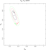
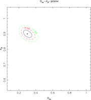
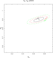
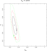
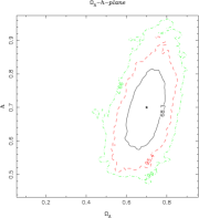
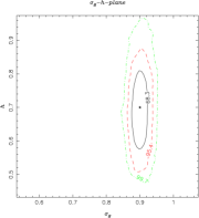
Figure 8: Two-dimensional confidence contours for all pairs of parameters. To obtain the confidence regions we marginalise in each case over the respective other parameters. In each case the contours enclose the 68.3% (black solid line), 95.4% (red dashed line) and the 99.7% (green dot-dashed line) confidence regions. The underlying fiducial model is the concordence $\Lambda$CDM model.

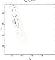
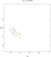
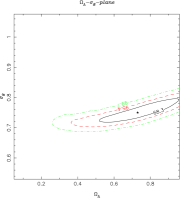
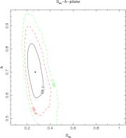
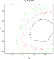
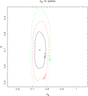
Figure 9: The same as Figure 8 for the WMAP best fit fiducial cosmological parameter model ($\Omega_{m}=0.27$, $\Omega_{\Lambda}=0.73$, $\sigma_{8}=0.75$ and $h=0.7$).

7 Discussion and conclusions

The sky simulation(s) and the modelling of the observing process of the Planck Surveyor satellite presented in this work are of high realism and are based on recent observational constraints and predictions obtained from numerical simulations. Nevertheless, as discussed previously, some uncertainties concerning the component modelling remain. These might even have more than a marginal influence on the results. For example, the modelling of the number counts of IR/SM point sources and their spatial correlation to galaxy clusters is speculative since available observational data are sparse. Apart from a few small patch observations undertaken by SCUBA and MAMBO (see e.g. Greve et al. (2004)), there is little known about the point source population at submillimetre and millimetre wavelengths, resulting in high sample variance and apparently hardly any insight into correlations. Moreover, some channels of the Planck HFI (100 GHz, 150 GHz and 353 GHz) to which IR/SM sources contribute are highly valuable for SZ cluster detections. Therefore, a higher level of point source contamination at these frequencies and/or them being (strongly) spatially correlated with clusters could affect Planck cluster number counts. Furthermore, cluster internal physical processes, such as AGN or SN cluster gas heating, may contribute to the cluster SZ signal in addition to gravitational processes. So far, the mechanisms of these processes occuring at late cluster evolution stages are not well understood. However, the Planck cluster sample should provide an extensive basis for studying such cluster physics.

To the simulated data we have applied a cluster extraction algorithm. The method is a multi-frequency matched filtering technique. It is based on a variational cluster template whose parameters are discretely varied. For this algorithm we optimised the parameter discretisation with respect to algorithm performance and computing cost. Contrary to past analyses which have often restricted the template to be rigid (e.g. Gaussian beam shaped under the assumption that sources are unresolved), the priors on the template parameters have been chosen in such a way that they yield an optimisation of the cluster detection efficiency for the expected quality of the Planck data and cluster physical sizes. The recovered cluster catalogue is then constructed from candidates whose detection significance exceeds $5\sigma$. The built cluster catalogue has been found to be suitable for cosmological considerations under the condition that the survey selection for the data and the adopted algorithm is well understood. For a suitable parameterised selection function, a ‘self-calibration’ is as well feasable due to the large sample size. The extracted catalogue consist of clusters at moderate and intermediate redshifts with cluster masses generally of $M_{\rm cl}\gtrsim 5\times 10^{14}h^{-1}M_{\odot}$. The contamination of the catalogue is found to be fairly low. In general, an expected low sample contamination is a prerequisite in order to be able to use reliably the statistical power of such a large catalogue in addition to a comprehensive sample completeness.

Furthermore, comparing this work with the work presented in GKH05, it is found that the cluster selection is in good agreement with the one found in our previous paper (even though cluster extraction methods differ). In GKH05, due to the strict matching acceptance region of $\sim 2$ arcmins, a certain number of clusters ($\lesssim 10$ per cent above a flux limit of $2\times 10^{-3}$ arcmin²) are not matched up correctly. These missed matches reduce the sample completeness estimate and increase on the other hand the contamination estimate by approximately the same percentage. However, our previous work aimed to give conservative estimates and reliable limits which should be definitely achievable by the Planck cluster sample. On the contrary, overly large matching acceptance regions lead to over-estimates of the completeness and purity above survey flux detection thresholds. This is especially the case for low flux limits and high cluster surface densities, for which overly large acceptance regions increase highly the possibility of finding a match just by chance.

The precision of the photometric cluster parameters of the Planck samples recovered by the applied algorithms is (on the basis of our simulations) expected to be rather poor. This is similar to what we found in GKH05 using a different cluster recovery pipeline. Here, the (relative) dispersion ($\sigma(\log Y)$) of the reconstructed cluster fluxes around their real values is estimated to be approximately 15 percent for the whole sample on average for the recovery by the MFMF method. Though, it is found that the photometric accuracy improves with increasing sample flux threshold. Nevertheless, we have not made use of recovered photometric cluster properties (namely the recovered cluster fluxes) in our parameter analysis. The found large dispersion reduces the usefulness of the recovered cluster fluxes for survey ‘self-calibration’ and cosmological parameter constraints via accurate theoretical mass function predictions, a parameterised mass observable relation and selection function. Likewise, the low photometric quality of the Planck cluster sample affects its cluster physical interpretation in the exact same manner. Therefore, we only touched briefly aspects of late cluster physics in our discussion above. Only global trends, such as the overall (average) normalisation of the $M-Y$ scaling relation, may be grasped by the Planck sample (see GKH05). Constraints on the scaling relation normalisation, however, are expected to be degenerate with cosmological parameters, such as $\sigma_{8}$. One way to improve the understanding of cluster physics is to follow up the sample clusters with observations in the optical and X-ray wavebands. As discussed in section 6, this is a rather cumbersome undertaking. It further has to be pointed out that a template choice differing from the actual universal one biases the photometric parameter estimates (on average) in addition to the large dispersion. However, at the time Planck completes its data collection, several ‘small scale’ SZ experiments will have finished their scientific programmes and obtained results which will give insights into cluster physical aspects, such as cluster profiles, the normalisation of the $M-Y$ relation and its evolution and intrinsic scatter. Therefore, our assumption of available prior information is realistic. These experiments can also be used to follow up the Planck sample in the microwave band enhancing resolution and cluster flux estimations.

Besides optimising cluster extraction and forecasting cluster selection of two powerful algorithms applied to simulated Planck data, we focus on the cosmological prospects which can be accomplished by the Planck cluster sample. This is the first time that based on a realistic selection function derived from astrophysical observation simulations and an implemented data analysis pipeline the cosmological use of the future Planck cluster survey is evaluated. In our MCMC analysis to constrain cosmological parameters, we assume a priori knowledge about the mass observable relation and the cluster selection. As pointed out in the previous paragraph, limits on the $M-Y$ relation normalisation will be obtainable before long by up-comming SZ cluster survey instruments and follow-up of their observations. Insights into the cluster selection function can be achieved by mock observations as presented in this work. However, neglecting or misestimating the magnitude of contaminants leads inevitably to a bias in the expected selection and therefore in the best-fit cosmological parameters obtained from the sample. Note that even in the case of a so-called ‘self-calibration’ analysis some advanced fixings of the parameterised (functional) shape of the selection have to be made. For example, a very common assumption is that the scatter about the mean limiting mass or value of the observable respectively is of Gaussian nature. Apart from mock simulations as performed in this work to estimate the selection function, cross-checks of simulations with data and direct contaminant extraction from data are essential to investigate cluster selection. Reliably pinning down the selection function of the sample will be an iterative process in which results from mock simulations will have to be adjusted to observations in order to make them converge. A number of methods are available to seperate spatially and spectrally diverse components and thus help with estimating the flux selection of clusters. Powerful algorithms for disentangling components are, for example, Independent Component Analysis (ICA) and Maximum Entropy methods (MEM). They may also be applied in order to reduce contamination. However, it is as well possible to estimate the confusion of the cluster fluxes by the MFMF cluster extraction algorithm itself by allowing the level of contamination to vary and including it in the parameter optimisation.

Before summarising the results on constraints, some further challenges the parameter estimation will have to face are outlined. Firstly, uncertainties in cluster physics as well as in cosmological parameters and foregrounds (e.g. IR/SM point sources) suggest that the cluster number contained in the future Planck sample may be uncertain up to a factor of 2-3. The number of recovered clusters evidently controls the statistical ability of the sample to tighten confidence limits on the best-fit parameters. Hence, in section 6 the impact of different the Universe possibly underlying cosmologies on the ability to derive tight cosmological parameter constraints from the respective Planck cluster sample has been investigated. The two different fiducial cosmologies utilised are the concordance $\Lambda$CDM and the best-fit $\Lambda$CDM WMAP model. They differ mainly in their value of $\sigma_{8}$, a parameter which is still fairly little constrained (by today’s standards). Unsurprisingly, the sample with the fewer cluster members (lower value of $\sigma_{8}$) places the weaker constraints on the parameters (about a factor of 1.8 for the $\sigma_{8}$ constraint; see Tables 1 and 2 and Figures 6 and 7). Another concern which is not linked (directly) to the recovery process is the level of accuracy in the theoretical prediction of the cluster mass function. Comparison of large scale numerical (N-body) simulations and halo finding codes estimate the current theoretical uncertainty to be at a level of approximately 10 percent.

Disregarding the theoretical mass function uncertainty, our forecasts suggest that the Planck cluster sample will be able to put tight constraints on cosmological parameters additional to the ones derived from the primordial CMB power spectrum recovered from Planck data. Despite the sample’s rather ‘low’ expected mean redshift, due to the full sky coverage of the survey, cosmological parameter constraints of similar quality as gained from current primordial CMB analyses are realisable. The Planck cluster survey will especially have the capability to tighten constraints on $\sigma_{8}$. The matter variance on scales of 8 $h^{-1}$Mpc is a parameter that can be only ‘weakly’ (in comparison to other parameters) constrained by primordial CMB measurements. All over, current primordial CMB observations on their own are not best suited to place constraints on the shape and normalisation of the matter power spectrum. The large difference of the best-fit $\sigma_{8}$ value of the first and three year WMAP data (which show an approximately $2\sigma$ discrepancy) indicates that the current primordial CMB parameter constraint should possibly not be taken too literally. This notion is strengthened by the fact that several other experiments obtained values discrepant to the WMAP constraint. Large scale structure observations of galaxies and clusters are more suited to place tight constraints on the shape of the matter power spectrum and $\sigma_{8}$. However, most of the large scale structure surveys carried out up to the present day are of such small scale that they are heavily affected by sample variance and ignored systematics may play a role as well. The Planck cluster sample can overcome these problems. Furthermore, degeneracies between parameters, such as $\Omega_{m}$ and $\Omega_{\Lambda}$, obtained from primordial CMB measurements and cluster number counts are different. Therefore performing a combined data analysis helps to narrow down regions of high likelihood in parameter space and to break the parameter degeneracies. Further, we find that while the constraint on $\sigma_{8}$ is only weakly dependent on a prior on the Hubble parameter, constraints on the matter and dark energy density, $\Omega_{m}$ and $\Omega_{\Lambda}$, depend strongly on it. By including a reasonable prior on $h$ in the analysis as given, for example, by the HST Key Project, the confidence intervals of these parameters shrink by up to an order of magnitude. Nevertheless, even without such $h$ prior, the bare existence of a cosmological constant can be confirmed well above the 3$\sigma$ confidence level.

In conclusion, the gain of the Planck cluster catalogue will be twofold. Firstly, it will be a fruitful sample to serve as a base for studying cluster physics (the normalisation, evolution and intrinsic scatter of cluster properties and their scaling relations) in combination with large scale surveys at other wavelengths (RASS, SDSS etc.) and/or follow-up in the microwave band. Secondly, our investigations suggest that the Planck cluster sample (recoverable from future Planck data by algorithms like the one described above) can live up to the high expectations predicted from pure theoretical and analytical estimations by placing meaningful constraints on cosmological parameters. Overall, an all-sky sample of massive clusters with a well understood selection function as achievable by the Planck mission will be of great value for cluster research and cosmology. In a forthcoming paper we will investigate more sophisticated methods than MFMF to examine how their performances improve cluster extraction and constraints on cosmological parameters.

8 Acknowledgements

JG acknowledges an Isaac Newton scholarship from the Cambridge University Isaac Newton Trust and funding from the Cambridge Philosophical Society. JG is grateful to Jim Bartlett and the French Research Ministry for a postdoctoral fellowship. JG thanks the Group PCC/APC formerly at College de France and the head of the Group, Yannick Giraud-Heraud, and the Radio Astronomy Group at the Argelander Institute for Astronomy (University of Bonn) and its head, Frank Bertoldi, for their hospitality. Furthermore, JG acknowledges helpful conversations with Vlad Stolyarov and Mark Ashdown about instrumental properties of the Planck Surveyor satellite.

References

- Aghanim et al. (2005) Aghanim N., Hansen S. H., Lagache G., 2005, AAP, 439, 901
- Bahcall & Bode (2003) Bahcall N. A., Bode P., 2003, ApJL, 588, L1
- Bahcall et al. (1999) Bahcall N. A., Ostriker J. P., Perlmutter S., Steinhardt P. J., 1999, Science, 284, 1481
- Barger et al. (1998) Barger A. J., Cowie L. L., Sanders D. B., Fulton E., Taniguchi Y., Sato Y., Kawara K., Okuda H., 1998, Nature, 394, 248
- Bartelmann (2001) Bartelmann M., 2001, A&A, 370, 754
- Bartlett (2000) Bartlett J. G., 2000, ArXiv Astrophysics e-prints, astro-ph/0001267
- Bartlett (2001) Bartlett J. G., 2001, ASP Conference Series, Tracing cosmic evolution with galaxy clusters, Sesto Pusteria
- Battye & Weller (2003) Battye R. A., Weller J., 2003, PRD, 68, 083506
- Bennett et al. (2003) Bennett C. L., Hill R. S., Hinshaw G., Nolta M. R., Odegard N., Page L., Spergel D. N., Weiland J. L., Wright E. L., Halpern M., Jarosik N., Kogut A., Limon M., Meyer S. S., Tucker G. S., Wollack E., 2003, ApJS, 148, 97
- Bertin & Arnouts (1996) Bertin E., Arnouts S., 1996, AApS, 117, 393
- Birkinshaw (1999) Birkinshaw M., 1999, Physics Reports, 310, 97
- Böhringer & Schuecker (2003) Böhringer H., Schuecker P., 2003, in Holt S. H., Reynolds C. S., eds, AIP Conf. Proc. 666: The Emergence of Cosmic Structure Testing Cosmological Models with Clusters of Galaxies. pp 291–302
- Borys et al. (2003) Borys C., Chapman S., Halpern M., Scott D., 2003, MNRAS, 344, 385
- Carlstrom et al. (2002) Carlstrom J. E., Holder G. P., Reese E. D., 2002, ARA&A, 40, 643
- Cavaliere & Fusco-Femiano (1976) Cavaliere A., Fusco-Femiano R., 1976, A&A, 49, 137
- Cavaliere & Fusco-Femiano (1978) Cavaliere A., Fusco-Femiano R., 1978, A&A, 70, 677
- Challinor & Lasenby (1998) Challinor A., Lasenby A., 1998, ApJ, 499, 1
- Clark (1980) Clark B. G., 1980, A&A, 89, 377
- Cohn & Kadota (2005) Cohn J. D., Kadota K., 2005, ApJ, 632, 1
- Cooray & Sheth (2002) Cooray A., Sheth R., 2002, Physics Reports, 372, 1
- da Silva et al. (2004) da Silva A. C., Kay S. T., Liddle A. R., Thomas P. A., 2004, MNRAS, 348, 1401
- Diego et al. (2003) Diego J. M., Mohr J., Silk J., Bryan G., 2003, MNRAS, 341, 599
- Diego et al. (2002) Diego J. M., Vielva P., Martínez-González E., Silk J., Sanz J. L., 2002, MNRAS, 336, 1351
- Eales et al. (1999) Eales S., Lilly S., Gear W., Dunne L., Bond J. R., Hammer F., Le Fèvre O., Crampton D., 1999, ApJ, 515, 518
- Ensslin & Hansen (2004) Ensslin T. A., Hansen S. H., 2004, ArXiv Astrophysics e-prints
- Freedman et al. (2001) Freedman W. L., Madore B. F., Gibson B. K., Ferrarese L., Kelson D. D., Sakai S., Mould J. R., Kennicutt R. C., Ford H. C., Graham J. A., Huchra J. P., Hughes S. M. G., Illingworth G. D., Macri L. M., Stetson P. B., 2001, ApJ, 553, 47
- Geisbüsch et al. (2005) Geisbüsch J., Kneissl R., Hobson M., 2005, MNRAS, 360, 41
- Górski et al. (2005) Górski K. M., Hivon E., Banday A. J., Wandelt B. D., Hansen F. K., Reinecke M., Bartelmann M., 2005, ApJ, 622, 759
- Greve et al. (2004) Greve T. R., Ivison R. J., Bertoldi F., Stevens J. A., Dunlop J. S., Lutz D., Carilli C. L., 2004, MNRAS, 354, 779
- Haehnelt (1997) Haehnelt M. G., 1997, in Bouchet F. R., Gispert R., Guiderdoni B., Tran Thanh van J., eds, Microwave Background Anistropies Cobras/samba and Measurements of the Sunyaev-Zel Effect. pp 413–+
- Haehnelt & Tegmark (1996) Haehnelt M. G., Tegmark M., 1996, MNRAS, 279, 545
- Haiman et al. (2001) Haiman Z., Mohr J. J., Holder G. P., 2001, ApJ, 553, 545
- Hansen (2004) Hansen S. H., 2004, Lectures given at Varenna summer school, pp 1–12
- Herranz et al. (2002) Herranz D., Sanz J. L., Hobson M. P., Barreiro R. B., Diego J. M., Martínez-González E., Lasenby A. N., 2002, MNRAS, 336, 1057
- Högbom (1974) Högbom J. A., 1974, A&AS, 15, 417
- Holland et al. (1998) Holland W. S., Greaves J. S., Zuckerman B., Webb R. A., McCarthy C., Coulson I. M., Walther D. M., Dent W. R. F., Gear W. K., Robson I., 1998, Nature, 392, 788
- Holland et al. (1999) Holland W. S., Robson E. I., Gear W. K., Cunningham C. R., Lightfoot J. F., Jenness T., Ivison R. J., Stevens J. A., Ade P. A. R., Griffin M. J., Duncan W. D., Murphy J. A., Naylor D. A., 1999, MNRAS, 303, 659
- Hughes et al. (1998) Hughes D. H., Serjeant S., Dunlop J., Rowan-Robinson M., Blain A., Mann R. G., Ivison R., Peacock J., Efstathiou A., Gear W., Oliver S., Lawrence A., Longair M., Goldschmidt P., Jenness T., 1998, Nature, 394, 241
- Kay et al. (2001) Kay S. T., Liddle A. R., Thomas P. A., 2001, MNRAS, 325, 835
- King (1972) King I. R., 1972, ApJL, 174, L123+
- Komatsu & Seljak (2002) Komatsu E., Seljak U., 2002, MNRAS, 336, 1256
- Majumdar & Mohr (2004) Majumdar S., Mohr J. J., 2004, ApJ, 613, 41
- Mather et al. (1999) Mather J. C., Fixsen D. J., Shafer R. A., Mosier C., Wilkinson D. T., 1999, ApJ, 512, 511
- Mei & Bartlett (2004) Mei S., Bartlett J. G., 2004, A&A, 425, 1
- Metropolis & Ulam (1949) Metropolis N. C., Ulam S. M., 1949, J. Amer. Stat. Assoc., 44, 335
- Molnar et al. (2004) Molnar S. M., Haiman Z., Birkinshaw M., Mushotzky R. F., 2004, ApJ, 601, 22
- Motl et al. (2005) Motl P. M., Hallman E. J., Burns J. O., Norman M. L., 2005, ApJL, 623, L63
- Pierpaoli et al. (2005) Pierpaoli E., Anthoine S., Huffenberger K., Daubechies I., 2005, MNRAS, 359, 261
- Pointecouteau et al. (1998) Pointecouteau E., Giard M., Barret D., 1998, A&A, 336, 44
- Rephaeli (1995) Rephaeli Y., 1995, ARA&A, 33, 541
- Sanz et al. (2001) Sanz J. L., Herranz D., Martínez-Gónzalez E., 2001, ApJ, 552, 484
- Schaefer & Bartelmann (2006) Schaefer B. M., Bartelmann M., 2006, ArXiv Astrophysics e-prints, astro-ph/0602406
- Schäfer et al. (2006) Schäfer B. M., Pfrommer C., Hell R. M., Bartelmann M., 2006, MNRAS, 370, 1713
- Schulz & White (2003) Schulz A. E., White M., 2003, ApJ, 586, 723
- Scott et al. (2006) Scott S. E., Dunlop J. S., Serjeant S., 2006, MNRAS, 370, 1057
- Scott et al. (2002) Scott S. E., Fox M. J., Dunlop J. S., Serjeant S., Peacock J. A., Ivison R. J., Oliver S., Mann R. G., Lawrence A., Efstathiou A., Rowan-Robinson M., Hughes D. H., Archibald E. N., Blain A., Longair M., 2002, MNRAS, 331, 817
- Smail et al. (1997) Smail I., Ivison R. J., Blain A. W., 1997, ApJL, 490, L5+
- Spergel (2006) Spergel D. N. e. a., 2006, ArXiv Astrophysics e-prints, 148
- Stolyarov et al. (2002) Stolyarov V., Hobson M. P., Ashdown M. A. J., Lasenby A. N., 2002, MNRAS, 336, 97
- Sunyaev & Zeldovich (1980) Sunyaev R. A., Zeldovich I. B., 1980, ARA&A, 18, 537
- Sunyaev & Zeldovich (1970) Sunyaev R. A., Zeldovich Y. B., 1970, Astrophysics and Space Science, 7, 3
- Sunyaev & Zel’dovich (1972) Sunyaev R. A., Zel’dovich Y. B., 1972, Comm. Astrophys. Space Phys., 4, 173
- Toffolatti et al. (1998) Toffolatti L., Argueso Gomez F., de Zotti G., Mazzei P., Franceschini A., Danese L., Burigana C., 1998, MNRAS, 297, 117
- Trümper (1991) Trümper J. E., 1991, New York Academy Sciences Annals, 647, 141
- Vale & White (2006) Vale C., White M., 2006, New Astronomy, 11, 207
- Vielva et al. (2001) Vielva P., Martínez-González E., Cayón L., Diego J. M., Sanz J. L., Toffolatti L., 2001, MNRAS, 326, 181
- Voges et al. (1999) Voges W., Aschenbach B., Boller T., Bräuninger H., et al. 1999, A&A, 349, 389
- Voit (2005) Voit G. M., 2005, Reviews of Modern Physics, 77, 207
- White (2003) White M., 2003, ApJ, 597, 650