Gravitational Loss-Cone Instability in Stellar Systems
 with Retrograde Orbit Precession

Abstract

We study spherical and disk clusters in a near-Keplerian potential of galactic centers or massive black holes. In such a potential orbit precession is commonly retrograde, i.e. direction of the orbit precession is opposite to the orbital motion. It is assumed that stellar systems consist of nearly radial orbits. We show that if there is a loss cone at low angular momentum (e.g., due to consumption of stars by a black hole), an instability similar to loss-cone instability in plasma may occur. The gravitational loss-cone instability is expected to enhance black hole feeding rates. For spherical systems, the instability is possible for the number of spherical harmonics $l\geq 3$. If there is some amount of counter-rotating stars in flattened systems, they generally exhibit the instability independently of azimuthal number $m$. The results are compared with those obtained recently by Tremaine for distribution functions monotonically increasing with angular momentum.

The analysis is based on simple characteristic equations describing small perturbations in a disk or a sphere of stellar orbits highly elongated in radius. These characteristic equations are derived from the linearized Vlasov equations (combining the collisionless Boltzmann kinetic equation and the Poisson equation), using the action – angle variables. We use two techniques for analyzing the characteristic equations: the first one is based on preliminary finding of neutral modes, and the second one employs a counterpart of the plasma Penrose – Nyquist criterion for disk and spherical gravitational systems.

1 Introduction

Mechanisms of “fuel” supply for galactic nuclear activity usually assume exposure of stars and gas clouds to a non-axisymmetric gravitational potential. The bar mode instability and tidal action from nearby galaxies are most commonly considered to be responsible for formation of the potential (Sulentic & Keel, 1990). We believe, however, that the nuclear activity results from processes in the immediate vicinity of central objects. It is unlikely that large-scale instabilities, such as the global bar mode, can provide for precise targeting of the star or gas flow towards the center.

As an example of local mechanism that can maintain the activity we consider an instability in the stellar environment of the galactic center. This instability has a well-known prototype in plasma physics: the loss-cone instability in the simplest plasma traps similar to mirror machines (see the pioneer paper by Rosenbluth, Post (1965), and, e.g., Mikhailovsky (1974)), which is due to peculiar anisotropy in the velocity distribution of plasma particles. The anisotropy is caused by departure of particles with sufficiently small velocity component transverse to the symmetry axis of the system. The presence of this “loss cone” produces deformation of the plasma distribution function (DF) in transverse velocities, giving it unstable (beam-like) character.

Similar deformation in the DF in angular momentum takes place in clusters in case of deficiency of stars with low angular momentum due to their absorption by the galactic nucleus, black hole, or to other reasons. Then the deformation can have a “beam-like” character: the DF becomes an increasing function of angular momentum, $\partial f_{0}/\partial L>0$. In this case, provided an additional condition discussed later is met, the deformation can trigger the instability which we shall call the gravitational loss-cone instability.

We have mentioned the principal possibility of the instability in, e.g., Polyachenko & Shukhman (1980), and Fridman & Polyachenko (1984). However, the search of a specific example of the gravitational loss-cone instability has been unsuccessful until one of the authors (Polyachenko, 1991b) found the desired instability in a disk model. The delay and initial difficulty in finding it might be due to the unusual character of this instability, which is directly related to relatively very slow precession motion of stellar orbits. Thus typical frequencies and growth rates here are anomalously small, if measured in, for example, orbital frequencies of stars. Yet it does not mean slowness in absolute units taking into account swift growth of all typical frequencies when going from the galactic periphery to its center.

Tremaine (2005) have studied the secular instability, which is identical to the gravitational loss-cone instability. He examined the disk and sphere models of a low-mass stellar system surrounding a massive central object. In such “near-Keplerian” systems, the gravitational force is dominated by a central point mass. For the disk models with arbitrary orbits, Tremaine has found unstable solutions. Note that for disks of nearly radial orbits the instability was proved by Polyachenko (1991b), and we will give here another proof based on the general integral equation for eigen modes (E. Polyachenko, 2005). Stability of spherical systems for arbitrary orbits has also been probed into by Tremaine (2005), who found no evidence of instability for $l\leq 2$ modes. The study for $l\geq 3$ modes in general case is difficult, but it becomes feasible if one restricts consideration to nearly radial orbits. In this paper we show that the loss-cone instability occurs just from $l=3$ (see Sec. 4 and Sec. 5).

For massive black holes in galactic centers, the collisional diffusion and subsequent partial absorption of nearest stars is most often considered as a mechanism providing for nuclear activity (e.g., Lightman, Shapiro (1977); Shapiro, Marchant (1978)). The very existence of the collisionless (collective) mechanism may initiate revision of the dominating viewpoint regarding the nature of the activity. In this paper, however, we present a mere demonstration of the existence of gravitational loss-cone instability in simplest models. An exception is some preliminary estimations of efficiency of the proposed collective mechanism in the Sec. 5.

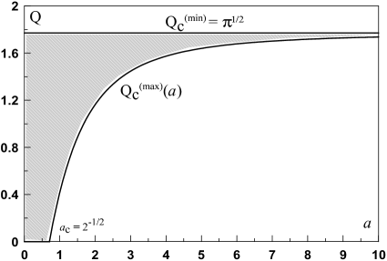
Existence of the above-mentioned additional condition for the instability originates from fundamental distinctions between gravitating and plasma systems. In gravitating systems, particles have only one kind of “charge”, and they attract each other. This fact ultimately leads to the Jeans instability substituting Langmuir oscillations in plasma (e.g. Fridman & Polyachenko, 1984). In systems with nearly radial orbits we are going to study, there is a specific form of the Jeans instability called the radial orbit instability (Polyachenko & Shukhman, 1981; Fridman & Polyachenko, 1984). It develops only in systems with prograde orbit precession (see Fig. 1). Conversely, the gravitational loss-cone instability can occur only when orbit precession is retrograde. This retrograde precession is the additional condition of the instability.

Figure 1: Diagram explaining the physical mechanism of radial orbit instability: a – two typical radial orbits $A_{0}$ and $B_{0}$ in equilibrium state, $A$ and $B$ are their positions in perturbed state from both sides of the perturbed potential minimum (bold dashes) at initial instant of evolution; b – stars at the orbits $A$ (now $A^{\prime}$) and $B$ (now $B^{\prime}$) have gained small angular momentum ($L<0$ at $A^{\prime}$ and $L>0$ at $B^{\prime}$); c – a case of prograde orbit precession (the direction of precession is indicated by arrows): further merging of large axes of orbits takes place, i. e. radial orbit instability develops; d – retrograde precession: return of large axes to the initial equilibrium position, i. e. neutral oscillations. These oscillations can be unstable in the presence of loss cone.

As is well-known, the radial orbit instability is suppressed if the dispersion of orbit precession velocity exceeds some critical value (Polyachenko, 1992). We shall obtain a similar result for the gravitational loss-cone instability (see Sec. 4).

Below we study the gravitational loss-cone instability in two models representing active stellar subsystems with nearly radial orbits. As noted above, the instability in disks was studied earlier in Polyachenko (1991b); Tremaine (2005). Nevertheless, we believe that it merits more detailed consideration here, although the main goal of this paper is to study instability in spherical systems. In Polyachenko (1991b), instability has been determined using the Penrose – Nyquist general criterion (see, e.g., Penrose (1960) or Mikhailovsky (1974)).

In this paper we apply a more illustrative method based on finding neutral modes and subsequent application of the perturbation theory. This allows us to obtain the frequencies and growth rates of perturbations corresponding to small deviations from the neutral modes into the unstable domain. For unstable modes remote from the neutral ones, their complex frequencies are found numerically. At first we shall carry out this instability analysis for a simpler disk model (Sec. 3), then we shall use it for more complicated spherical geometry (Sec. 4).

Another reason for revisiting disks is that a principal characteristic equation in Polyachenko (1991b) was taken ready-made, without derivation. Here we present a detailed derivation of this equation. In addition, we justify the use of a suitable rotating spoke approximation: a spoke consists of stars with fixed energy $E=E_{0}$ and low values of angular momentum $L$. The approximation is then applied to the spherical model.

The paper is organized as follows. The characteristic equations derived in Sec. 3.1 and 4.1 – 4.4 are then applied to studying the gravitational loss-cone instability of disks (Sections 3.2 and 3.3) and spheres (Sections 4.5 – 4.8). In particular, in Sec. 4.8 we obtain general instability criterion for spherical systems analogous to the well-known Penrose – Nyquist criterion for plasma, and establish its correspondence to our neutral-mode approach. The instability of various DF functions is discussed in terms of this criterion. The study is prefaced with an overview of the orbit precession in the axial and centrally-symmetric gravitational fields (Sec. 2). Appendix A is devoted to derivation of a basic integral equation for spherical systems in terms of the action-angle formalism, and in Appendix B we prove the instability criterion theorem.

2 Some remarks on the orbit precession

In low-frequency perturbations of stellar clusters we are interested in, with typical frequencies, $\omega$, of order of the mean precession velocity of near-radial orbits, these latter participate as a whole (in contrast to high-frequency perturbations, for which $\omega$ is of order of orbital frequencies; they depend on individual stars). A detailed justification of these statements (which are fairly obvious) can be found in our papers Polyachenko (1992), E. Polyachenko (2004), Polyachenko & Polyachenko (2004) and in Lynden-Bell (1979). For perturbations of interest, precessing orbits replace individual stars. So a preliminary overview of some useful data on precession becomes very desirable.

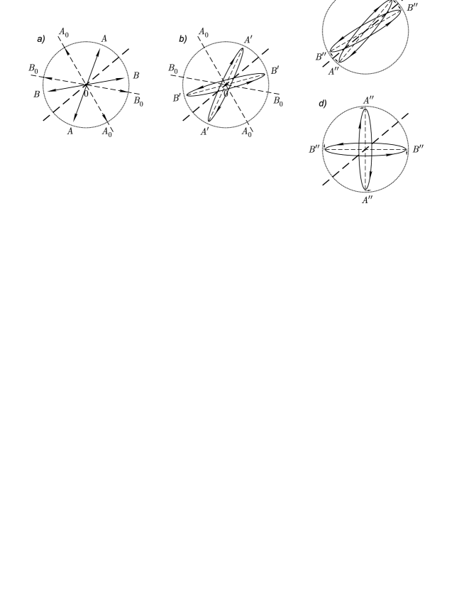
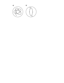
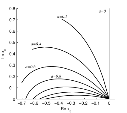
In spherical potentials, star orbits are rosettes that generally are not closed (Landau & Lifshitz, 1976) (see Fig. 2a). It is possible, however, to find a rotating (with angular velocity, $\Omega$) reference frame in which the orbit is a closed oval. Therefore, star movement along the rosette are quick oscillations in a closed oval, which in turn slowly rotates (or precesses) with the rate $\Omega_{\rm pr}=\Omega$ (Fig. 2b). The latter is the orbit precession rate.

Figure 2: Typical stellar orbit in the plane of axially-symmetric disk or in the spherical cluster a – “rosette trajectory” in the inertial system of reference b – closed precessing orbit in a system of reference rotating with angular velocity $\Omega=\Omega_{\rm pr}$.

There are only two potentials (Arnold, 1989) in which any orbits are closed ellipses: (i) for quadratic potential, $\Phi_{0}(r)\propto r^{2}$, the ellipses are symmetric with respect to the center, and (ii) for the point mass potential, $\Phi_{0}(r)=-GM_{c}/r$, in which the orbits (Keplerian ellipses) are asymmetric. The ellipses in these two potentials are resonance orbits, since the ratio of the radial oscillation frequency, $\Omega_{1}$, to that of the azimuthal oscillations, $\Omega_{2}$, is 2:1 for the quadratic potential, and 1:1 for the Keplerian one. As the orbits are closed, the precession rate is zero.

Small deviation from these particular potentials results in a slow precession with the frequency $\Omega_{\rm pr}$ much smaller than the typical frequencies of orbital motion, $\Omega_{1}$ and $\Omega_{2}$. It occurs, for example, in the centers of galaxies. In the absence of a central point mass, the potential is almost quadratic, so the ratio of radial and azimuthal frequencies is close to 2:1. If a point mass is present, this ratio is close to 1:1 in the central region. The deviation from the exact resonance (and thus slow precession) is caused here by gravity of stars around the central point mass.

In smooth potentials, nearly radial orbits, with angular momenta small compared, for example, to the angular momenta of circular orbits with the same energies $E$), are almost resonant for any amplitude of radial oscillations. This statement can be easily proved. Indeed, the azimuthal frequency, $\Omega_{2}$, to radial frequency, $\Omega_{1}$, ratio for a star in the gravitational potential $\Phi(r)$ is, by definition:

$$\frac{\Omega_{2}(E,L)}{\Omega_{1}(E,L)}=\frac{\Delta\varphi}{\pi},$$

where

$$\Delta\varphi=\frac{1}{2}\oint\frac{L}{r^{2}}\frac{dr}{v_{r}(r;E,L)}=\int_{r_{\rm min}}^{r_{\rm max}}\frac{L}{r^{2}}\frac{dr}{\sqrt{2E-2\Phi(r)-{L^{2}}/{r^{2}}\phantom{\big{|}}}}$$ (2.1)

is the rotation angle of the stellar trajectory as its radius changes from $r_{\rm max}$ to $r_{\rm min}$, $E$ is the energy, and $L$ is the modulus of angular momentum.

Now let us calculate the asymptotic behavior of (2.1) for $L\to 0$. To do this, we shall analyze the expression for radial velocity, $v_{r}^{2}=2E-2\Phi(r)-{L^{2}}/{r^{2}}$; its zeros define the turning points.

In the case of a non-singular potential, $\Phi(0)$ is finite, and one may assume $\Phi(0)=0$. Obviously, the left turning point is $r_{\rm min}\approx{L}/{\sqrt{2E}}$. Since at low $L$ the value of $r_{\rm min}$ is small, the main contribution to the integral comes from a region near the lower limit. So we have

$$\int_{r_{\rm min}}^{r_{\rm max}}\frac{L}{r^{2}}\frac{dr}{\sqrt{2E-2\Phi(r)-{L^{2}}/{r^{2}}\phantom{\big{|}}}}\approx\int_{r_{\rm min}}^{\infty}\frac{L}{r}\frac{dr}{\sqrt{2Er^{2}-L^{2}\phantom{\big{|}}}}.$$

Substituting ${(\sqrt{2E}}/{L})\,r=x,$ we obtain

$$\int_{r_{\rm min}}^{\infty}\frac{L}{r}\frac{dr}{\sqrt{2Er^{2}-L^{2}\phantom{\big{|}}}}=\int_{1}^{\infty}\frac{dx}{x\sqrt{x^{2}-1\phantom{\big{|}}}}\$$

and finally $\Delta\varphi=\pi/2.$ Thus, $2\Delta\varphi=\pi$, and the orbit is a straight line which passes (almost) through the center. The absolute value of the ratio $\Omega_{2}/\Omega_{1}$ is 1:2.

Since for the Keplerian potential this ratio is 1:1, the question arises: Is there a continuous transition from the non-singular case, where the ratio is 1:2, to the Keplerian case? If such a transition exists, i.e. if the angle $\Delta\varphi$ can vary smoothly from $\pi/2$ to $\pi$, a full stellar trajectory cannot be a straight line: a radial direction from the apogee to the perigee should change as a star goes from the perigee to the apogee. The angle of rotation is $\pi<2\,\Delta\varphi<2\pi$, and the trajectory looks like spokes of a bicycle wheel. The number of spokes is finite if $\Delta\varphi/\pi$ is rational, otherwise the spokes will fill up a circle.

Now let us consider, for the neighborhood of the center,

$$\Phi(r)=-\frac{\alpha}{r^{s}},\ \ 0<s<2.$$ (2.2)

The family of potentials (2.2) includes both the non-singular potential, corresponding to $s=0$, and the Kelperian potential corresponding to $s=1$. Near the center, the absolute value of the radial velocity is

$$\sqrt{2E-2\Phi(r)-{L^{2}}/{r^{2}}\phantom{\big{|}}}\approx\sqrt{{2\alpha}{r^{-s}}-{L^{2}}/{r^{2}}\phantom{\big{|}}},$$

and thus $r_{\rm min}=\left({L}/{2\alpha}\right)^{1/(2-s)}$. As before, the main contribution to the integral comes from the lower limit, so

$$\int_{r_{\rm min}}^{r_{\rm max}}\frac{L}{r^{2}}\frac{dr}{\sqrt{2E-2\Phi(r)-{L^{2}}/{r^{2}}\phantom{\big{|}}}}\approx\int_{r_{\rm min}}^{\infty}\frac{L}{r}\frac{dr}{\sqrt{2\alpha\,r^{2-s}-L^{2}\phantom{\big{|}}}}.$$

Substitution $\bigl{(}{2\alpha}/{L^{2}}\bigr{)}\,r^{2-s}=x^{2}$ gives $\Delta\varphi={\pi}/{(2-s)}$, which leads to the frequency ratio

$${\Omega_{2}}/{\Omega_{1}}={1}/{(2-s)}.$$ (2.3)

The relation (2.3) connects the non-singular and Keplerian potentials. We would like to stress again that in this case the stellar trajectory has a sharp turn almost in the center.

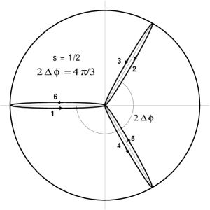
Fig. 3 shows a schematic trajectory in the potential $\Phi(r)\sim-r^{-1/2}$ ($s=1/2)$. One can see the sharp turn of the orbit with the rotation angle $2\Delta\varphi=2\pi/(2-s)=4\pi/3=240^{\circ}$. Numbers $1,\ldots,6$ trace a star in the trajectory. The star moves counter-clockwise, in accordance with the positive sign of the angular momentum, $L>0$. The trajectory is closed since $1/(2-s)$ is a rational number (2/3).

Figure 3: Trajectory of a star with a small angular positive momentum $L$. Parameter $s=0.5$

Further we focus our attention on spherical systems with near-radial orbits in two special gravitational potentials: 1) for a singular near-Keplerian potential, and 2) for an arbitrary non-singular potential. We shall refer to 1:1-orbits in the former case, 2:1-orbits in the latter case. Recall that the most obvious difference between these orbits is revealed in the degenerate case of radial motion: a 1:1-orbit turns into a ray travelling from the center, while a 2:1-orbit turns into a line segment, symmetric to the center.

It turns out (see Introduction) that the gravitational loss-cone instability occurs if the orbit precession is retrograde. Thus it is useful to have expressions for the precession rate, $\Omega_{\rm pr}$, for both types of the orbits at hand.

1:1-orbits.

In the case of a low-mass spherical cluster around the central mass $M_{c}$, one can write

$$(\Omega_{1})^{-1}=\frac{1}{\pi}{\displaystyle{\int\limits_{r_{\rm min}}^{r_{\rm max}}}\dfrac{dr}{\sqrt{2E+{2\,GM_{c}}/{r}-2\Phi_{G}(r)-{L^{2}}/{r^{2}}\phantom{\big{|}}}}}.$$

and

$$\frac{\Omega_{2}}{\Omega_{1}}=\frac{L}{\pi}{\displaystyle{\int\limits_{r_{\rm min}}^{r_{\rm max}}}\dfrac{dr}{r^{2}\,\sqrt{2E+{2GM_{c}}/{r}-2\Phi_{G}(r)-{L^{2}}/{r^{2}}\phantom{\big{|}}}}}\equiv\frac{\Delta\varphi}{\pi},$$

where $\Delta\varphi$ is the rotation angle of a star (cf. (2.1)) in the trajectory between $r_{\rm min}$ and $r_{\rm max}$. If there is no precession, i.e. the contribution of $\Phi_{G}(r)$ to the total potential is negligibly small, the angle would be $\pi$. It is these small deviations of the angle that lead to slow rotation of the elliptical orbit, or precession:

$$\Omega_{\rm pr}=\Omega_{2}-\Omega_{1}=\Omega_{1}\,\left({\Delta\varphi}/{\pi}-1\right).$$ (2.4)

The expression for the precession velocity has obvious sense. After rewriting it in the form

$$\Omega_{\rm pr}=\frac{\Delta\varphi-\pi}{T/2},\ \ \ T=\frac{2\pi}{\Omega_{1}},$$

one can see, that if during one half oscillation, from $r_{\rm min}$ to $r_{\rm max}$ (for the time $T/2$), a star travels an angle exceeding $\pi$, it would imply that the apogee drifts with angular velocity (2.4).

Our goal now is to derive an expression for precession velocity of order ${\cal O}(\Phi_{G})$. Since ${\Delta\varphi}/{\pi}-1={\cal O}(\Phi_{G})$, it is sufficient to retain the ${\cal O}(1)$ order only in calculating the $\Omega_{1}$ factor in (2.4). Then we have

$$\Delta\varphi\approx L\,\frac{\partial}{\partial E}\Bigl{[}(2|E|)^{1/2}\int\limits_{r_{\rm min}}^{r_{\rm max}}\frac{dr}{r^{3}}\,\sqrt{(b-r)(r-a)}-\Big{.}$$

$$-\Big{.}(2|E|)^{-1/2}\int\limits_{r_{\rm min}}^{r_{\rm max}}\frac{\Phi_{G}(r)\,dr}{r\,\sqrt{(b-r)(r-a){\phantom{\big{|}}}}}\Bigr{]}.$$ (2.5)

Here we introduced new variables $a(E,L)=r_{\rm min}(E,L)$ and $b(E,L)=r_{\rm max}(E,L)$, instead of $E$ and $L$, where $a,b={GM_{c}}/{(2|E|)}\,\mp\,\bigl{\{}\bigl{[}{GM_{c}}/(2|E|)\bigr{]}^{2}-{L^{2}}/(2|E|)\bigr{\}}^{1/2}.\ \$ For later purposes, we need some useful relations valid in the Keplerian potential:

$$a\!+\!b=\frac{GM}{|E|},\ a\,b=\frac{L^{2}}{2|E|},\ L=\sqrt{\frac{2GM_{c}\,ab}{a+b}}.$$ (2.6)

One can show that the first item in r.h.s. of (1:1-orbits.) is zero, so one obtains for the precession velocity

$$\Omega_{\rm pr}=-\frac{\Omega(E)}{\pi}\,\frac{\partial}{\partial E}\Bigl{[}{L}\,(2|E|)^{-1/2}\,\int\limits_{a}^{b}\frac{\Phi_{G}(r)\,dr}{r\,\sqrt{(b-r)(r-a){\phantom{\big{|}}}}}\Bigr{]},$$

where $\Omega(E)=\Omega_{1}(E)=\Omega_{2}(E)\approx{(2|E|)^{3/2}}/{GM_{c}}.$ Using (2.6), it is easy to obtain an expression for precession velocity in variables $(a,b)$:

$$\Omega_{\rm pr}=-\dfrac{\Omega}{\pi\,GM_{c}}\,\dfrac{b+a}{b-a}\,\Bigl{(}b^{2}\,\dfrac{\partial}{\partial b}-a^{2}\,\dfrac{\partial}{\partial a}\Bigr{)}\times\\ \times\Bigl{[}\sqrt{a\,b}\int\limits_{a}^{b}\dfrac{\Phi_{G}(r)\,dr}{r\,\sqrt{(b-r)(r-a){\phantom{\big{|}}}}}\Bigr{]},$$ (2.7)

where $\Omega=(GM_{c})^{1/2}\,\bigl{[}{2}/(a+b)\bigr{]}^{3/2}.$ The expression for $\Omega_{\rm pr}$ can be simplified, assuming $a$ to be small (nevertheless, we retain $a$ in the denominator of the argument of the square root):

$$\Omega_{\rm pr}\approx-\dfrac{\Omega(b)}{\pi\,GM_{c}}\,b^{2}\,\dfrac{\partial}{\partial b}\Bigl{[}\sqrt{a\,b}\int\limits_{a}^{b}\dfrac{\Phi_{G}(r)\,dr}{r\,\sqrt{(b-r)(r-a){\phantom{\big{|}}}}}\Bigr{]},$$

where $a^{1/2}={L}/{\sqrt{2GM_{c}\phantom{\big{|}}}}$. It is possible to show that integral $J(a,b)\equiv{\displaystyle\int\limits_{a}^{b}}\dfrac{\Phi_{G}(r)\,dr}{r\,\sqrt{(b-r)(r-a){\phantom{\big{|}}}}}$ may be written as

$$J(a,b)=\int\limits_{a}^{b}\Phi_{G}(r)\,d\Bigl{[}\frac{1}{\sqrt{ab}}\,\arcsin\frac{(b+a)\,r-2ab}{r\,(b-a)}\Bigr{]}.$$

Integrating by parts and then differentiating over $b$ yields:

$$\frac{\partial}{\partial b}\,\left[\sqrt{ab}\,J(a,b)\right]=\int\limits_{a}^{b}\frac{d\Phi_{G}}{dr}\,\frac{1}{b-a}\,\sqrt{\frac{a}{b}}\,\sqrt{\frac{r-a}{b-r}}\,dr\approx\\ \approx\frac{a^{1/2}}{b^{3/2}}\int\limits_{0}^{b}\frac{d\Phi_{G}}{dr}\,\sqrt{\frac{r}{b-r}}\,dr.$$

Finally, we obtain for near-radial orbits:

$$\Omega_{\rm pr}(E,L)=\varpi(E)\,L,$$

$$\varpi(E)=-\frac{2}{\pi GM_{c}\,b}\int\limits_{0}^{b}\frac{d\Phi_{G}}{dr}\,\sqrt{\frac{r}{b-r}}\,dr$$ (2.8)

with $b={GM_{c}}/{|E|}$. From Eq. (1:1-orbits.), it is clear that for such orbits and potentials the precession is always retrograde since $\Phi_{G}^{\prime}(r)=G{\cal M}_{G}(r)/r^{2}>0$, where ${\cal M}_{G}(r)$ is the mass within a sphere of radius $r$. (Moreover, it is easy to show also from (2.7) that for near-Keplerian orbits precession is retrograde even for the case of arbitrary eccentricity (see also Tremaine, 2005)).

Thus, for spherical near-Keplerian systems, the retrograde precession is common. As we will see later, for 2:1-orbits, the situation is vice versa: in real potentials, the precession is prograde, whereas the retrograde precession occurs in systems with exotic density distributions.

2:1-orbits.

There are several different expressions for the precession velocity of near-radial orbits of this type. The expression given in Polyachenko (1992) is somewhat inconvenient for practical use, because it contains a procedure of passage to limit. We shall give a more convenient formula.

For the precession velocity, one has:

$$\Omega_{\rm pr}(E,L)=\Omega_{1}(E,L)\,\Bigl{[}\frac{\Omega_{2}(E,L)}{\Omega_{1}(E,L)}-{\textstyle\frac{1}{2}}\Bigr{]}.$$

The goal is to calculate the derivative of the precession velocity at constant $E$ and $L=0$, i.e. $\bigl{[}{\partial\Omega_{\rm pr}(E,L)}/{\partial L}\bigr{]}_{L=0}$. Taking into account that $\Omega_{1}(E,L)=\Omega(E)+{\cal O}(L^{2})$, one obtains

$$\Omega_{\rm pr}(E,L)\approx\Omega(E)\left({\Delta\varphi}/{\pi}-{\textstyle\frac{1}{2}}\right),$$

where

$$\Delta\varphi=\!\!\!\int\limits_{r_{\rm min}(E,\,L)}^{r_{\rm max}(E,\,L)}\frac{L}{r^{2}}\frac{dr}{\sqrt{2E-2\Phi_{0}(r)-{L^{2}}/{r^{2}}}},$$

is the rotation angle of a star in the trajectory between $r_{\rm min}$ and $r_{\rm max}$, which is equal to $\frac{1}{2}\,\pi$ for any non-singular potential, in the leading order in $L$. The next (linear) term in expansion of $\Delta\varphi$ gives a value of the precession velocity and defines the direction of precession (prograde or retrograde), for a highly elongated orbit, with a small angular momentum. It is clear that if $\Delta\varphi>\pi/2$ (or $2\Delta\varphi>\pi$), the precession direction coincides with the rotation of a star (prograde precession), and vice versa. Thus, the sign of the derivative ${\partial/\partial L}\left(\Delta\varphi-\pi/{2}\right)$ determines the precession direction. Let us denote $\phi(E,L)=\Delta\varphi-{\pi}/{2}$, so that

$$\varpi(E)\equiv\bigl{[}{\partial\Omega_{\rm pr}(E,L)}/{\partial L}\bigr{]}_{L=0}=\frac{\Omega(E)}{\pi}\,\bigl{[}{\partial\phi(E,L)}/{\partial L}\bigr{]}_{L=0}.$$ (2.9)

We have

$$\Delta\varphi=\!\!\!\int\limits_{r_{\rm min}(E,\,L)}^{r_{\rm max}(E,\,L)}\frac{L}{r^{2}}\frac{dr}{\sqrt{2E-2\Phi_{0}(r)-{L^{2}}/{r^{2}}}}=\\ \frac{\partial}{\partial E}\int\limits_{r_{\rm min}(E,\,L)}^{r_{\rm max}(E,\,L)}\frac{L}{r^{2}}\,\,\sqrt{2E-2\Phi_{0}(r)-{L^{2}}/{r^{2}}}\,dr.$$

Integrating by parts yields

$$\Delta\varphi=\frac{\partial}{\partial E}\int\limits_{r_{\rm min}}^{r_{\rm max}}\frac{L^{3}}{r^{4}}\,\,\frac{dr}{\sqrt{2E-2\Phi_{0}(r)-{L^{2}}/{r^{2}}}}-\\ -L\,\frac{\partial}{\partial E}\int\limits_{r_{\rm min}}^{r_{\rm max}}\frac{\Phi_{0}^{\prime}(r)}{r}\,\,\frac{dr}{\sqrt{2E-2\Phi_{0}(r)-{L^{2}}/{r^{2}}}}.$$

One can show that the main contribution to the first integral comes from the lower limit, thus one can extend the integration to infinity. Since, for non-singular potentials, one can neglect $\Phi_{0}(r)\approx\Phi(r_{\rm min})$ (as compared to $E$) in the root argument, we obtain

$$\int\limits_{r_{\rm min}(E,\,L)}^{r_{\rm max}(E,\,L)}\frac{L^{3}}{r^{4}}\,\,\frac{dr}{\sqrt{2E-2\Phi_{0}(r)-{L^{2}}/{r^{2}}}}=\\ =2E\int_{1}^{\infty}\frac{dx}{x^{3}\sqrt{x^{2}-1}}={\textstyle\frac{1}{2}}\,\pi E,$$

so for $\phi(E,L)$ we get:

$$\phi(E,L)\approx-L\,\frac{d}{dE}\int\limits_{0}^{r_{\rm max}(E,\,0)}\frac{\Phi_{0}^{\prime}(r)}{r}\,\,\frac{dr}{\sqrt{2E-2\Phi_{0}(r){\phantom{\big{|}}}}}.$$

Substituting this into (2.9), we find

$$\varpi(E)=-\dfrac{\Omega(E)}{\pi}\,\dfrac{d}{dE}\int\limits_{0}^{r_{\rm max}(E)}\dfrac{\Phi_{0}^{\prime}(r)}{r}\,\,\dfrac{dr}{\sqrt{2E-2\Phi_{0}(r){\phantom{\big{|}}}}}.{\phantom{\Bigg{|}}}$$ (2.10)

There is also an alternative expression, without differentiation with respect to $E$. Omitting details, we give the final expression:

$$\varpi(E) =\dfrac{\Omega(E)}{\pi}\,\Bigl{[}\int\limits_{0}^{r_{\rm max}(E)}\dfrac{dr}{r^{2}}\,\Bigl{(}\dfrac{1}{\sqrt{2E-2\Phi_{0}(r){\phantom{\big{|}}}}}-\dfrac{1}{\sqrt{2E}}\Bigr{)}\Bigr{.}-$$

. $$-\dfrac{1}{r_{\rm max}(E)\,\sqrt{2E}}\Bigr{]}.$$ (2.11)

From the derived expressions it follows, for example, that for the expansion of a potential, $\Phi_{0}(r)=\Phi_{0}(0)+\Omega_{0}^{2}\left(\textstyle\frac{1}{2}\,r^{2}+\beta\,r^{4}+\cdots\right)$, at small $r$, the precession direction is determined by the sign of $\beta$, since $\varpi=-\beta$. Thus, stars with small radial amplitude have retrograde precession if $\beta$ is positive. From Poisson’s equation one immediately has

$$\rho(r)=\frac{1}{4\pi Gr^{2}}\frac{d}{dr}\,r^{2}\frac{d}{dr}\,\Phi_{0}(r)=\frac{3\Omega_{0}^{2}}{4\pi G}\,\Bigl{(}1+\frac{20}{3}\beta r^{2}\Bigr{)},$$

i. e. density increases with radius. Such behavior is unrealistic, and we conclude that the gravitational loss-cone instability is impossible in spherical clusters with non-singular potentials. Note that in disk systems this instability is possible (Polyachenko, 1991b).

3 Gravitational Loss-Cone Instability in Disks

3.1 Derivation of an equation for eigenmode spectra

The simplest relations for describing the instability under study can be obtained in a model with an active stellar subsystem in the form of a disk with nearly-radial orbits. The aim of this Section is to derive characteristic equations for small perturbations in such a model. The derivation involves a series of successive simplifications of the initial linearized Vlasov equations.

Omitting a number of those steps, we take, as the starting point, the following integral equation:

$$\Phi_{l}(E,L)=\frac{G}{2\pi}\int\int\frac{dE^{\prime}\,dL^{\prime}}{\Omega_{1}(E^{\prime},L^{\prime})}\\ \times\sum\limits_{l^{\prime}=-\infty}^{\infty}\frac{\bigl{[}m\,\Omega_{2}(E^{\prime},L^{\prime}){\phantom{\Bigg{|}}}\!\!+l^{\prime}\,\Omega_{1}(E^{\prime},L^{\prime})\bigr{]}\,{\partial F}/{\partial E^{\prime}}+m\,{\partial F}/{\partial L^{\prime}}}{\omega-m\,\Omega_{2}(E^{\prime},L^{\prime})-l^{\prime}\,\Omega_{1}(E^{\prime},L^{\prime}){\phantom{\Bigg{|}}}}\times\\ \times\Pi_{l,\,l^{\prime}}(E,L;E^{\prime}L^{\prime})\,\Phi_{l^{\prime}}(E^{\prime},L^{\prime}).$$ (3.1)

Here $G$ is the gravitational constant, the frequencies $\Omega_{i}=\partial H_{0}/\partial I_{i}$, or more briefly, ${\bf\Omega}({\bf I})=\partial H_{0}/\partial{\bf I}$, $H_{0}({\bf I})$ is the Hamiltonian of a star in unperturbed state, ${\bf I}=(I_{1},I_{2})$ are the actions, $\omega$ is the frequency of a perturbation, $E$ and $L$ are the energy and the angular momentum, respectively, $F=F(E,L)$ is the unperturbed DF, and the Fourier components $\Phi_{l}(E,L)$ and the kernel $\Pi_{l,\,l^{\prime}}(E,L;E^{\prime},L^{\prime})$ are defined as follows:

$$\Phi_{l}(E,L)\!=\!\frac{1}{2\pi}\int_{-\pi}^{\pi}\!\!\!dw_{1}\,\Phi[\,r(E,L;w_{1})]\,\cos[\,lw_{1}\!+\!m\,\chi(E,L;w_{1})],$$

where $\Phi(r)$ is the radial part of the perturbed potential $\Psi(r,\varphi;t)=\Phi(r)\,e^{-i\omega\,t+i\,m\varphi}$, $t$ is the time, $\varphi$ is the polar angle, $m$ is the azimuthal index, $w_{1}$ is the angle conjugate to the radial action $I_{1}$, $l$ is the integer index,

$$\Pi_{l,\,l^{\prime}}(E,L;E^{\prime},L^{\prime})=\int_{-\pi}^{\pi}dw_{1}\cos\,[\,lw_{1}+m\,\chi(E,L;w_{1})]\\ \times\int_{-\pi}^{\pi}\!\!\!dw_{1}^{\prime}\cos\,[\,l^{\prime}w_{1}^{\prime}+m\,\chi(E^{\prime},L^{\prime};w_{1}^{\prime})]\,\\ \times\psi[r(E,L;w_{1}),r^{\prime}(E^{\prime},L^{\prime};w_{1}^{\prime})],\\ \psi(r,r^{\prime})=\int_{0}^{2\pi}d\theta\,\frac{\cos m\theta}{\sqrt{r^{2}+r^{\prime 2}-2rr^{\prime}\cos\theta{\phantom{\big{|}}}}}.$$

The function $\chi$ is defined by

$$\chi(E,L;w_{1})=\Omega_{2}(E,L)\!\!\!\!\!\!\!\!\!\int\limits_{r_{\rm min}(E,\,L)}^{r}\!\!\!\!\!\!\!\frac{dx}{v_{r}(E,L;x)}-\\ -L\!\!\!\!\!\!\!\!\!\int\limits_{r_{\rm min}(E,\,L)}^{r}\!\!\!\!\!\!\!\!\!\frac{dx}{x^{2}v_{r}(E,L;x)}$$

(where $v_{r}$ is the radial velocity of a star), or $\chi(E,L;w_{1})=(\Omega_{2}/\Omega_{1})\,w_{1}-\delta\varphi,$   where

$$\delta\varphi=L\!\!\!\int\limits_{r_{\rm min}(E,\,L)}^{r}\frac{dx}{x^{2}v_{r}(E,L;x)}.$$

For definiteness, we consider systems consisting exclusively of 2:1-orbits in this Section. However, the final form of the desired equation for the case of 1:1-orbits (i.e., for near-Keplerian systems) is practically identical to that for 2:1-orbits. It is evident that slow modes, with angular rates of the order of the typical precession velocity, in the systems with 2:1-orbits are possible only when the azimuthal index $m$ is even. In case of 1:1-orbits the azimuthal number $m$ is arbitrary.

Although the equation (3.1) is an exact linear integral equation that allows one to determine the spectrum of eigenmodes for an arbitrary distribution of stars in the disk, for a stellar system with low angular momenta we are interested in, this equation is inconvenient as the system can include stars with both direct ($L>0$) and inverse ($L<0$) orbital rotation. The point is that the orbital frequency $\Omega_{2}(E,L)$ is discontinuous at $L=0$: $\Omega_{2}(E,L=\pm\,0)={\textstyle\frac{1}{2}}\,{s_{L}}\,\Omega_{1}(E,L=0),\ \ s_{L}\equiv{\rm sign}\,(L)$. So all items in the sum over $\ l^{\prime}$ are also discontinuous at $L^{\prime}=0$. The function $\Phi_{l}(L)$ itself and the kernel of the integral equation $\Pi_{l,l^{\prime}}(L,L^{\prime})$ are discontinuous too. (Hereafter we shall omit the arguments $E$ and $E^{\prime}$, provided this creates no difficulties.) The discontinuity is very inconvenient. In fact it arises from a poor choice of the angle variables in the set of actions – angles, for the problems of interest involving stars with $L<0$ (note that discontinuity is quite inessential in problems with nearly-circular orbits (see, e.g., E. Polyachenko 2005). However, this difficulty is fictitious, and actually the equation can be transformed into a continuous form by means of a proper procedure that involves shifting of indices and transformation of the functions. The procedure is simple but cumbersome, so we give the final form of the integral equation without going into detail:

$$\phi_{n}(E,L)=\frac{G}{2\pi}\int\int\frac{dE^{\prime}\,dL^{\prime}}{\Omega_{1}(E^{\prime},L^{\prime})}\\ \times\sum\limits_{n^{\prime}=-\infty}^{\infty}\frac{\left({\partial F}/{\partial L^{\prime}}\right)_{LB}{\phantom{\Bigg{|}}}\!\!+({n^{\prime}}/{m})\,\Omega_{1}(E^{\prime},L^{\prime})\,{\partial F}/{\partial E^{\prime}}}{\Omega_{p}-\Omega_{\rm pr}(E^{\prime},L^{\prime})-({n^{\prime}}/{m})\,\Omega_{1}(E^{\prime},L^{\prime}){\phantom{\Big{|}}}}\,\,\\ \times R_{n,\,n^{\prime}}(E,L;E^{\prime},L^{\prime})\,\phi_{n^{\prime}}(E^{\prime},L^{\prime}).$$ (3.2)

Here $\Omega_{\rm pr}\,{\partial F}/{\partial E}+{\partial F}/{\partial L}=\left({\partial F}/{\partial L}\right)_{LB}$ is the so called Lynden-Bell derivative of the DF which is by definition a derivative with respect to the angular momentum at fixed Lynden-Bell’s adiabatic invariant (1979), $J_{f}=I_{1}+\frac{1}{2}\,|I_{2}|$:

$$\left({\partial F}/{\partial L}\right)_{LB}\equiv\left({\partial F}/{\partial L}\right)_{J_{f}}=-{\textstyle\frac{1}{2}}\,s_{L}\left({\partial F}/{\partial I_{1}}\right)_{I_{2}}+\left({\partial F}/{\partial I_{2}}\right)_{I_{1}},$$

and the precession velocity is

$$\Omega_{\rm pr}(L^{\prime})=\Omega_{2}(L^{\prime})-{\textstyle\frac{1}{2}}\,s_{L^{\prime}}\,\Omega_{1}(L^{\prime}).$$

Note that the function $\Omega_{\rm pr}(L)$ is continuous at $L=0$ (passes through zero). In the equation (3.2), the new function (continuous at $L=0$)

$$\phi_{n}(E,L)=\dfrac{1}{2\pi}\displaystyle\int_{-\pi}^{\pi}dw_{1}\,\Phi\,[\,r(E,L;w_{1})]\,\\ \times\cos\,[\,n\,w_{1}+m\,{\tilde{\chi}}(E,L;w_{1})],{\phantom{\Bigg{|}}}$$ (3.3)

and the new kernel continuous at $L=0$ and $L^{\prime}=0$

$$R_{\,n,\,n^{\prime}}(E,L;E^{\prime},L^{\prime})=\displaystyle\int_{-\pi}^{\pi}dw_{1}\cos\,[\,n\,w_{1}+m\,{\tilde{\chi}}(E,L;w_{1})]\\ \times\displaystyle\int_{-\pi}^{\pi}dw_{1}^{\prime}\cos\,[\,n^{\prime}\,w_{1}^{\prime}+m\,{\tilde{\chi}}(E^{\prime},L^{\prime};w_{1}^{\prime})]\,\\ \times\psi\,[\,r(E,L;w_{1}),r^{\prime}(E^{\prime},L^{\prime};w_{1}^{\prime})]$$ (3.4)

appear. In (3.3) and (3.4)

$${\tilde{\chi}}(E,L;w_{1})=\Omega_{\rm pr}(E,L)\!\!\!\!\!\!\!\!\int\limits_{r_{\rm min}(E,\,L)}^{r}\!\!\!\!\!\!\!\!\frac{dx}{v_{r}(E,L;x)}-L\!\!\!\!\!\!\!\!\int\limits_{r_{\rm min}(E,\,L)}^{r}\!\!\!\!\!\!\!\!\frac{dx}{x^{2}v_{r}(E,L;x)},$$

that is ${\tilde{\chi}}(E,L;w_{1})=\chi(E,L;w_{1})-{\textstyle\frac{1}{2}}\,s_{L}\,w_{1}$.

Then the equation (3.2) can be treated as the initial exact integral equation. Since below we shall concentrate on studying distributions localized in the vicinity of $L=0$, it is important to keep in mind that the functions $\phi_{n}(E,L)$ and $R_{n,\,n^{\prime}}(E,L;E^{\prime},L^{\prime})$, and also the frequency $\Omega_{1}(E,L)$ are not only continuous, but smooth at $L=0$ $L^{\prime}=0$ as well:

$$\phi_{n}(E,L)=\Phi_{n}(E,0)+\alpha_{n}(E)\,L+{\ldots},$$

$$\Omega_{1}(E,L)=\Omega_{1}(E,0)+{\cal O}(L^{2}),\ \ R_{n,\,n^{\prime}}(E,L;E^{\prime},L^{\prime})=$$

$$=R_{n,\,n^{\prime}}(E,0;E^{\prime},0)+\beta_{n}(E)\,L+\beta_{n^{\prime}}(E^{\prime})\,L^{\prime}+\ldots.$$

Although proof of this statement is rather non-trivial, we leave it beyond the scope of the article. Here it is particularly important for us that the coefficients $\alpha_{n}(E)$ and $\beta_{n}(E)$ for $n=0$ and $n^{\prime}=0$ tend to zero, hence

$$\phi_{0}(E,L)=\phi_{0}(E,0)+{\cal O}(L^{2}),\\ R_{0,\,0}(E,L;E^{\prime},L^{\prime})=R_{0,\,0}(E,0;E^{\prime},0)+{\cal O}(L^{2})+{\cal O}(L^{\prime 2}).$$ (3.5)

It is precisely this fact that allows us to consider the kernel $R_{0,\,0}$ and the function $\phi_{0}$ to be constant at the DF localization scales (with respect to $L$), when studying slow modes.

Our following step is to transform (3.2) into an equation describing slow disk modes with frequencies of the order of precession velocities. The latter are always less than the orbital frequencies $\Omega_{1}$ and $\Omega_{2}$, and for nearly-radial orbits $\Omega_{\rm pr}\ll\Omega_{1}$, $\Omega_{2}$. As it was explained in considerable detail in a paper by E. Polyachenko (2004), for slow modes, only the items with $n^{\prime}=n=0$ dominate in the sum of (3.2), since they have minimal denominators. If these items are only taken into account, we obtain the equation

$$\phi_{0}(E,L)=\frac{G}{2\pi}\int\int\frac{dE^{\prime}\,dL^{\prime}}{\Omega_{1}(E^{\prime},L^{\prime})}\\ \times\frac{\left({\partial F}/{\partial L^{\prime}}\right)_{LB}{\phantom{\big{|}}}\!\!}{\Omega_{p}-\Omega_{\rm pr}(E^{\prime},L^{\prime}){\phantom{\Big{|}}}}\,\,R_{\,0,\,0}(E,L;E^{\prime},L^{\prime})\,\phi_{0}(E^{\prime},L^{\prime}).$$ (3.6)

This is the desired equation for slow modes.

The next step consists in transforming (3.6) into an equation convenient for a disk model with nearly-radial orbits. Let us assume that in the domain of small angular momenta, the DF is $F(E,L)=f^{(E)}(E)\,f^{(L)}(L)$. The scale of localization domain, $\delta L$, for the function $f^{(L)}(L)$ near $L=0$ is assumed to be small. In general, the exact meaning of this smallness needs to be refined, but in any case the scale must be smaller than the characteristic length of variation in momentum, $\Delta L$, for all the functions appearing in the equation (3.6), i.e. $\phi_{0}(E,L)$, $R_{0,0}(E,L;E^{\prime},L^{\prime})$, $\Omega_{1}(E,L)$, $\Omega_{\rm pr}(E,L)$. The characteristic scale of variation for these functions is determined exclusively by the behavior of unperturbed potential. As for the latter, we do not suggest any peculiar behavior and consider this potential to be non-singular at $r=0$. So we can assume that $\delta L\ll\Delta L$. In this case, due to the relations (3.5), in the localization domain of the function $f^{(L)}(L)$, we can take $\phi_{0}(E,L)\approx\Phi_{0}(E,0)\equiv\Phi(E),\ \ R_{0,0}(E,L;E^{\prime},L^{\prime})\approx R_{0,0}(E,0;E^{\prime},0)\equiv{P}(E,E^{\prime}),$ $\Omega_{1}(E,L)\approx\Omega_{1}(E,0)\equiv\Omega(E).$ For the precession velocity in a domain of small values of L, we have $\ \Omega_{\rm pr}(E,L)\approx\varpi(E)\,L,\ \ \varpi\equiv\bigl{[}{\partial\Omega_{\rm pr}(E,L)}/{\partial L}\bigr{]}_{L=0}.$

As a result, the two-dimensional integral equation (3.6) reduces to a one-dimensional equation with the kernel depending on $E$ and $E^{\prime}$ only:

$$\Phi(E)=\frac{G}{2\pi}\int\frac{dE^{\prime}}{\Omega(E^{\prime})}\,P(E,E^{\prime})\,f^{(E)}(E^{\prime})\,\Phi(E^{\prime})\\ \times\int dL^{\prime}\,\frac{{df^{(L)}(L^{\prime})}/{dL^{\prime}}}{\Omega_{p}-\varpi(E^{\prime})\,L^{\prime}}.$$ (3.7)

To find the spectrum of eigenmodes, a numerical solution is required. However, one can predict immediately some qualitative consequences. For ${P}(E,E^{\prime})$, we obtain

$${P}(E,E^{\prime})=4\,\Omega(E)\,\Omega(E^{\prime})\!\!\!\!{\displaystyle\int\limits_{0}^{r_{\rm max}(E)}}\!\!\!\!\!\!\!\dfrac{dr}{v_{r}(E,r)}\!\!\!\!\!\int\limits_{0}^{r_{\rm max}(E^{\prime})}\!\!\!\!\!\!\!\dfrac{dr^{\prime}}{v_{r}(E^{\prime},r^{\prime})}\,\,\psi(r,r^{\prime})$$

with $v_{r}(E,r)=\sqrt{2E-2\Phi_{0}(r)\phantom{\big{|}}}$. It can easily be shown from (3.7) that in the “cold” case of purely-radial orbits, i.e. for $f^{(L)}(L)=\delta(L)$,

$$\Phi(E)=-\frac{G}{2\pi\Omega_{p}^{2}}\int\frac{dE^{\prime}}{\Omega(E^{\prime})}\,\,f^{(E)}(E^{\prime})\,\varpi(E^{\prime})\,{P}(E,E^{\prime})\,\Phi(E^{\prime}).$$

It is easy to verify (see, e.g., Polyachenko 1992) that ${P}(E,E^{\prime})$ is a positive quantity. Then it is evident that instability or stability depends exclusively on the sign of $\varpi(E)$. Namely, instability occurs when it is positive, $\varpi>0$. This is the radial orbit instability. Recall that near the center, where the potential $\Phi(r)=\Phi(0)+\Omega_{0}^{2}\bigl{(}\frac{1}{2}\,r^{2}+\beta\,r^{4}+\ldots)$, the quantity $\varpi$ is positive when $\beta<0$, so that instability must occur. Note that such behavior of the potential is typical for most surface density distributions decreasing with radius.

To investigate the spectrum of eigen oscillations in more detail, let us add another simplifying assumption. Namely, let us consider a model with monoenergetic distribution over energy, i.e. $F(E,L)=\delta(E-E_{0})\,f(L)$. In this case the integral equation (3.7) reduces to a simple characteristic equation for the complex (generally speaking) velocity $\Omega_{p}$:

$$1=\frac{G}{2\pi\Omega(E_{0})}\,{P}(E_{0},E_{0})\int\limits_{-\infty}^{\infty}\frac{d\,f(L)/dL}{\Omega_{p}-\varpi(E_{0})\,L}\,dL.$$

One can turn from distribution over the angular momentum $L$ to that over the precession velocities: $\Omega_{\rm pr}=\varpi(E_{0})L\,\equiv\nu.$ After denoting $f(L)=f\left({\nu}/{\varpi}\right)\equiv f_{0}(\nu),$ we obtain

$$1=\frac{G}{2\pi\,\Omega(E_{0})}\,{P}(E_{0},E_{0})\,{\rm sign}\,(\varpi)\int\limits_{-\infty}^{\infty}\frac{d\,f_{0}(\nu)/d\nu}{\Omega_{p}-\nu}\,d\nu.$$

Hereafter we are primarily interested in the case of retrograde precession, $\varpi<0$, therefore let us write the characteristic equation in the following final form:

$$1=-{\cal A}\int\frac{d\,f_{0}(\nu)/d\nu}{\Omega_{p}-\nu}\,d\nu,\ \ {\cal A}=\frac{G}{2\pi\Omega(E_{0})}\,{P}(E_{0},E_{0})>0,$$ (3.8)

or equivalently,

$$1={\cal A}\int\frac{f_{0}(\nu)}{(\Omega_{p}-\nu)^{2}}\,d\nu.$$ (3.9)

It is easy to check that the equation (3.9) coincides with the characteristic equation obtained Polyachenko (1991b) in the so-called “spoke”-approximation. The derivation above is in effect a formal justification for this equation obtained earlier by V. Polyachenko (1991b) using a semi-intuitive approach. In this approach, a set of stars moving along the same elongated orbit is regarded as a new elementary object replacing individual stars, and the dynamics of stars reduces to the dynamics of spokes (for slow processes); for an extended discussion see the relevant papers by V. Polyachenko (1991a; 1991b). The advantage of the spoke approach is that it is much simpler than the general methods commonly used. It is this approach that is appropriate for studying low-frequency oscillations and instabilities. However, its rigorous justification required the above, rather cumbersome calculations. This procedure was however necessary in order to make sure that the spoke approximation is reliable. These calculations were also useful in that they illustrated suggestions and assumptions required for the approach.

Now we can proceed to the study of the resulting characteristic equation.

3.2 Loss-cone instability of a disk in the spoke approximation

Let us represent Eq. (3.8) in the form

$$Q=\int\limits_{-\infty}^{\infty}d\nu\,\frac{{d\,f(\nu)}/{d\nu}}{\nu-\Omega_{p}},\ \ Q={\cal A}^{-1}>0,$$ (3.10)

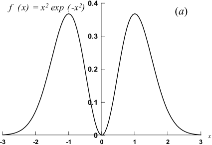
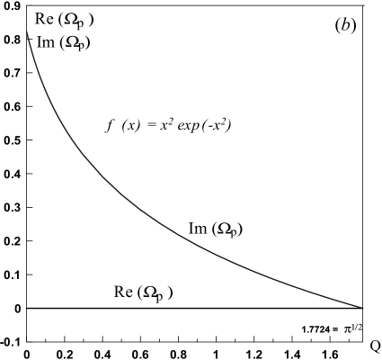
where for a distribution with a loss cone, i.e. with a deficiency of stars with low angular momenta, the DF $f(\nu)$ has a zero minimum at $\nu=0$:

$$f(0)=0,\quad f^{\prime}(0)=0,\quad f^{\prime\prime}(0)>0.$$ (3.11)

We assume that this minimum is unique, and the DF looks like what is shown in Figs. 4 or 5. An important point is that the quantity $Q$ in Eq. (3.10) is positive only when the orbit precession is retrograde. It is this circumstance that allows us to lean upon the analogy with plasma and use the formalism of the plasma theory when studying the instability. Recall that for the case of direct precession, when $Q<0$, Eq. (3.10) describes only the radial orbit instability (the modification of the Jeans instability for very elongated orbits) leading to the spokes merging together (Polyachenko & Shukhman, 1972; Antonov, 1973). Based on the Penrose – Nyquist criterion (see, e.g., Penrose 1960, or Mikhailovsky 1974), Polyachenko (1991b) showed that a new instability must occur in systems of orbits with retrograde precession. Here we reproduce this proof using a somewhat different language which is more physically evident and even more constructive: e.g., it allows us to determine, in a relatively simple manner, the instability boundary in the parameter $Q$. This approach is based on considering neutral modes.

Figure 4: Loss-cone instability in disk. a – symmetric distribution over precession velocity (3.13) with $a=0$; b – dependence of ${\rm Re}(\Omega_{p})$ and ${\rm Im}(\Omega_{p})$ on parameter $Q$.

Figure 5: The same as in Fig. 4 for asymmetric distribution (3.13) with $a=0.5$.

The essence of the approach is as follows. Suppose that, when the parameter $Q$ changes, the initially stable system becomes unstable. This means that some value of $Q=Q_{c}$ exists for which a neutral mode appears. For such a neutral mode, the location of the resonance should coincide with an extremum of the DF $f(\nu)$ – otherwise Eq. (3.10) will have a pole on the real axis, bypassing which would necessarily result in an imaginary contribution into the right side of (3.10); so that Eq. (3.10) could not be fulfilled. For distribution with one minimum and two maxima, one can show that (i) a neutral mode with a resonance at the location of a higher maximum cannot exist; (ii) when one maximum is much higher than the other, and two maxima are sufficiently separated from each other, the neutral mode corresponding to the lower maximum is possible, this mode belonging to the same oscillation branch as the neutral mode related to the minimum of the DF (see Sec. 3.3). Consequently, for the neutral mode at the minimum, $\Omega_{p}=0$, while for the other neutral mode, $\Omega_{p}=u_{1}$, where $\nu=u_{1}$ is the location of the lower maximum.

Putting $\Omega_{p}=0$ in (3.10), we find the value of $Q=Q_{c}^{({\rm min})}$, for which the neutral mode connected with the minimum can exist:

$$Q_{c}=\int_{-\infty}^{\infty}d\nu\,\nu^{-1}\,{f^{\prime}(\nu)}=\int_{-\infty}^{\infty}d\nu\,\nu^{-2}\,{f(\nu)}.$$ (3.12)

Here we have no need to elucidate the meaning of these integrals. Due to the condition (3.11), they converge at $\nu=0$ in the ordinary sense. Obviously, the right side of (3.12) is positive. So $Q_{c}^{({\rm min})}$ always exists, for arbitrary locations and heights of maxima. As to the sign of $Q_{c}^{({\rm max})}$, it can be either (as mentioned above). If it is positive, the second neutral mode exists. Note in addition that one more neutral mode, with $Q_{c}=0$ always exists; formally, it corresponds to the resonance at infinity.

With a knowledge of the values of $Q_{c}$ for neutral modes, one can determine domains of instability in the parameter $Q$ ($Q>0$) as $Q_{c}$ are the margin values. For this purpose, let us apply the perturbation theory.

First we consider the region near the boundary $Q=Q_{c}^{({\rm min})}$. Let us deflect from critical value: $Q=Q_{c}^{({\rm min})}+\delta Q$. The frequency $\Omega_{p}$ acquires an addition $\delta\Omega_{p}$, which is simply equal to $\Omega_{p}$. We would like to find out what direction should be taken to reach instability. Varying the quantity $Q$ relative to $Q_{c}^{({\rm min})}$ and $\Omega_{p}$ relative to zero in (3.10): $\delta Q=\delta\Omega_{p}\int_{-\infty}^{\infty}d\nu\,\nu^{-2}\,{f^{\prime}(\nu)}$. Here the pole in the integral must be bypassed below. This gives

$$\delta Q=\delta\Omega_{p}\,\bigl{[}\int\limits_{-\infty}^{\infty}-\ d\nu\,\nu^{-2}\,{f^{\prime}(\nu)}+i\pi f^{\prime\prime}(0)\bigr{]}.$$

Denoting $A=\displaystyle{\int\limits_{-\infty}^{\infty}}-\ d\nu\,\nu^{-2}\,{f^{\prime}(\nu)},\ \ B=\pi f^{\prime\prime}(0)>0,$ we obtain

$$\Omega_{p}=\delta\Omega_{p}={\delta Q}/(A+i\,B)=\bigl{[}(A-i\,B)/(A^{2}+B^{2})\bigr{]}\,\delta Q.$$

As $B>0$, the instability appears when $Q$ decreases below the critical value $Q_{c}^{({\rm min})}$.

For the second neutral mode (with the resonance at the location of lower maximum), we use the same procedure of the perturbation theory to find that the instability is possible when $Q$ is above the critical value $Q_{c}^{({\rm max})}$, as $B=\pi\,f^{\prime\prime}(u_{1})<0$ in the maximum.

As a result, we conclude that in the absence of the neutral mode associated with the lower maximum, i.e. if $Q_{c}^{({\rm max})}<0$, the unstable domain lies in the range $0<Q<Q_{c}^{({\rm min})}$. If such a neutral mode exists, the range of instability becomes $Q^{({\rm max})}<Q<Q_{c}^{({\rm min})}$. (It can be shown that $Q_{c}^{({\rm max})}<Q_{c}^{({\rm min})}$).

As for the question of where the resonance shifts when the parameter $Q$ is deflected from the corresponding margin value into the unstable domain, it depends on the sign of $A$, defined by the integrals in the sense of principal value. In principle, these integrals can have any sign. In the particular case of symmetric DF, showed in Fig. 4, the quantity $A$ is zero (for $Q$ deviating into the domain $Q<Q_{c}^{(\min)}$). Stability (or instability) is governed only by the sign of $B$, and this does not depend on the sign of $A$, which can be associated with the angular momentum of the wave.

We would like to say in this connection that here it is impossible to consider our instability in terms of exchanged angular momentum between the wave and the resonance stars, as is done in plasma physics or in the theory of galactic structures which has undergone appreciable development since the well-known paper by Lynden-Bell and Kalnajs (1972). The language for explaining the instability uses considerations operating with the momentum exchange between the wave and resonance stars. For instance, if the wave momentum is positive and the resonance stars lose their momentum transferring it to the wave, the momentum of the latter increases. This is the instability. However, such a language does not work in the case under consideration. The reason is that our systems are not weakly-dissipative, as is usual in plasma. In the latter we have a well-defined wave. All stars contribute into the wave dispersion properties, while the dissipation is determined by a small portion of resonant stars. Consequently, the dissipation is only a small correction. But now we have a completely different situation: the dissipation and dispersion parts of the wave (i.e., roughly speaking, the imaginary and real parts of dielectric permittivity) are of the same order. So our instability is not kinetic, in the ordinary sense, and such considerations do not work. However, in the case when the maxima are sufficiently separated, and their heights strongly differ from each other, we return to the usual, weakly-dissipative situation. Then the sign of phase velocity (i.e., the sign of $A$) must correlate with the inclination of the DF. In the following Sec. 3.3, we consider this case as well.

3.3 Neutral modes with resonance at DF maxima. Investigation of stability in a model two-humped distribution

To illustrate the above reasoning, we shall study a model example with DF

$$f_{a}(\nu)=(\nu^{2}/\nu_{T})\,\exp\,[-(\nu-a\nu_{T})^{2}/\nu_{T}^{2}]\\ \equiv\nu_{T}\,x^{2}\,\exp[-(x-a)^{2}],$$ (3.13)

where we can control the maximum locations and heights.

But first we shall prove the statement formulated in the preceding subsection that $Q_{c}$ for the neutral mode related to the higher maximum is always negative, while $Q_{c}$ for the lower maximum can have any sign. Suppose that the distribution has one maximum, similar to that showed in Fig. 4. Let the left maximum be at $\nu=u_{1}$, and the right maximum at $\nu=u_{2}$, the right maximum being larger than the left one: $f(u_{1})<f(u_{2})$. We shall consider these two variants separately.

(i) First let us assume that the neutral mode has frequency $\Omega_{p}=u_{2}$. Let us rewrite (3.10) in the form

$$Q_{c}^{({\rm max})}=\int\limits_{-\infty}^{\infty}d\nu\,\frac{d\,f(\nu)/{d\nu}}{\nu-u_{2}}=\int\limits_{-\infty}^{\infty}d\nu\,\frac{[f(\nu)-f(u_{2})]^{\prime}}{\nu-u_{2}}=\\ =\int\limits_{-\infty}^{\infty}d\nu\,\frac{[f(\nu)-f(u_{2})]}{(\nu-u_{2})^{2}}.$$ (3.14)

Note that all integrals here can be considered in the usual sense since no problems arise concerning their convergence at $\nu=u_{2}$. Since for the higher maximum, $\nu=u_{2}$, $f(\nu)<f(u_{2})$ everywhere, then the right side of (3.14) is obviously negative. Thus, we proved that there cannot be a neutral mode related to the higher maximum.

(ii) Let us now suppose that $\Omega_{p}=u_{1}$. Let us split the integral into two parts:

$$Q_{c}^{({\rm max})}=\int\limits_{-\infty}^{0}d\nu\,\frac{d\,f(\nu)/{d\nu}}{\nu-u_{1}}+\int\limits_{0}^{\infty}d\nu\,\frac{d\,f(\nu)/{d\nu}}{\nu-u_{1}}=\\ =\int\limits_{-\infty}^{0}d\nu\,\frac{[f(\nu)-f(u_{1})]}{(\nu-u_{1})^{2}}+\int\limits_{0}^{\infty}d\nu\,\frac{f(\nu)}{(\nu-u_{1})^{2}}.$$

Obviously, the integrals in the right side have opposite signs, so that the resulting sign can be either. In the case of the model (3.13), the quantity $Q_{c}^{({\rm max})}$ can be readily calculated:

$$Q_{c}^{({\rm max})}(a)=2\sqrt{\pi}\,\,[\,a\sqrt{\textstyle\frac{1}{4}\,a^{2}+1}-\textstyle\frac{1}{2}\,(a^{2}+1)],$$

so that at $a>a_{c}=2^{-1/2}\approx 0.71$, the quantity $Q_{c}^{({\rm max})}(a)$ becomes positive. Note that in the given model, $Q_{c}^{({\rm min})}$ does not depend on $a$ and equals $\sqrt{\pi}$.

Fig. 4 shows the dimensionless complex phase velocity of the wave, $\Omega_{p}$, as a function of $Q$ (in units of $\nu_{T}$, for the model (3.13) with $a=0$. It is evident that owing to symmetry the real part of the frequency $\Omega_{p}$ (and the quantity $A$ as well) is equal to zero.

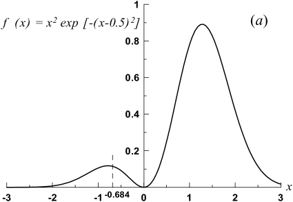
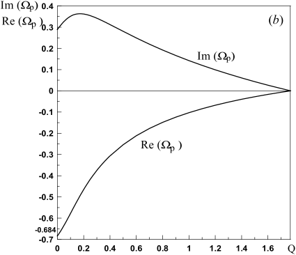
Fig. 5 shows $\Omega_{p}(Q)$ for the model (3.13) with $a=0.5$. Since $a<a_{c}$, then this model (as is the case with the model with $a=0$) sees only a neutral mode related to the minimum. As the model is asymmetric, the real part of the frequency is not zero. It is negative for $|\delta Q|\ll 1$ as $A>0$. Calculation shows that it remains negative when $Q$ is far from the instability boundary.

For sufficiently large values of $a$ ($a>a_{c}=1/\sqrt{2}$), the DF maxima (3.13) will be highly separated, and one of them becomes much higher than the other. Then $Q_{c}^{({\rm max})}$, for the neutral mode corresponding to the lower maximum, becomes positive, and a second neutral mode appears. As a result, the instability domain looks like a horizontal band (converging with increasing $a$), between these two neutral modes (see Fig. 6). Fig. 7 shows the tracks of a complex eigenvalue $x_{0}$ in a complex $x_{0}$-plane for various values of $a$. When the parameter $Q$ decreases from $Q^{({\rm min})}=\pi^{1/2}$ to $Q^{({\rm max})}(a)$ the position of the point on the corresponding curve changes so that ${\rm Re}(x_{0})$ moves from 0 to $x_{\rm max}(a)$, where $x_{\rm max}(a)$ is the position of the lower maximum, while ${\rm Im}(x_{0})>0$ and tends to zero on both ends of the curve.

Figure 6: Unstable region on $Q$ – $a$ - plane for the model (3.13) is bounded from above by the straight line $Q=Q_{c}^{({\rm min})}=\sqrt{\pi}$, from below by the curve $Q_{c}^{({\rm max})}(a)=2\sqrt{\pi}\,\,[\,a\sqrt{\frac{1}{4}\,a^{2}+1}-\frac{1}{2}\,(a^{2}+1)]$ (shaded).

Based on the plasma analogy, there is no difficulty in understanding the physical essence of the instability under sufficiently large values of $a$. When $a\gg 1$, the DF becomes identical to the DF of plasma particles with a weak beam moving at a rate significantly higher than the thermal velocity of particles in the main plasma (a beam at the tail). Then the instability degenerates into the well-known beam instability. It occurs when the wave phase velocity is on the slope of the beam DF oriented towards the main plasma. For our model (3.13) with $a>0$ the phase velocities of unstable modes must be negative, which is the case in our calculations (see Fig. 7).

Figure 7: The tracks of eigenvalue $x_{0}$ in complex $x_{0}$-plane for various values $a$, indicated near corresponding curves.

4 Loss-cone instability in spherically-symmetric systems

4.1 Basic set of integral equations

As we did in the case of disks, here we start with an exact equation governing perturbations in a spherical system with DF $F=F(E,L)$, where $E=\frac{1}{2}\,v_{r}^{2}+\frac{1}{2}\,{L^{2}}/{r^{2}}+\Phi_{0}(r)$ is the star energy, $L=rv_{\bot}\equiv r\,(v_{\theta}^{2}+v_{\varphi}^{2})^{1/2}$ is the absolute value of angular momentum, $\Phi_{0}(r)$ is the unperturbed gravitational potential. We assume that the DF does not depend on the third integral $L_{z}=rv_{\varphi}\sin\theta$. As is well-known, the spectrum of eigenvalues $\omega$ in this case is independent of the azimuthal number $m$. Thus, instead of a general representation of the potential and density in the form of the sectorial harmonic $\Phi(t;r,\theta,\varphi)=\chi(r)\,Y_{l}^{m}(\theta,\phi)\,e^{-i\omega t}$ and $\rho(t;r,\theta,\varphi)={\hat{\rho}}(r)\,Y_{l}^{m}(\theta,\phi)\,e^{-i\omega t}$, we can restrict our consideration to a simpler variant $\Phi(t;r,\theta,\varphi)=\chi(r)\,P_{l}(\cos\theta)\,e^{-i\omega t},\ \ \rho(t;r,\theta,\varphi)={\hat{\rho}}(r)\,P_{l}(\cos\theta)\,e^{-i\omega t},$ where $P_{l}(x)$ is the Legendre polynomial. The derivation of the basic integral equation (a set of integral equations, to be precise) is also based on the action–angle formalism (as in the disk case) and presented in Appendix A. Note that this formalism was first used in the paper by Polyachenko & Shukhman (1981) as applied to spherical gravitating systems.

Thus, the initial exact set of integral equations has the form ($l_{1},l^{\prime}_{1}=-\infty,\dots,\infty$; $l_{2},l^{\prime}_{2}=-l,\dots,l$):

$$\chi_{\,l_{1},\,l_{2}}(E,L)=\frac{4\pi G}{2l+1}\sum\limits_{l_{1}^{\prime}=-\infty}^{\infty}\sum\limits_{l_{2}^{\prime}=-l}^{l}D_{l}^{l_{2}^{\prime}}\int\frac{dE^{\prime}\,LdL^{\prime}}{\Omega_{1}(E^{\prime},L^{\prime})}\\ \times\chi_{\,l_{1}^{\prime}\,l_{2}^{\prime}}(E^{\prime},L^{\prime})\,\Pi_{l_{1},\,l_{2};\,l_{1}^{\prime},\,l_{2}^{\prime}}(E,L;E^{\prime},L^{\prime})\times\\ \times\,\frac{\Bigl{[}\,l_{1}^{\prime}\,\Omega_{1}(E^{\prime},L^{\prime})+l_{2}^{\prime}\,\Omega_{2}(E^{\prime},L^{\prime})\Bigr{]}\,{\partial F}/{\partial E^{\prime}}+l_{2}^{\prime}\,{\partial F}/{\partial L^{\prime}}}{\omega-l_{1}^{\prime}\,\Omega_{1}(E^{\prime},L^{\prime})-l_{2}^{\prime}\,\Omega_{2}(E^{\prime},L^{\prime})}$$ (4.1)

with the kernel

$$\Pi_{l_{1},\,l_{2};\,l_{1}^{\prime},\,l_{2}^{\prime}}(E,L;E^{\prime},L^{\prime})\\ =\int\limits_{0}^{2\pi}dw_{1}\int\limits_{0}^{2\pi}dw_{1}^{\prime}\,{\cal F}_{l}\left[\,r\,(E,L;w_{1}),r^{\prime}(E^{\prime},L^{\prime};w_{1}^{\prime})\right]\times\\ \times\exp{\left\{\,i\left[\Bigl{(}\,l_{1}^{\prime}\,w_{1}^{\prime}+l_{2}^{\prime}\,{\partial S_{1}}/{\partial I_{2}^{\prime}}\Bigr{)}-\Bigl{(}l_{1}\,w_{1}+l_{2}\,{\partial S_{1}}/{\partial I_{2}}\Bigr{)}\right]\right\}}.$$ (4.2)

This is a two-dimension set of integral equations relative to unknown functions $\chi_{l_{1},\,l_{2}}(E,L)$, which are related to the radial part of perturbed potential by

$$\chi_{l_{1},\,l_{2}}(E,L)=\int\limits_{0}^{2\pi}e^{-(l_{1}w_{1}+l_{2}\partial S_{1}/\partial I_{2})}\chi\bigl{[}r(E,L,w_{1})\bigr{]}\,dw_{1}.$$ (4.3)

In Eq. (4.1), we denote

$$D_{l}^{k}=\left\{\begin{array}[]{cc}\dfrac{1}{2^{\,2\,l}}\,\dfrac{(l+k)!\,\,(l-k)!}{\left[\Bigl{(}\frac{1}{2}\,(l-k)\Bigr{)}!\,\Bigl{(}\frac{1}{2}\,(l+k)\Bigr{)}!{\phantom{\bigg{|}}}\right]^{2}},&|l-k|\ {\rm even},\\ \\ 0&|l-k|\ \ {\rm odd}.\end{array}\right.$$ (4.7)

In Eq. (4.2)

$${\cal F}_{l}(r,r^{\prime})=\frac{(r_{<})^{l}}{(r_{>})^{l+1}},\ \ r_{<}={\rm min}(r,r^{\prime}),\ \ r_{>}={\rm max}(r,r^{\prime}),$$

while the function of radial action $S_{1}$ in (4.2) and (4.3) is

$$S_{1}=\int\limits_{r_{\rm min}}^{r}dr^{\prime}\sqrt{2E\,({\mbox{\boldmath$I$}})-2\Phi_{0}(r^{\prime})-{(I_{2}+|I_{3}|)^{2}}/{r^{\prime 2}}\phantom{\big{|}}},\ \$$

where ${\mbox{\boldmath$I$}}=(I_{1},I_{2},I_{3})$ and the actions $I_{2}$ and $I_{3}$ are related to the integrals of motion $L$ and $L_{z}$ by $\ L=I_{2}+|I_{3}|,\ L_{z}=I_{3}$. The dependence $r\,(E,L;w_{1})$ is determined from

$$w_{1}={\partial S_{1}}/{\partial I_{1}}=\Omega_{1}\int\limits_{r_{\rm min}}^{r}\frac{dr^{\prime}}{\sqrt{2E-2\Phi_{0}(r^{\prime})-{L^{2}}/{r^{\prime 2}}\phantom{\big{|}}}}.$$

We should also keep in mind that indices $l_{1}$ and $l_{2}$ correspond to the spatial dependence of the perturbed potential expanded over harmonics of the angular variables $w_{1}$ and $w_{2}$, conjugate to the action variables

$$I_{1}=\frac{1}{2\pi}\oint p_{r}\,dr=\frac{1}{\pi}\int_{r_{\rm min}}^{r_{\rm max}}\sqrt{2E-2\Phi_{0}(r)-L^{2}/r^{2}\phantom{\big{|}}}dr,$$

$$I_{2}=\frac{1}{2\pi}\oint p_{\theta}\,d\theta=\frac{1}{\pi}\int_{\theta_{0}}^{\pi-\theta_{0}}\sqrt{L^{2}-L_{z}^{2}/\sin^{2}\theta}=L-|L_{z}|,$$

respectively:

$$\Phi({\mbox{\boldmath$I$}},w_{1},w_{2})=(2\pi)^{-2}\sum\Phi_{\,l_{1},\,l_{2}}({\mbox{\boldmath$I$}})\,e^{i\,(\,l_{1}\,w_{1}+l_{2}\,w_{2})}.$$

In the case of $m=0$, the dependence on the angular variable $w_{3}$ is absent. Let us also give an alternative form for ${\cal F}_{l}(r,r^{\prime})$ (sometimes it proves to be more convenient):

$${\cal F}_{l}(r,r^{\prime})=(2l+1)\int\limits_{0}^{\infty}dk\,\frac{J_{\,l+{1}/{2}}(kr)}{\sqrt{k\,r}}\,\frac{J_{\,l+{1}/{2}}(kr^{\prime})}{\sqrt{k\,r^{\prime}}},$$ (4.8)

where $J_{\nu}(x)$ is a Bessel function (see Polyachenko & Shukhman 1982).

4.2 Simplified equation for describing slow modes

Let us assume that a massive nucleus or a black hole (with mass $M_{c}$) is placed at the galactic center. Moreover, we assume that the central mass dominates the unperturbed potential $\ \Phi_{0}(r)$, so that $\ \Phi_{0}(r)=\Phi_{c}(r)+\Phi_{G}(r),$ where $\Phi_{c}(r)=-{GM_{c}}/{r}$, $\Phi_{G}(r)$ is the potential created by the spherical subsystem of galaxy. Then the force acting on a star from the central mass significantly exceeds the force from stars in the galactic spherical component: $|\Phi_{c}^{\prime}(r)|\gg|\Phi_{G}^{\prime}(r)|.$ In this case, stellar orbits are predominately governed by the potential of the central massive point. This means that we are dealing with 1:1-type orbits. Due to a small additional potential $\Phi_{G}(r)$, the Keplerian ellipses precess, the precession velocity is determined by the small difference $\ \Omega_{\rm pr}(E,L)=\Omega_{2}(E,L)-\Omega_{1}(E,L),\ \Omega_{\rm pr}\ll\Omega_{1}\approx\Omega_{2}.$

An explicit expression for the precession velocity in terms of the potential $\Phi_{G}(r)$ was found in the Section 2 (see formula (2.8)). We shall be interested in slow modes, i.e., modes with frequencies of the order of precession velocities, $\omega={\cal O}(\Omega_{\rm pr})$. Then from all items with denominators $\bigl{[}\omega-l^{\prime}_{1}\,\Omega_{1}(E^{\prime},L^{\prime})-l^{\prime}_{2}\,\Omega_{2}(E^{\prime},L^{\prime})\bigr{]}$, we keep only those with $l_{1}^{\prime}=-l_{2}^{\prime}$. These denominators can be transformed into ${\omega-l_{1}^{\prime}\,\Omega_{1}(E^{\prime},L^{\prime})-l_{2}^{\prime}\,\Omega_{2}(E^{\prime},L^{\prime})}={\omega-l_{2}^{\prime}\,\Omega_{\rm pr}(E^{\prime},L^{\prime})}$. The frequency constructions in numerators of these contributions are equal to

$$\Bigl{[}\,l_{1}\,\Omega_{1}(E^{\prime},L^{\prime})+l_{2}^{\prime}\,\Omega_{2}(E^{\prime},L^{\prime})\Bigr{]}{\partial F}/{\partial E^{\prime}}+{\partial F}/{\partial L^{\prime}}\\ =l_{2}^{\prime}\,\left[\Omega_{\rm pr}(E^{\prime},L^{\prime})\,{\partial F}/{\partial E^{\prime}}+{\partial F}/{\partial L^{\prime}}\right].$$ (4.9)

The expression in square brackets is a so-called Lynden-Bell derivative (Lynden-Bell, 1979) of the DF:

$$\left({\partial F}/{\partial E}\right)_{L}\Omega_{\rm pr}+\left({\partial F}/{\partial L}\right)_{E}=\left({\partial F}/{\partial L}\right)_{LB}.$$ (4.10)

Recall that it is defined as the derivative with respect to the absolute value of angular momentum, $L=I_{2}+|I_{3}|$, with the adiabatic invariant, $J_{f}=I_{1}+I_{2}+|I_{3}|$, and the projection of angular momentum, $L_{z}$, being constant.

Denoting

$$\chi(E,L)_{l_{1}=-l_{2},\,l_{2}}=\phi_{l_{2}}(E,L),\\ \Pi_{l_{1}=-l_{2},\,l_{2};\,l_{1}^{\prime}=-l_{2}^{\prime},\,l_{2}^{\prime}}(E,L;E^{\prime},L^{\prime})=P_{l_{2},\,l_{2}^{\prime}}(E,L;E^{\prime},L^{\prime})$$

and keeping only items with $l_{1}^{\prime}=-l_{2}^{\prime}$ in the sum (4.1) over $l_{1}^{\prime}$, we find a “slow” equation for quantities $\phi_{n}(E,L)$:

$$\phi_{n}(E,L)=\dfrac{4\pi G}{2l+1}\sum\limits_{n^{\prime}=-l}^{l}D_{l}^{n^{\prime}}\int\dfrac{dE^{\prime}\,L^{\prime}dL^{\prime}}{\Omega_{1}(E^{\prime},L^{\prime})}\\ \times\,P_{\,n;\,n^{\prime}}(E,L;E^{\prime},L^{\prime})\,\dfrac{n^{\prime}\,\left({\partial F}/{\partial L^{\prime}}\right)_{LB}}{\omega-n^{\prime}\,\Omega_{\rm pr}(E^{\prime},L^{\prime})}\,\phi_{\,n^{\prime}}(E^{\prime},L^{\prime}),$$ (4.11)

with the kernel

$$P_{\,n,\,n^{\prime}}(E,L;E^{\prime},L^{\prime})=\\ =\int\limits_{0}^{2\pi}dw_{1}\int\limits_{0}^{2\pi}dw_{1}^{\prime}\,{\cal F}_{\,l}\left[\,r\,(E,L;w_{1}),r^{\prime}(E^{\prime},L^{\prime};w_{1}^{\prime})\right]\times\\ \times\exp{\left\{\,i\left[n^{\prime}\,\Bigl{(}{\partial S_{1}}/{\partial I_{2}^{\prime}}-w_{1}^{\prime}\Bigr{)}-n\,\Bigl{(}{\partial S_{1}}/{\partial I_{2}}-w_{1}\Bigr{)}\right]\right\}}.$$

The kernel $P_{\,n,\,n^{\prime}}$ can be rewritten in an explicitly real form if one changes the limits of integration over $w_{1}$ and $w_{1}^{\prime}$ from $[0,2\pi]$ to $[-\pi,\pi]$. Then it becomes evident that $r(w_{1},E,L)$ is the symmetric function of $w_{1}$, and

$$P_{\,n,\,n^{\prime}}(E,L;E^{\prime},L^{\prime})=\\ 4{\displaystyle\int\limits_{0}^{\pi}}dw_{1}{\displaystyle\int\limits_{0}^{\pi}}dw_{1}^{\prime}\,{\cal F}_{\,l}\left[\,r\,(E,L;w_{1}),r^{\prime}(E^{\prime},L^{\prime};w_{1}^{\prime})\right]\\ \times\cos\left[n^{\prime}\,\Bigl{(}{\partial S_{1}}/{\partial I_{2}^{\prime}}-w_{1}^{\prime}\Bigr{)}\right]\,\cos\left[n\,\Bigl{(}{\partial S_{1}}/{\partial I_{2}}-w_{1}\Bigr{)}\right].$$

The quantity $\phi_{\,n}(E,L)$ can also be written in a simpler form

$$\phi_{\,n}(E,L)=2{\displaystyle\int\limits_{0}^{\pi}}\cos\left[\,n\,\Bigl{(}{\partial S_{1}}/{\partial I_{2}}-w_{1}\Bigr{)}\right]\,\chi\,\bigl{[}r(E,L,w_{1})\bigr{]}\,dw_{1}.$$

4.3 Simplified equation for the case of nearly radial orbits

In the case of orbits with low angular momenta $L$ we are interested in the set of equations (4.11) for slow modes allows further significant simplifications. The requirements imposed on the width, $\delta L$, of localization domain of the DF in angular momentum were discussed in Sec. 3.

Based on the fact that the kernel $P_{n\,n^{\prime}}(E,L;E^{\prime},L^{\prime})$, for nearly radial orbits, depends only on energies $E$ and $E^{\prime}$ (accurate to terms quadratic in $L$ and $L^{\prime}$) and acquires the form $\ P_{n\,n^{\prime}}(E,L;E^{\prime},L^{\prime})\approx P_{n\,n^{\prime}}(E,0;E^{\prime},0^{\prime})=(-1)^{n+n^{\prime}}\Pi(E,E^{\prime}),\$ where

$$\Pi(E,E^{\prime})=4\int\limits_{0}^{\pi}dw_{1}\int\limits_{0}^{\pi}dw_{1}^{\prime}\,{\cal F}_{l}[\,r(E,w_{1}),r^{\prime}(E^{\prime},w_{1}^{\prime})]=\\ =4\Omega_{1}(E)\,\Omega_{1}(E^{\prime})\!\!\int\limits_{0}^{b(E)}\dfrac{dr}{v_{r}(E,r)}\int\limits_{0}^{b(E^{\prime})}\dfrac{dr}{v_{r}(E^{\prime},r^{\prime})}\,\,{\cal F}_{\,l}(r,r^{\prime}),$$ (4.12)

$\Omega_{1}(E)={(2|E|)^{3/2}}/(GM_{c})$, $b(E)\equiv r_{\rm max}(E)={GM_{c}}/{|E|}$, $v_{r}(E,r)=\sqrt{2|E|}\,\sqrt{(b-r)/{r}}.$ The unknown function $\phi_{n}(E,L)$ also depends only on $E$ (accurate to ${\cal O}(L^{2})$): $\ \phi_{n}(E,L)\approx(-1)^{n}\Phi(E).$ Moreover, according to (4.10), the Lynden-Bell derivative in $L$ coincides (accurate to ${\cal O}\bigl{[}(M_{G}/M_{c})\,L^{2}\bigr{]}$) with the derivative in $L$, with the energy $E$ constant. As a result the equation (4.11) transforms into the one-dimension integral equation

$$\Phi(E)=\dfrac{4\pi G}{2l+1}\int\int\dfrac{dE^{\prime}\,L^{\prime}dL^{\prime}}{\Omega_{1}(E^{\prime})}\,\Pi(E,E^{\prime})\,\Phi(E^{\prime})\\ \times\sum\limits_{s\,=-\,l}^{l}s\,D_{l}^{s}\,\dfrac{\partial F(E^{\prime},L^{\prime})/\partial L^{\prime}}{\omega-s\,\varpi(E^{\prime})\,L^{\prime}}.$$ (4.13)

4.4 Model case of monoenergetic distribution

Let us consider again the model distribution $F(E,L)=f(L)\,\delta(E-E_{0})$, as in the disk case. Integrating (4.13) over $E^{\prime}$ and putting $E=E_{0}$ in the resulting equation, we obtain the characteristic equation in the form

$$1=\dfrac{4\pi G}{2l+1}\dfrac{\Pi(E_{0},E_{0})}{\Omega_{1}(E_{0})}\,\,\int L\,dL\sum\limits_{s\,=-\,l}^{l}s\,D_{l}^{s}\,\dfrac{df(L)/dL}{\omega-s\,\varpi(E_{0})\,L}.$$

Recall (see Sec. 2) that for the case of near-Keplerian orbits (i.e., orbits of the 1:1 type), the orbit precession is retrograde for arbitrary distributions of the potential $\Phi_{G}(r)$, i.e., $\varpi<0$.

For convenience, we can turn from the variable $L$ to the variable $\nu=|\Omega_{\rm pr}|=|\varpi(E_{0})|L=-\varpi L>0$. Denoting $f(L)=f\bigl{(}{\nu}/{|\varpi|}\bigr{)}\equiv f_{0}(\nu),$ we write

$$1=-\dfrac{4\pi G}{2l+1}\dfrac{\Pi(E_{0},E_{0})}{|\varpi(E_{0})|\Omega_{1}(E_{0})}\,\,\int\nu\,d\nu\sum\limits_{s\,=-\,l}^{l}s\,D_{l}^{s}\,\dfrac{df_{0}(\nu)/d\nu}{\omega-s\,\nu}.$$ (4.14)

The equation (4.14) coincides with the Eq. (2) of Polyachenko (1991a), derived immediately in the spoke approximation The rather cumbersome derivation above provides the basis for the spoke approach (together with the one for disks, in the previous Section).

To conclude this subsection, let us note that the monoenergetic model under consideration corresponds to the specific density distribution of spherical cluster $\rho_{0}(r)$ (and the potential $\Phi_{G}(r)$) and has the finite radius $R={GM_{c}}/{|E_{0}|}$. For this distribution, the quantity $\varpi(E_{0})$ can be explicitly calculated:

$$\varpi(E_{0})=-\frac{M_{G}}{M_{c}}\,\frac{8}{\pi^{2}}\,\frac{1}{R^{2}}.$$ (4.15)

Here $M_{G}$ is the total mass of the spherical cluster (recall that it is assumed that $M_{G}\ll M_{c}$). The kernel $\Pi(E_{0},E_{0})$ can also be calculated in the explicit form. Using the relations (4.8) and (4.12), we obtain

$${\Pi}(E_{0},E_{0})=\frac{8\pi^{2}(2\,l+1)}{R}\,C_{l},\ \ \\ C_{l}=\int\limits_{0}^{\infty}\frac{dz}{z}\,\left[J_{\,(\,l+1)/2}(z)J_{\,l/2}(z)\right]^{2}.$$ (4.16)

The first seven coefficients $C_{l}$ calculated from (4.16) are presented in Table 1. After substituting these coefficients into (4.14), we find

$$1=-{\cal A}_{l}\int\nu\,d\nu\sum\limits_{s\,=-\,l}^{l}s\,D_{l}^{s}\,\dfrac{d\,f_{0}(\nu)/d\nu}{\omega-s\,\nu},\\ {\cal A}_{l}=\frac{16\pi^{3}\,G\,C_{l}}{|\varpi|}\,\left(\frac{R}{2GM_{c}}\right)^{1/2}.$$ (4.17)

This equation can also be written in the form

$$1=-2{\cal A}_{l}\sum\limits_{s\,=1}^{l}s^{2}\,D_{l}^{s}\,\int d\nu\,\dfrac{\nu^{2}d\,f_{0}(\nu)/d\nu}{\omega^{2}-s^{2}\,\nu^{2}}.$$ (4.18)

The DF $f_{0}(\nu)$ is normalized by the condition that the total mass of spherical cluster is equal to $M_{G}$, i.e., $\int Fd\,\Gamma=M_{G}$. This gives

$$\int f_{0}(\nu)\,\nu\,d\nu={\textstyle\frac{1}{2}}\,(2\pi)^{-3}\,[\varpi(E_{0})]^{2}\Omega_{1}(E_{0})M_{G}.$$ (4.19)

$l$	1	2	3	4	5	6	7
$C_{l}$	0.135	0.063	0.037	0.025	0.018	0.014	0.011

Table 1: The values of coefficients $C_{l}$.

4.5 Stability of the $l=1$ and $l=2$ modes

We begin with studying the stability of modes $l=1$ and $l=2$. As we shall show, these modes are stable. For definiteness, let us take the mode $l=2$. From the considerations below, it will be immediately obvious that they are valid for the mode $l=1$ as well.

We start with the equation (4.18) for the mode $l=2$. An important point is that (4.18) for this mode (as with $m=1$) includes only one item in the sum over $s$ (with $s=2$) (correspondingly, two items $s=\pm 2$ in (4.17)). This follows from definition (4.7) of the quantity $D_{l}^{s}$ and the equation (4.18). For $l=2$, $D_{2}^{2}={\textstyle\frac{3}{8}}$, so that

$$Q=-4\int\limits_{0}^{\infty}\dfrac{\nu^{2}\,\bigl{[}d\,f_{0}(\nu)/d\nu\,\bigr{]}}{\omega^{2}-4\,\nu^{2}}\,d\nu,\ \ \ Q={\textstyle\frac{4}{3}}\,{\cal A}_{2}^{-1}>0.$$ (4.20)

Let the DF has a beam-like form due to deficiency of stars with low angular momenta or, which is the same, with small precession velocities $\nu$. We assume that the distribution has only one maximum, located at $\nu=u$ on the semi-axis $0\leq\nu<\infty$. If there is a neutral mode, at some value of $Q=Q_{c}$, the corresponding resonance must coincide with the maximum of $f_{0}(\nu)$, i.e., $\omega^{2}=4u^{2}$. This means that for $Q=Q_{c}$

$$Q_{c}=-\int\limits_{0}^{\infty}\dfrac{\nu^{2}\,\bigl{[}d\,f_{0}(\nu)/d\nu\,\bigr{]}}{u^{2}-\nu^{2}}\,d\nu.$$ (4.21)

Evidently, for any one-hump distribution, the right side of (4.21) is negative, as the integrand is free of singularities and positive everywhere. Since $Q>0$, we conclude that the neutral mode is impossible. The absence of neutral mode means that the marginal value of $Q$, $Q=Q_{c}$, which separates stable and unstable distributions, is also absent: each distribution is either stable for all values of $Q$ or unstable everywhere. Since stable one-hump distributions obviously exist, we conclude that the mode $l=2$ is always stable.

The above considerations make it also clear that the conclusion about the stability of the mode $l=2$ is valid only for the case of retrograde precession, when the quantity $Q$ in Eq. (4.20) is positive. In the case of prograde precession, $Q<0$, so that the neutral mode (as well as the instability) exists. This is the well-known radial orbit instability. True, here it develops in a non-monotonic distribution with an empty loss cone, instead of the usual distributions when most stars are concentrated at near-radial orbits.

However, the conclusion that the instability is utterly impossible in the case of retrograde precession would be premature. The matter is that we obtain the above result concerning the mode $l=2$ due to a formal reason: for this mode there is only one summand in the sum over $s$. So, indeed, the instability is absent for $l=2$ (and $l=1$ as well). However, for modes with $l\geq 3$, when there are at least two summands in that sum, the instability becomes possible under suitable conditions. In the following subsection, we study the mode $l=3$ in detail and demonstrate that the instability can occur here.

4.6 The mode $l=3$

Considering the case of retrograde precession and restricting ourselves only to the mode $l=2$, we showed (Sec. 4.5) that neutral modes (and consequently the instability) are absent for one-hump distributions. However, this is valid only in the special case that the mode has one resonance, as with $l=2$ or $l=1$. Recall that the proof is based on the fact that the resonance must then be located at the DF maximum. In such a situation, the characteristic relation cannot be satisfied as the signs of right and left sides of (4.21) are necessarily opposite, when $\omega$ equals the frequency of neutral mode.

This proof, however, fails if a neutral mode has two (or more) resonances. Indeed, the resonances can then be located so that the resulting growth at one group of resonances is totally cancelled by an equal damping at another group. In these conditions, a neutral mode can exist. This means that the former group of resonances must be located right of the maximum while the latter group to the left. In the simplest case when there are only two resonances, we must conclude that these resonances necessarily lie on different sides of the maximum. Then it is hard to make a certain conclusion about the sign of the integrand in the characteristic relation that involves the principal value integrals, with a singularity at each resonance. One may hope therefore that we can find neutral modes (and consequently the instability) for $l\geq 3$ when there is at least a couple of resonances. Now we study the possibility of neutral mode in the simplest suitable case of $l=3$.

For $l=3$, we have $D_{3}^{1}=\frac{3}{16},\ \ \ D_{3}^{3}=\frac{5}{16}$. The characteristic equation (4.18) gives

$$Q=-\int\!d\nu\,\nu^{2}\,\frac{d\,f_{0}(\nu)}{d\nu}\left(\frac{1}{\omega^{2}-\nu^{2}}+\frac{15}{\omega^{2}-9\nu^{2}}\right)\!,\ Q={\textstyle\frac{8}{3}}\,{\cal A}_{3}^{-1}\!.$$ (4.22)

Let us suggest that the neutral mode with the frequency $\omega=\omega_{0}$ occurs at some value of $Q=Q_{c}$. For definiteness, we assume that $\omega_{0}>0$. For this frequency, there are two resonances:

$$\nu=\nu_{1}=\omega_{0},\ \ \ \nu=\nu_{2}={\textstyle\frac{1}{3}}\,\omega_{0}.$$ (4.23)

Obviously, the resonance corresponding to smaller $\nu$ (i.e., $\nu=\omega_{0}/3$), must lie to the left of the maximum of the function $f_{0}(\nu)$ (we denote its position $u$), while the resonance corresponding to larger $\nu$ (i.e., $\nu=\omega_{0}$), must lie to the right of the maximum: ${\textstyle\frac{1}{3}}\,\omega_{0}<u<\omega_{0}.$ Bypassing the singularity in the complex plane $\nu^{2}$ from below and equating the imaginary part of the full integral (4.22) to zero, we find

$$f_{0}^{\prime}(\omega_{0})+{\textstyle\frac{5}{9}}\,f_{0}^{\prime}\left({\textstyle\frac{1}{3}}\,\omega_{0}\right)=0.$$ (4.24)

Here we should explain that direction of bypassing in the complex plane $\nu^{2}$ coincides with that in the complex plane $\nu$ (i.e., it is from below) because of $\omega_{0}>0$. The condition (4.24) expresses the balance between growth at one of resonances and damping at the other. Eq. (4.24) determines the frequency of the neutral mode which exists when $Q=Q_{c}$, the latter found from the condition

$$Q_{c}=-\int-\ d\nu\,\nu^{2}\,\frac{d\,f_{0}(\nu)}{d\nu}\left(\frac{1}{\omega_{0}^{2}-\nu^{2}}+\frac{15}{\omega_{0}^{2}-9\nu^{2}}\right).$$ (4.25)

Eq. (4.25) involves the principal value integrals. The pair of equations, (4.24) and (4.25), determines the frequency of the neutral mode and the critical value of parameter $Q$, $Q=Q_{c}$ such that the system has a neutral mode. This is in fact the condition on some DF parameter (say, dispersion of precession velocities, $\nu_{T}$), or on mass, $M_{G}$, of spherical component (i.e., on value of its self-gravitation). Under this condition, the system is at the stability boundary. If the parameter deviates from its critical value in a certain direction, the system becomes unstable. This direction is yet to be determined.

It is not evident beforehand that the right side of Eq. (4.25) will be positive for potential neutral modes. (Their frequencies are determined from Eq. (4.24). It is easy to understand that for one-hump distributions, a suitable solution of this equation always exists.)

Moreover, we showed above for the mode $l=2$ (in fact, for the mode $l=1$ as well) that in principle the neutral modes are absent as the resulting value of $Q$ turns out to be negative.

In order to clarify the possibility of neutral modes $l\geq 3$ in more detail, we consider the series of specific models in the form of one-hump distributions $\ f_{0}^{(n)}(\nu)=N_{n}(\nu^{2})^{n}\,\exp\left(-{\nu^{2}}/{\nu_{T}^{2}}\right),$ where $N_{n}$ is the normalized coefficient, $n=1,2,...$ . On the assumption that the DF is normalized to some total mass ${\bar{M}}$ by the condition

$$\int_{0}^{\infty}\nu\,d\nu f_{0}^{(n)}={\bar{M}},$$ (4.26)

then $N_{n}=\bigl{[}2{\bar{M}}/(\nu_{T}^{2})^{n+1}\bigr{]}(n!)^{-1}$. Dimensionless variables are introduced for convenience: $x={\nu^{2}}/{\nu_{T}^{2}},\ \ x_{0}={\omega_{0}^{2}}/{\nu_{T}^{2}}$. Besides, we shall use the function $f_{n}(x)=f_{0}^{(n)}\left(\nu_{T}\sqrt{x}\right)=N_{n}\,(\nu_{T}^{2})^{n}\,\,x^{n}\,e^{-x}$, instead of the function $f_{0}^{(n)}(\nu)$. In new designations, the set of equations (4.24) and (4.25) takes the form

$$f_{n}^{\prime}(x_{0})+{\textstyle\frac{5}{27}}\,f_{n}^{\prime}\left({\textstyle\frac{1}{9}}\,x_{0}\right)=0,$$ (4.27)

$$Q_{c}=-\int\limits_{0}^{\infty}-\ dx\,\ x\,\frac{d\,f_{n}(x)}{dx}\left(\frac{1}{x_{0}-x}+\frac{15}{x_{0}-9x}\right),$$ (4.28)

where

$$f_{n}^{\prime}(x)=(N_{n}\,\nu_{T}^{2n})\,x^{n-1}(n-x)\,e^{-x}.$$ (4.29)

One can see from (4.29) that the maximum of the function $f_{n}(x)$ is located at $x=n$, so that (4.23) gives the condition on the value of dimensionless frequency squared: $n<x_{0}<9n$. The value $x_{0}$ is found from Eq. (4.27), that takes the form of a transcendental equation

$$(9n-x_{0})-{\textstyle\frac{1}{5}}\,3^{2n+3}\,\exp\left(-{\textstyle\frac{8}{9}}\,x_{0}\right)\,(x_{0}-n)=0.$$ (4.30)

It is evident that at least one root always exists as the left side of Eq. (4.30) has opposite signs at the ends of the interval under consideration. More detailed calculations (or plotting the left side) show that there are actually three roots satisfying the condition $n<x_{0}<9n$, for each $n$. All roots are candidates for a possible neutral mode. The numerical solution of Eq. (4.30), for $n=1,...,7$, gives squared dimensionless frequencies of neutral modes listed in Table 2.

$n$	$x_{0}^{(1)}$	$x_{0}^{(2)}$	$x_{0}^{(3)}$
1	1.66	3.44	8.85
2	2.27	5.343339	17.99
3	3.09	7.733736	26.99
4	4.03	10.17	35.99
5	5.01	12.63	44.99
6	–	15.09	–
7	–	17.55	–

Table 2: The values of squared dimensionless frequencies – candidates to neutral mode.

We next substitute the obtained values of $x_{0}$ into the relation (4.28) that determines $Q_{c}$. Let us represent it in the form convenient for numerical calculations. To do this, we introduce the function $g_{n}(x)$:

$$g_{n}(x)=e^{-x}\int\limits_{-\infty}^{x}-\ \frac{dt}{t}\,\,e^{\,t}\,\,[(x-t)^{n}\,(x-t-n)],\ \ \ \ x>0.$$

Using this function, Eq. (4.28) can be written as

$$\ {\bar{Q}}_{c}^{(n)}=g_{n}(x_{0})+{\textstyle\frac{5}{3}}\,\,g_{n}\left({\textstyle\frac{1}{9}}\,{x_{0}}\right),$$

where we denoted $\ {\bar{Q}}^{(n)}\equiv{Q}/[{\nu_{T}^{2n}\,N_{n}}]=n!\,({Q}/{2{\bar{M}}})\,\nu_{T}^{2},$ and the quantity ${\bar{M}}$ (see (4.26)) is determined by the normalization requirement for the monoenergetic model, (4.19), i.e.,

$$\ {\bar{M}}={\textstyle\frac{1}{2}}(2\pi)^{-3}\,\varpi(E_{0})^{2}\Omega_{1}(E_{0})\,M_{G}.$$

Substituting all three roots $x_{0}^{(1)},x_{0}^{(2)},x_{0}^{(3)}$ into (4.28), we obtain the following results.

(i). For the DF with $n=1$, the right side of (4.28) turns out to be negative for each potential neutral mode. This means that the mode $l=3$ has no neutral modes (consequently, the mode is stable) for the model $n=1$.

(ii). For the models with $n\geq 2$, there is one neutral mode. It corresponds to the middle root $x_{0}$ (in Table 2, it is the root $x_{0}^{(2)}$). Only for this root, the right side of (4.28) turns out to be positive. This means that these models can be unstable if the parameter $Q$ differs from the critical value we found. Recall that the deviation direction of $Q$ is yet to be determined. The critical values $Q_{c}^{(n)}$ are presented in Table 2.

Fig. 8 shows the resonances for the neutral mode in the model with $n=2$, for illustration. As is seen in Table 1, the dimensionless frequency $\omega_{0}/\nu_{T}$ is equal to $\sqrt{5.34}\approx 2.31$. So the resonances lie at $\nu/\nu_{T}=\omega_{0}/(3\nu_{T})=0.77$ and $\nu/\nu_{T}=\omega_{0}/\nu_{T}=2.31$.

Figure 8: Positions of resonances for the mode $l=3$ for DF $f_{n=2}(\nu)\propto\,\nu^{4}\,\exp(-\nu^{2}/\nu_{T}^{2})$. The frequency of a neutral mode is $\omega_{0}=\sqrt{5.34}\,\nu_{T}=2.31\nu_{T}$. The DF is maximum in the point $\nu=u=\sqrt{2}\,\nu_{T}$.

We are thus convinced that the neutral modes $l\geq 3$ (and consequently the loss-cone instability) indeed exist for one-hump distributions for suitable parameters ($n\geq 2$).

4.7 The perturbation theory near $Q={\bar{Q}}_{c}^{(n)}$. The instability criterion.

Let us impose an increment $\delta{\bar{Q}}$ on the parameter ${\bar{Q}}$ and calculate a correction to the squared dimensionless frequency, $\delta x_{0}$, using the perturbation theory. Then the instability corresponds to the positive imaginary part of $\delta x_{0}$. Indeed, $\delta x_{0}=\delta(\omega^{2})/\nu_{T}^{2}=2\omega_{0}\delta\omega/\nu_{T}^{2}$, and the signs of imaginary parts of $\delta x_{0}$ and $\delta\omega$ coincide as $\omega_{0}>0$ by agreement.

Let us write the characteristic equation in the form (4.22), using the new variables $x=\nu^{2}/\nu_{T}^{2}$, $x_{0}=\omega_{0}^{2}/\nu_{T}^{2}$ and a new function ${\bar{f}}_{n}(x)=x^{n}e^{-x}$.

$${\bar{Q}}^{(n)}=\int\limits_{0}^{\infty}\ dx\,\ x\,\frac{d\,{\bar{f}}_{n}(x)}{dx}\left(\frac{1}{x-x_{0}}+\frac{5/3}{x-\frac{1}{9}\,x_{0}}\right),$$ (4.31)

where ${\bar{f}}_{n}^{\,{}^{\prime}}(x)=x^{n-1}(n-x)\,e^{-x}$. We find

$$\delta{\bar{Q}}^{(n)}=\delta x_{0}\int\limits_{0}^{\infty}\ dx\,\ x\,\frac{d\,{\bar{f}}_{n}(x)}{dx}\Biggl{[}\frac{1}{(x-x_{0})^{2}}+\frac{5/27}{\left(x-\frac{1}{9}\,x_{0}\right)^{2}}\Biggr{]},$$

where the integration involves bypassing the singularities from below. Now we apply the relation useful for integrating the expressions with peculiarities of the type $(x-x_{0})^{-2}$ (with indentation due to the singularity in the complex plane):

$$\int\limits_{a}^{b}\frac{F(x)}{(x-x_{0})^{2}}\,dx={\rm FP}\int\limits_{a}^{b}\frac{F(x)}{(x-x_{0})^{2}}\,dx+i\pi F^{\prime}(x_{0}),$$ (4.32)

where $a<x_{0}<b$ and FP means “Finite Part” of the integral. It is easy to reproduce the derivation of this formula when we recall the definition:

$${\rm FP}\!\!\int\limits_{a}^{b}\!\!\frac{f(x)\,dx}{(x-x_{0})^{2}}\equiv\lim\limits_{\epsilon\to 0}\Bigl{[}\!\int\limits_{a}^{x_{0}-\epsilon}\!\!\!\!\frac{f(x)\,dx}{(x-x_{0})^{2}}\,+\!\!\int\limits_{x_{0}+\epsilon}^{b}\!\!\!\!\frac{f(x)\,dx}{(x-x_{0})^{2}}-\frac{2\,f(x_{0})}{\epsilon}\Bigr{]},$$

where $a<x_{0}<b$, and the function $f(x)$ is regular at $x_{0}$. Evidently, the direction of bypassing (either from below or above) has no influence on the real part of the result (i.e., the value of the FP integral). Changing the direction of indentation, we change only the sign of the imaginary part in (4.33). [Note that the concept of FP integral is well-known in hydrodynamics. It is widely used in problems related to the so-called critical layer, i.e., a narrow domain near the resonance of the wave and the shear flow of fluid (see, e.g., Hickernell 1984, or Shukhman 1991).] We obtain

$$\delta{\bar{Q}}^{(n)}=\delta x_{0}\Biggl{\{}i\pi\Bigl{[}\Bigl{(}x\frac{d{\bar{f}}_{n}(x)}{dx}\Bigr{)}_{x=x_{0}}^{\prime}+{\textstyle\frac{5}{27}}\,\bigl{(}x\frac{d{\bar{f}}_{n}(x)}{dx}\bigr{)}_{x=x_{0}/9}^{\prime}\,\Bigr{]}+\\ +{\rm FP}\int_{0}^{\infty}\ dx\,\ x\,\frac{d\,{\bar{f}}_{n}(x)}{dx}\Bigl{[}\frac{1}{(x-x_{0})^{2}}+\frac{5/27}{\bigl{(}x-\frac{1}{9}\,x_{0}\bigr{)}^{2}}\Bigr{]}\Biggr{\}}.$$ (4.33)

The imaginary part (4.32) can be simplified using the relation (4.27), reflecting the balance between growth and damping for a neutral mode. Then we obtain

$$\delta{\bar{Q}}^{(n)}=\delta x_{0}\Biggl{\{}i\pi x_{0}\left[{\bar{f}}_{n}^{\prime\prime}(x_{0})+{\textstyle\frac{5}{243}}\,{\bar{f}}_{n}^{\prime\prime}\left({\textstyle\frac{1}{9}}\,x_{0}\right)\right]\\ +{\rm FP}\int_{0}^{\infty}\!\!\!dx\,\ x\,{\bar{f}}_{n}^{\prime}(x)\Bigl{[}\frac{1}{(x-x_{0})^{2}}+\frac{5/27}{\left(x-\frac{1}{9}\,x_{0}\right)^{2}}\Bigr{]}\Biggr{\}}.$$ (4.34)

Writing (4.34) in the form $\ \delta{\bar{Q}}^{(n)}=(A_{n}+iB_{n})\,\delta x_{0},$ where

$$A_{n}={\rm FP}\int\limits_{0}^{\infty}dx\,\ x\,{\bar{f}}_{n}^{\,{}^{\prime}}(x)\Biggl{[}\frac{1}{(x-x_{0})^{2}}+\frac{5/27}{\left(x-\frac{1}{9}\,x_{0}\right)^{2}}\Biggr{]},$$

$$B_{n}=\pi x_{0}\left[{\bar{f}}_{n}^{\,{}^{\prime\prime}}(x_{0})+{\textstyle\frac{5}{243}}\,{\bar{f}}_{n}^{\,{}^{\prime\prime}}\left({\textstyle\frac{1}{9}}\,x_{0}\right)\right],$$

we find for real and imaginary parts of $\delta x_{0}$:

$${\rm Re}\,(\delta x_{0})=\frac{A_{n}}{A_{n}^{2}+B_{n}^{2}}\,\delta{\bar{Q}}^{(n)},\ \ {\rm Im}\,(\delta x_{0})=-\frac{B_{n}}{A_{n}^{2}+B_{n}^{2}}\,\delta{\bar{Q}}^{(n)}.$$ (4.35)

We see that the stability criterion is determined only by the sign of $B_{n}$. Calculating the growth rate itself requires the values of both quantities, $A_{n}$ and $B_{n}$. Using the functions

$$u_{n}(x)=x\,{\bar{f}}_{n}{{}^{\prime\prime}}(x)=x^{n-1}\,\Bigl{[}(n-1-x)\,(n-x)-x\Bigr{]}\,e^{-x},$$

$$h_{n}(x)=e^{-x}\,{\rm FP}\int\limits_{-\infty}^{x}\frac{dt}{t^{2}}\,e^{t}\,(x-t)^{n}(n-x+t),\ \ \ \ x>0,$$

the result can be written in a compact form

$$A_{n}=h_{n}(x_{0})+{\textstyle\frac{5}{27}}\,h_{n}\left({\textstyle\frac{1}{9}}\,x_{0}\right),\ B_{n}=\pi\,\Bigl{[}u_{n}(x_{0})+{\textstyle\frac{5}{27}}\,u_{n}\left({\textstyle\frac{1}{9}}\,x_{0}\right)\Bigr{]}.$$

The values of $A_{n}$ and $B_{n}$ are calculated numerically, for the values of $x_{0}$ found above. They are presented in Table 3. It is seen from this Table that $B_{n}$ is positive for all values of $n$. Consequently, the instability occurs when $\delta{\bar{Q}}^{(n)}<0$, or $\ {\bar{Q}}^{(n)}<{\bar{Q}}^{(n)}_{c},\,$ where the critical values of ${\bar{Q}}^{(n)}_{c}$ are presented in Table 3. If we recall the definition of ${\bar{Q}}^{(n)}=n!({Q}/{2{\bar{M}}})\,\nu_{T}^{2}$, the instability condition of the mode $l=3$ for the monoenergetic model can be reformulated in a form of criterion on the ratio of the angular momentum dispersion, $L_{T}=\nu_{T}/\varpi$, to the angular momentum of a star with the same energy $E_{0}$ in a circular orbit, $L_{\rm circ}=\sqrt{\frac{1}{2}\,GM_{c}R}$:

$$\frac{L_{T}}{L_{\rm circ}}<\frac{\pi}{4}\sqrt{\frac{6C_{3}\,{\bar{Q}}_{c}^{(n)}}{n!}},\ \ \ \ C_{3}\approx 0.0373$$ (4.36)

Particularly, for the model with $n=2$, when ${\bar{Q}}_{c}^{(2)}=0.5426$, we obtain from (4.36) ${L_{T}}/L_{\rm circ}<0.193$, and for the model with $n=3$, when ${\bar{Q}}_{c}^{(3)}=3.4866$ we obtain ${L_{T}}/L_{\rm circ}<0.283$. Note that the criterion in such a form does not involve mass of the spherical component, $M_{G}$.

$n$	$x_{0}$	${\bar{Q}}_{c}^{(n)}$	${\bar{Q}}_{c}^{(n)}/n!$	$A_{n}$	$B_{n}$
2	5.343339	0.542582	0.2713	0.188022	0.732157
3	7.733736	3.486635	0.5811	0.218900	1.884489
4	10.17	15.6856	0.6536	0.08	5.46
5	12.63	74.7372	0.6228	-1.40	18.32
6	15.09	399.7582	0.5552	-11.86	70.95
7	17.55	2425.3916	0.4812	- 83.65	312.89

Table 3: Dimensionless frequency squared $x_{0}$, the value of critical parameter ${\bar{Q}}_{c}^{(n)}$ and the values of $A_{n}$ and $B_{n}$ in the expression for complex frequency squared $\delta x_{0}\equiv\delta(\omega^{2}/\nu_{T}^{2})$. The unperturbed DF is $f_{n}(x)=(N_{n}\nu_{T}^{2n})\,{\bar{f}}_{n}(x)$,  ${\bar{f}}_{n}(x)=x^{n}\exp\,(-x)$. (For $n=1$ there are no neutral modes.)

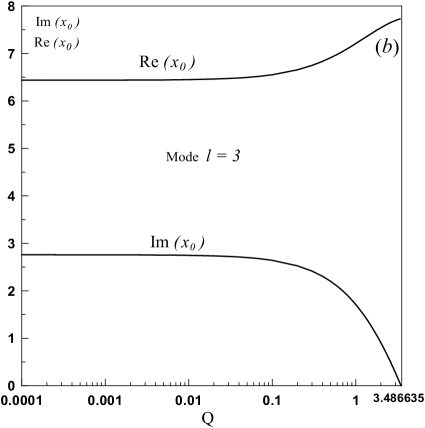
When the supercriticality of $\delta Q$ is not small, the perturbation theory above does not allow us to calculate the complex eigenfrequency. In this case, the characteristic equation (4.31) was solved numerically, for values of $n=2,\ldots,5$. The qualitative behavior of real and imaginary parts of the frequency is similar for all calculated cases. So we restrict our illustrations only to the model with $n=3$ (see Fig. 9). Note also that the results of computations, for small deviations from the stability boundary, coincide with the asymptotic results obtained using the perturbation theory (4.35).

Figure 9: Loss-cone instability in spherical system. a – DF over precession angular velocity ${\bar{f}}_{n=3}=x^{3}\,\exp(-x)$. The dash lines indicate positions of resonances for neutral mode. (Squared dimensionless frequency is $x_{0}=7.733736$.); b – Behavior of squared dimensionless frequency $x_{0}$ of unstable mode. The values of ${\rm Re}\,(x_{0})$ and ${\rm Im}\,(x_{0})$ are shown against parameter ${\bar{Q}}$.

4.8 General instability criterion and study of specific distributions

The above results, based on the neutral mode approach, can also be obtained using a suitable analogue by means of the well-known Penrose – Nyquist theorem (Penrose 1960, Mikhailovsky 1974). Recall that this theorem is widely used in plasma physics. Employing the theorem helped to establish numerous general results in the theory of plasma instabilities.

First we represent our characteristic equation in the form

$${Q}=C_{l}\int\limits_{0}^{\infty}dx\,x\,\frac{d\,{f}(x)}{dx}\sum\limits_{s\,=\,s_{\rm min}}^{l}\frac{D_{l}^{s}}{x-z/s^{2}},$$ (4.37)

where the quantity $Q$ is independent of $l$. In the case of retrograde precession we are interested in, $Q>0$. Recall that $s_{\rm min}$ is equal to 1 or 2 depending on evenness of $l$, $x=\nu^{2}$ is the precession angular velocity squared, in dimensionless units (the units of $\nu_{T}$, where $\nu_{T}$ is the precession velocity dispersion, is common), $f(x)$ is the unperturbed DF, $z=\omega^{2}$ is the frequency squared, in the same dimensionless units.

We are also reminded that the singularity of the integral in the right side of (4.37), for $z$ on the real axis, must be bypassed from below if ${\rm Re}\,(\omega)>0$, and above if ${\rm Re}\,(\omega)<0$. From this indentation rule and the form of Eq. (4.37), it immediately follows that complex unstable roots, $z_{0}$, form pairs: if $z=z_{0}=a+i\,b,\ \ a\neq 0,\ \ b>0$ – the root of Eq. (4.37), and the corresponding eigenfrequency is $\omega=\omega_{0}=\alpha+i\,\beta$, ($\alpha>0,\ \ \beta>0$), the complex conjugate root, $z={\bar{z}}_{0}=a-i\,b$, also satisfies Eq. (4.37) and describes the mode with the same growth rate, but opposite sign of frequency, $\omega=-{\bar{\omega}}_{0}=-\alpha+i\,\beta$.

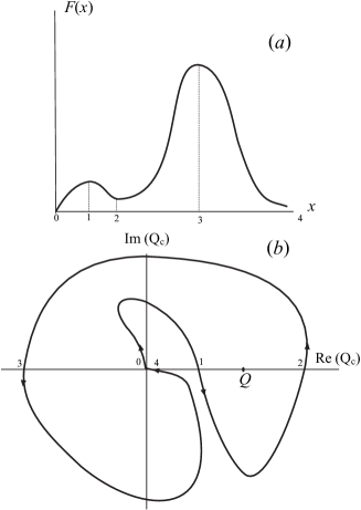
Note that the form of Eq. (4.37) shows that the aperiodic instability, for which ${\rm Re}\,(z_{0})<0,\ {\rm Im}\,(z_{0})=0$, i.e., $a=0$, is absent here. Indeed, putting $z_{0}=-|z_{0}|<0$ in (4.37) and integrating by parts, it is easy to verify that the right side of (4.37) is negative. By the way, this is a further distinction of Eq. (4.37) from the disk characteristic equation that allows aperiodic instabilities for symmetric distributions $f(\nu)$.

Eq. (4.37) involving $[\frac{1}{2}\,(l+1)]$ items can be reduced to a one-term equation. Indeed, the substitution

$$F^{(l)}(x)=C_{l}\sum\limits_{s\,=\,s_{\rm min}}^{l}{D_{l}^{s}}\,f\bigl{(}{x}/{s^{2}}\bigr{)}.$$ (4.38)

transforms (4.37) into the equation

$${Q}=\int\limits_{0}^{\infty}dx\,x\,\frac{d\,{F}^{(l)}(x)/dx}{x-z}.$$ (4.39)

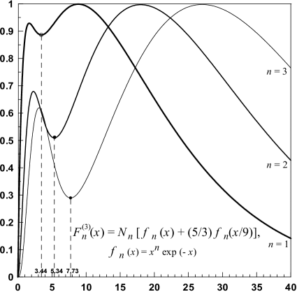
Thus, for arbitrary values of $l$, we obtain a one-item equation (4.39) similar to that for the mode $l=2$ (or $l=1$). However, now the integral involves the function $F^{(l)}(x)$, instead of the initial function $f(x)$ (with one maximum and tending to zero at $x=0$ and infinity). Starting with modes $l=3$, the new function, $F^{(l)}(x)$, can have minima. It is easy to understand that the frequencies (candidates for a neutral mode) calculated in subsection 4.6 from the condition of balance between growth and damping at resonances on different sides of the maximum of the initial function $f(x)$, are precisely those coinciding with the extrema of the new function, $F^{(l)}(x)$, i.e., $z=x_{j}$, $F^{\prime}(x_{j})=0$. Correlating this with earlier results for disks, and also with the sphere DF $f_{n}(x)=x^{n}\exp\,(-x)$, we become convinced that the largest (more often, the only) positive critical value of $Q_{c}$ for the neutral mode should necessarily be related to a minimum of the DF $F^{(l)}(x)$. As an illustration of this statement, Fig. 10 shows three functions $F^{(l)}_{n}(x)$ of this series, for the mode $l=3$. From the figure (and also Table 2), it is seen that only the central of these three extrema, i.e., the minimum, gives rise to the neutral mode with positive values of $Q_{c}$ (for $n\geq 1$).

Figure 10: – Function $F_{n}^{(l)}(x)$ for a model $f(x)=x^{n}e^{-x}$ with $l=3$ ($n=1,\,2$ and 3).

Thus, we see that the availability of minima is of fundamental importance for the existence of neutral modes with positive $Q_{c}$ (and consequently for instability). We have already seen that for $l=1$ and $l=2$, when the DF $F^{(l)}(x)$ coincides with the initial DF $f(x)$, so that the former has no minima, the corresponding neutral modes (and instability) are absent.

Recall that the possible-in-principle neutral mode with $z=0$ corresponding to the resonance at the minimum $x=0$, has $Q_{c}=0$, so that it cannot be assumed to be a candidate for a neutral mode with the property required for instability ($Q_{c}>0$). Therein lies a fundamental difference from disks where any two-hump distribution with a zero minimum at $\nu=0$ always has the neutral mode with $Q_{c}>0$ at the minimum. So such a distribution is always unstable (when $Q<Q_{c}$) independently of other DF details.

We have a right to expect a neutral mode (and instability) related to the minimum, for $l\geq 3$ only. In fact, it has already been demonstrated above using a somewhat more cumbersome method. Besides, a question remains unsolved in the approach we apply: why are not all distributions with one maximum that vanishes at the ends of the positive semi-axis $0\leq x<\infty$ generally unstable, even though $l\geq 3$. Empirically, by considering various series of distribution functions, we found the qualitative instability condition. Its rough formulation is: the instability is possible if the DF function is well-localized around its maximum.

Now a possibility appears for a more rigorous (in fact, quantitative) formulation of the instability condition. Though Eq. (4.39) differs from the equation

$${Q}=\int\limits_{-\infty}^{\infty}\frac{f^{\prime}(v)\,dv}{v-c},$$ (4.40)

(where $c=\omega/k$ is the complex phase velocity, $Q=k^{2}/\omega_{0}^{2}>0$, $k$ is the wave number, $\omega_{0}^{2}=4\pi n_{0}e^{2}/m$ is the plasma frequency squared), for which Penrose (1960) obtained his well-known criterion, here we also can obtain an analogous criterion – i.e. a counterpart of the Penrose – Nyquist criterion, for our equation (4.39). First we formulate it in terms of neutral modes.

Theorem. The distribution $F^{(l)}(x)$ is stable if neutral modes corresponding to minima of $F^{(l)}(x)$ are absent. Alternatively, if at least one neutral mode corresponding to a minimum occurs, then a sufficiently small $Q$ always exists, for which the system will be unstable relative to perturbations with a given $l$.

The instability condition for any $l$ follows immediately from the theorem. Indeed, if for at least one of $l$ ($l=1,2,\ldots$), a neutral mode exists for the corresponding distribution $F^{(l)}(x)$, then such a sufficiently small $Q$ occurs, for which the system is unstable.

It is useful to give another formulation of the theorem with a maximally possible similarity to that of Penrose (1960) for Eq. (4.40).

Theorem (another formulation). The distribution $F^{(l)}(x)$ is stable if and only if for all points $x_{j}$, at which the modified DF $F^{(l)}(x)$ has a minimum (i.e., $F^{\prime}(x_{j})=0,\ \ F^{\prime\prime}(x_{j}>0$), the condition

$${Q_{c}}\equiv\int\limits_{0}^{\infty}dx\,x\,\frac{d\,{F}^{(l)}(x)/dx}{x-x_{j}}<0.$$ (4.41)

is met. Conversely, if at least for one minimum the opposite inequality is satisfied, then such a sufficiently small $Q$ exists, for which the system is unstable for perturbations with a given $l$.

The proof of this theorem can be found in Appendix B, but now we discuss a correlation between the instability condition following from this criterion and our qualitative condition formulated above.

From the results obtained for disks, we know that under sufficiently deep minimum, the corresponding $Q_{c}$ can become positive. Thus, it can rigorously be shown that $Q_{c}>0$ (with a finite margin) in the limit when the minimum is exactly equal to zero.

Indeed, let us assume that $x_{j}$ is the position of minimum, at which $F(x_{j})=0$, $F^{\prime}(x_{j})=0$. Then we obtain by integrating in (4.41) by parts

$${Q_{c}}\equiv\int\limits_{0}^{\infty}dx\,x\,\frac{d\,{F}^{(l)}(x)/dx}{x-x_{j}}=x_{j}\int\limits_{0}^{\infty}dx\,\frac{d\,{F}^{(l)}(x)/dx}{x-x_{j}}=$$

$$=x_{j}\int\limits_{0}^{\infty}dx\,\frac{{F}^{(l)}(x)}{(x-x_{j})^{2}}>0.$$

It becomes impossible to prove in a similar manner that the integral is also positive for a non-zero minimum. Actually, it can have any sign. However, positive contributions into the integral increase the closer the minimum is to zero. So the integral should eventually become positive with increasing depth of minimum.

In light of this fact, it becomes clear that our qualitative instability condition means that a minimum of $F^{(l)}(x)$ is sufficiently deep, so that the related neutral mode occurs. This becomes evident when we consider how the function $F^{(l)}(x)$ is built from the initial DF $f(x)$. The instability is unavailable if a minimum is absent or is not sufficiently deep. In Fig. 10, the functions $F_{n}^{(l)}(x)$ constructed from the functions $f_{n}(x)=x^{n}\,e^{-x}$, for the mode $l=3$, are for convenience calibrated so that the value of the highest maximum is equal to unity for all values of $n$. We see that the only minimum becomes deeper with increasing $n$. This is in complete agreement with the results of Sec. 4.7 where we found that the mode $l=3$ is stable for $n=1$ and unstable for $n\geq 2$. (For completeness we additionally checked that instability emerges when $n>1.55$). Moreover, we checked that the instability in the model with $n=1$ is also absent for any $l$.

The formulated criterion allows a purposeful search for such DF $f(x)$ which gives a new function $F(x)$ with a minimum capable of ‘generating” a neutral mode. In other words, the integral (4.41),

$$Q_{c}=\int\limits_{0}^{\infty}dx\,x\,\frac{d\,{F}^{(l)}(x)/dx}{x-x_{j}}\equiv x_{j}\int\limits_{0}^{\infty}dx\,\frac{F^{(l)}(x)-F^{(l)}(x_{j})}{(x-x_{j})^{2}},$$ (4.42)

is positive, so that the instability occurs when $Q<Q_{c}$. It turns out that suitable distributions are known in plasma physics. In particular, Penrose (1960) has pointed to a case of such a distribution. Namely, he demonstrated that a plasma distribution becomes unstable provided this distribution has a sufficiently sharp minimum (then the Penrose integral similar to (4.42) becomes positive). For instance, such a minimum appears at the electron DF when a sufficiently cool electron beam is injected into the Maxwellian plasma, provided the beam velocity is larger than the electron thermal velocity of main plasma.

It is interesting that distributions with sharp minima appear in our problem quite naturally. Indeed, let us assume that the star distribution with respect to angular momenta (or, which is the same, to precession angular velocities) is Gaussian. In terms of the variable $x=\nu^{2}/\nu_{T}^{2}$, it has the form $f(x)=N\,e^{-x}$, $0<x<\infty$, $N$ is the normalized constant. Now we suggest that the stars enclosed by the loss cone elude the distribution so that the resulting distribution arises:

$$f(x)=N\,H(x-a)\,e^{-x},$$ (4.43)

where $H(t)$ is the Heaviside step function. Any physically admissible distribution should of course be smooth. So, instead of discontinuous function (4.43), we assume a nearly identical (but continuous and smooth) distribution

$$f(x)=N\,{\cal R}_{a}(x)\,e^{-x},\\ {\cal R}_{a}(x)={\textstyle\frac{1}{2}}\left[\tanh\,\Bigl{(}\frac{x-a}{\delta}\Bigr{)}+\tanh\,\Bigl{(}\frac{a}{\delta}\Bigr{)}\right],$$ (4.44)

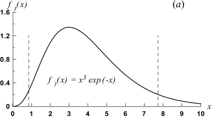
where $\delta\ll a$ in the “cutting factor” ${\cal R}_{a}(x)$. The function

$$F(x,a)=\frac{1}{16}\,C_{3}\,\bigl{[}3\,f(x)+{5}\,f(\textstyle\frac{1}{9}\,x)\bigr{]}$$

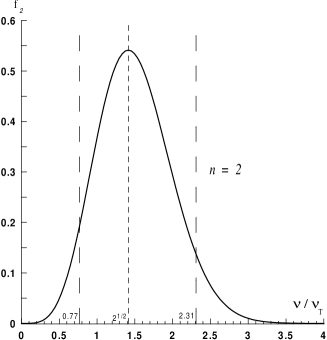
for the mode $l=3$, corresponding to the DF (4.44) with $a=0.1$, $a=0.01$ and $\delta=\frac{1}{20}\,a$, is shown in Fig. 11 (a). It is seen that the distribution $F(x)$ has only one minimum, this minimum being sufficiently sharp. Direct calculations show that the neutral mode ($Q_{c}>0$) corresponding to the minimum occurs under an arbitrarily small size of a “slot” (i.e., a value of $a$). Fig. 11 (b) shows the marginal curve on the plane $(Q-a)$, where the modes with arbitrary values of $l$ are taken into account. It is seen that for not too large values of $a$ the boundary of instability is nevertheless actually determined by the first unstable mode $l=3$ only.

Figure 11: (a) – Function $F(x,a)=\frac{1}{16}\,C_{3}\,[3\,f(x)+5\,f(\frac{1}{9}\,x)]$ for the model (8) with $l=3$ and $a=0.01$, $a=0.1$ ($\delta=a/20$). (b)– the marginal curve on the $(Q-a)$ – plane, calculated for all $l$.

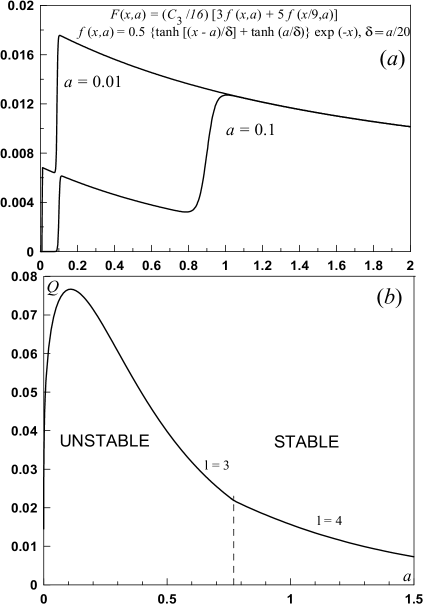
Thus, we see that an empty loss cone, even if it is very narrow, inevitably leads to the instability, for suitable distributions (i.e., the dispersion $\nu_{T}$ is less than the critical value $(\nu_{T})_{c}$ determined by the parameter $Q_{c}$.)

5 Discussion

First we list the results of the paper.

1. The paper presents a systematic derivation, from general linearized Vlasov equations (written in the action-angle variables), of simple characteristic equations for small perturbations in disk and spherical stellar systems with near-radial orbits.

2. On the one hand, our analysis of these characteristic equations confirms the presence (already discussed earlier, Polyachenko 1991b, Tremaine 2005) of gravitational loss-cone instability in disks. On the other hand, we succeeded to prove, in this paper, a possibility of this instability in spherical clusters.

3. It is shown that the physical reason of the instability under consideration is escape of stars through the loss cone due to destruction of stars with sufficiently low angular momenta. As a result, the DF in angular momenta will assume an unstable (“beam-like”) form. This is very similar to the situation in plasma traps (mirror machines) where plasma particles with low transversal (relative to the axis of the trap) velocities escape those systems. For this reason, distribution over these transversal velocities also becomes “beam-like”, so that the classical loss-cone instability develops.

4. We highlight retrograde precession of orbits as a necessary condition for the gravitational loss-cone instability. Expressions for precession velocity both in non-singular and near-Keplerian potentials are derived. In particular, they helped to obtain conditions for the the precession to become retrograde.

5. While deriving the characteristic equations, we justify the obvious (and very convenient for practical use) rotating-spokes approximation.

6. For analyzing the characteristic equations, a specific method is developed. It is based on preliminary search of neutral modes.

7. We also developed a method based on generalization of the plasma (and, in fact, gravitating disk) Penrose – Nyquist theorem that establishes the criterion of stability and instability. First, from an initial DF of stars in a spherical cluster, $f$, we turn to another, effective DF, $F$. The latter is constructed from $f$ according to a simple recipe (see the beginning of Subsec. 4.8). Using this new function, the many-term characteristic equation describing perturbations in spherical systems reduces to the simplest one-term disk-like equation. In turn this allows us to formulate and prove the above-mentioned generalization of the Penrose – Nyquist criterion.

8. It is shown that this criterion allows us to justify the following qualitative criterion of the gravitational loss-cone instability: the instability is possible if the DF is well-localized about its maximum. Using the criterion, we can perform a purposeful search of unstable distributions. In particular, we succeeded in proving an empty loss cone, even if very narrow, to be able to lead to instability.

Let us remind that for spherical near-Keplerian systems, Tremaine does not find the instability, although his integral equation (55) is equivalent to our “slow” equation (4.8), and the problem definition is very similar to ours: To study the stability of spherical models against comparatively slow perturbations (with typical times of the order of inverse precession frequency) provided that DF possesses positive derivative $\partial F/\partial L>0$ at low angular momentum due to the loss-cone.

Still, there are two considerable differences. The first one is that Tremaine (2005) has used Goodman’s (1988) criterion, which is fundamentally restricted to the modes $l\leq 2$. The second one is that Tremaine studied only monotone DF (from radial orbits $L=0$ up to circular orbits $L=L_{\rm circ}$). In that case the variational principle takes place, which claims that squares of eigen frequencies should be real (${\rm Im}(\omega^{2})=0$). So the unstable modes are aperiodic, if any. Tremaine (2005) has shown that for the models considered ($\log$-models, see (98) in his paper), stabilizing and destabilizing contributions cancel each other for $l=1$ leading to neutrally stable lopsided mode $\omega^{2}=0$, while for $l=2$ the stabilizing contribution dominates.

In our case non-monotone DFs violate the variational principle, so that the squares of eigen frequencies should not be real. Moreover, we have shown (Sect. 4.8) that the aperiodic instability is impossible, i.e. the eigenmodes are oscillating, ${\rm Re}(\omega)\neq 0$. We have found the instability at $l\geq 3$ for spherical models, if DFs have maximum somewhere in the region $0<L<L_{\rm circ}$. It is plausible that we deal with instabilities of somewhat different nature.

By considering two-humped models in Sect. 3, we demonstrated that the gravitational loss-cone instability can arise in disks with nearly radial orbits. One can show that two-humped DFs is crucial for the instability. Such distributions arise naturally from originally Maxwell-like DFs after consumption of stars with low angular momenta by a black hole. The instability takes place for arbitrary azimuthal number $m$. Meanwhile Tremaine (2005) has considered distributions in the interval $-L_{\rm circ}<L<L_{\rm circ}$, which is symmetric around $L=0$. On the example of lopsided mode $l=1$, he has shown that disk is generally unstable. Note that condition (3.11) is implicitly suggested in his derivation of instability criterion (Eq. (114) in Tremaine (2005)).

For the final conclusion on which of two differences is decisive for the instability, i.e. monotonity or mode number $l\geq 3$, some additional work is needed. We hope to attack this problem in future using our “slow” equation, derived in Sect. 4. The problem seems to be of importance since in some numerical models (e.g., Cohn and Kulsrud, 1978) collisions result in the establishment of distributions growing monotonically (from the loss-cone boundary up to circular orbits). It is likely that such distributions will prove to be stable (see recent N-body experiments by Berczik et al. (2005)). On the other hand, we also emphasize the fact that such a “near-isotropy” observed in some numerical simulations is not an unambiguously established fact at present. Not to mention that distributions with prevalent elongated orbits can be quite natural in some circumstances (e.g., periods between their formations due to, say, collisionless collapse, and the moment of relaxation).

In the paper by Berczik et al. (2005) N-body simulations have been used to model the loss cone in the vicinity of the (binary) black hole. The model allowed them to construct the lose cone which was maintained in nearly-empty state during simulations. However the black hole feeding rate was at the level consistent with standard collisionally-repopulated loss-cone theory. The discrepancy between their and our results is probably explained by difference in character of distribution over angular momentum. Berczik et al. (2005) have assumed initially homogeneous system, which leads to the near-isotropic one in the course of collision evolution (more exactly, to the distribution slightly growing with $L$ if to ignore a small region of empty loss-cone), whereas we have proved instability for systems with nearly radial orbits. Yet, this N-body modelling can be a weighty argument in favour of stability of monotone distribution functions.

In conclusion we present preliminary estimations of efficiency of the collective mechanism under consideration. For the most interesting, near-Keplerian, case, such estimates were made by Tremaine (2005), and we use these estimates below.

There are several characteristic time scales. The first is the dynamical time, $t_{\rm dyn}\sim\Omega^{-1}\sim(R^{3}/GM_{c})^{1/2}$, where $R$ is the typical orbital radius, $M_{c}$ is the central point mass. The orbit precession determines, using Tremaine’s (2005) terminology, the secular time scale,

$$t_{\rm sec}\sim t_{\rm dyn}\frac{M_{c}}{M_{G}}\sim t_{\rm dyn}\frac{M_{c}}{N_{G}m},$$

where $M_{G}$, $N_{G}$ and $m$ is the cluster mass, the number of stars and the mass of one star, respectively. The gravitational loss-cone instability develops precisely on this time scale (cf. the formula (4.15) for the precession velocity in our monoenergetic model, $\gamma={\rm Im}\,(\omega)\sim\Omega_{\rm pr}=\varpi L\sim({M_{G}}/{M_{c}})\,({L}/{R^{2}})\sim\Omega\,({M_{G}}/{M_{c}})$.) The next important time scale defines a period of collision relaxation,

$$t_{\rm relax}\sim\frac{R^{3/2}M_{c}^{3/2}}{G^{1/2}m\,M_{G}}\sim t_{\rm dyn}\frac{M_{c}^{2}}{m\,M_{G}}\sim t_{\rm dyn}\frac{M_{c}^{2}}{m^{2}\,N_{G}}.$$

These three time scales are well-known. Tremaine (2005) introduces another (less known) time scale, citing his paper (Rauch & Tremain, 1996) – the time of resonance relaxation of angular momenta,

$$t_{\rm res}\sim\frac{R^{3/2}M_{c}^{1/2}}{G^{1/2}m}\sim t_{\rm dyn}\frac{M_{c}}{m}.$$

For near-Keplerian systems (when $M_{G}\ll M_{c}$, $N_{G}\gg 1$), these four time scales are highly separated:

$$t_{\rm dyn}\ll t_{\rm sec}\ll t_{\rm res}\ll t_{\rm relax}.$$

Thus, according to these estimates by Tremaine, the instability should grow faster than collisional (and resonant) relaxation, whether or not a cluster mass is small.

Note, however, that the estimates of time scales presented here are insufficient to claim that the collective mechanisms under consideration should dominate. There is a need to calculate and compare the star fluxes onto the black hole. In this connection, we should remind the reader that so far we only attempted to prove that the instability is possible in principle.

APPENDIX A. Derivation of the integral equation for perturbations in a spherically-symmetric gravitating system in terms of the action-angle formalism

1. The action-angle variables in a spherically-symmetric potential

Let us recall the action-angle variables in a spherically-symmetric potential $\Phi_{0}(r)$.

The action variables:

$$I_{1}=\frac{1}{2\pi}\oint p_{r}dr=\frac{1}{\pi}\int\limits_{r_{\rm min}}^{r_{\rm max}}\sqrt{2E-2\Phi_{0}(r)-L^{2}/r^{2}}dr,$$

$$I_{2}=\frac{1}{2\pi}\oint p_{\theta}d\theta=\frac{1}{\pi}\int\limits_{\theta_{0}}^{\pi-\theta_{0}}d\theta\,\sqrt{L^{2}-L_{z}^{2}/\sin^{2}\theta}=L-|L_{z}|,$$

$$I_{3}=\frac{1}{2\pi}\oint p_{\varphi}\,d\varphi=L_{z}.$$

Here $E=\frac{1}{2}\,{v_{r}^{2}}+\frac{1}{2}\,{L^{2}}/{r^{2}}+\Phi_{0}(r)$ is the particle energy, $L=r\sqrt{v_{\theta}^{2}+v_{\varphi}^{2}}=\sqrt{p_{\theta}^{2}+{p_{\varphi}^{2}}/{\sin^{2}\theta}\phantom{\big{|}}}$ is its angular momentum magnitude, and $L_{z}=r\,\sin\theta\,v_{\varphi}$ is a projection of the angular momentum on the axis $z$. The angle $\theta_{0}$ is defined as $\sin^{2}\theta_{0}={L_{z}^{2}}/{L^{2}},$ and the generalized impulses are defined as follows $p_{r}=\dot{r}=v_{r},\ \ p_{\theta}=r^{2}\,\dot{\theta}=r\,v_{\theta},\ \ p_{\varphi}=r^{2}\sin^{2}\theta\,\dot{\varphi}=r\sin\theta\,v_{\varphi}.$ Note that it follows from (A2) and (A3) that $L=I_{2}+|I_{3}|,\ \ L_{z}=I_{3}.$

The angular variables.

By definition angular variables $w_{1},\ w_{2},\ w_{3}$ are $w_{i}={\partial S}/{\partial I_{i}}.$ The function of action $S$ in a spherically-symmetric potential is known to allow for separating the variables and can be written as a sum $S({\mbox{\boldmath$I$}};r,\theta,\varphi)=S_{1}+S_{2}+S_{3},$ where the components $S_{1}$, $S_{2}$ and $S_{3}$ are

$$S_{1}=\int\limits_{r_{\rm min}}^{r}dr^{\prime}\sqrt{2E\,({\mbox{\boldmath$I$}})-2\Phi_{0}(r^{\prime})-{(I_{2}+|I_{3}|)^{2}}/{r^{\prime\,2}\phantom{\big{|}}}},$$

$$S_{2}=\int_{\theta_{0}}^{\theta}p_{\theta}\,d\,\theta^{\prime}=\int\limits_{\theta_{0}}^{\theta}\sqrt{(I_{2}+|I_{3}|)^{2}-{I_{3}^{2}}/{\sin^{2}\theta^{\prime}}\phantom{\big{|}}}\,d\theta^{\prime},$$

$$S_{3}=\int\limits_{0}^{\varphi}I_{3}\,d\varphi^{\prime}=I_{3}\,\varphi.$$

For convenience, we accepted a symbolical, “vector”, designation ${\mbox{\boldmath$I$}}=(I_{1},I_{2},I_{3})$. We have

$$w_{1}={\partial S}/{\partial I_{1}}={\partial S_{1}}/{\partial I_{1}}=\Omega_{1}\int\limits_{r_{\rm min}}^{r}\frac{dr^{\prime}}{\sqrt{2E-2\Phi_{0}(r^{\prime})-{L^{2}}/{r^{\prime\,2}}\phantom{\big{|}}}},$$

$$w_{2}={\partial S_{1}}/{\partial I_{2}}+\int\limits_{\theta_{0}}^{\theta}d\,\theta^{\prime}\frac{I_{2}+|I_{3}|}{\sqrt{(I_{2}+|I_{3}|)^{2}-{I_{3}^{2}}/{\sin^{2}\theta^{\prime}}}}$$

$$={\partial S_{1}}/{\partial I_{2}}+\arccos\left(\frac{\cos\theta}{\cos\theta_{0}}\right),$$

$$w_{3}={\partial S_{1}}/{\partial I_{3}}+{\partial S_{2}}/{\partial I_{3}}+\varphi.$$

Action variables are integrals of motion, and angular variables linearly depend on time: $w_{i}(t)=w_{i}(0)+\Omega_{i}({\mbox{\boldmath$I$}})\,t$, where frequencies $\Omega_{j}({\mbox{\boldmath$I$}})$ are $\Omega_{j}={\partial E(I_{1},I_{2},I_{3})}/{\partial I_{j}}$.

2. The solution of the kinetic equation, calculation of perturbed density and derivation of the integral equation

The perturbation of the DF $f_{1}$ is easily obtained from the kinetic equation if we write it down in terms of action-angle variables:

$$\frac{df_{1}}{dt}\equiv\frac{\partial f_{1}}{\partial t}+\Omega_{i}\,\frac{\partial f_{1}}{\partial w_{i}}=\frac{\partial F}{\partial I_{i}}\,\frac{\partial\Phi}{\partial w_{i}}.$$

We have

$$f_{1}=-\frac{1}{(2\pi)^{3}}\sum\limits_{l_{1},\,l_{2},\,l_{3}}\Phi_{l_{1},\,l_{2},\,l_{3}}({\mbox{\boldmath$I$}})\,\frac{l_{j}\,{\partial F}/{\partial I_{j}}}{\omega-l_{j}\,\Omega_{j}}\,e^{i\,(l_{j}\,w_{j}-\omega\,t)},$$

This involves summation over a repeating index $j=1,\,2,\,3$. In what follows the background DF $F$ is supposed to be dependent on $E$ and $L$ only. The function $\Phi_{l_{1},\,l_{2},\,l_{3}}({\mbox{\boldmath$I$}})$ appearing in (A4) is

$$\Phi_{l_{1},\,l_{2},\,l_{3}}({\mbox{\boldmath$I$}})=\int\limits_{0}^{2\pi}dw_{1}\int\limits_{0}^{2\pi}dw_{2}\int\limits_{0}^{2\pi}dw_{3}\,\,\Phi({\mbox{\boldmath$I$}},{\mbox{\boldmath$w$}})\,\exp\,(i\,{\mbox{\boldmath$l$}}\,{\mbox{\boldmath$w$}}),$$

where another symbolical “vector” designation are introduced for brevity: ${\mbox{\boldmath$w$}}=(w_{1},w_{2},w_{3})$ and ${\mbox{\boldmath$l$}}=(l_{1},l_{2},l_{3})$. In Eq. (A5) the function $\Phi({\mbox{\boldmath$I$}},{\mbox{\boldmath$w$}})$ represents the perturbation of potential (without the factor $e^{-i\omega t}$) expressed in variables $({\mbox{\boldmath$I$}},{\mbox{\boldmath$w$}})$. We shall choose this function in the form

$$\Phi(r,\theta,\varphi)=\chi(r)\,P_{\,l}(\cos\theta),$$

where $P_{l}(x)$ is Legendre polynomial. In the main text we have already given arguments why we may confine ourselves to the case $m=0$, without considering perturbations with a more general angular structure of the type $Y_{l}^{m}(\theta,\varphi)=P_{l}^{m}(\cos\theta)\,e^{im\varphi}$, where $P_{l}^{m}(x)$ is the associated Legendre function. This results in certain simplifications, in particular, we may only deal with double, not triple, summation. We have $\Phi_{l_{1},\,l_{2},\,l_{3}=0}\equiv 2\pi\,\Phi_{l_{1},\,l_{2}},$ where, according to (A5),

$$\Phi_{l_{1},\,l_{2}}=\int\limits_{0}^{2\pi}dw_{1}\int\limits_{0}^{2\pi}dw_{2}\,\chi\,\bigl{[}r\,(I_{1},I_{2}+|I_{3}|),w_{1}\bigr{]}$$

$$\times\,P_{\,l}\biggl{[}\cos\theta_{0}\,\cos\Bigl{(}w_{2}-{\partial S_{1}}/{\partial I_{2}}\Bigr{)}\biggr{]}\,e^{-i\,(l_{1}\,w_{1}+l_{2}\,w_{2})},$$

and $\Phi({\mbox{\boldmath$I$}},w_{1},w_{2})=(2\pi)^{-2}\sum\Phi_{\,l_{1},\,l_{2}}({\mbox{\boldmath$I$}})\,e^{i\,(\,l_{1}\,w_{1}+l_{2}\,w_{2})}.$ The expression for perturbed DF also retains a mere double summation:

$$f_{1}\!=\!-\frac{1}{(2\pi)^{2}}\!\!\sum\limits_{l_{1},\,l_{2}}\!\Phi_{l_{1},\,l_{2}}({\mbox{\boldmath$I$}})\,\frac{l_{1}\,{\partial F}/{\partial I_{1}}\!+\!l_{2}\,{\partial F}/{\partial I_{2}}}{\omega-l_{1}\,\Omega_{1}-l_{2}\,\Omega_{2}}\,e^{i\,(l_{1}\,w_{1}+l_{2}\,w_{2})}.$$

Expression for $\Phi_{l_{1},\,l_{2}}({\mbox{\boldmath$I$}})$ can be transformed into a more compact form. For this purpose we shall first transform $P_{\,l}\bigl{[}\cos\theta_{0}\,\cos\bigl{(}w_{2}-{\partial S_{1}}/{\partial I_{2}}\bigr{)}\bigr{]}$, using the summation theorem for Legendre polynomials:

$$P_{\,l}(\cos\theta_{1}\cos\theta_{2}-\sin\theta_{1}\sin\theta_{2}\cos\varphi)$$

$$=\sum\limits_{k=-l}^{l}e^{-i\,k\,\varphi}P_{\,l}^{\,k}(\cos\theta_{1})\,P_{\,l}^{-k}(\cos\theta_{2}).$$

Substituting in this formula $\theta_{2}=\frac{1}{2}\,\pi,\ \ \ \theta_{1}=\frac{1}{2}\,\pi-\theta_{0},\ \ \varphi=w_{2}-{\partial S_{1}}/{\partial I_{2}}+\pi,$ let us write down

$$P_{\,l}\biggl{[}\cos\theta_{0}\,\cos\Bigl{(}w_{2}-{\partial S_{1}}/{\partial I_{2}}\Bigr{)}\biggr{]}=$$

$$=\sum_{k=-l}^{l}P_{\,l}^{\,k}(\sin\theta_{0})\,P_{\,l}^{-k}(0)e^{-ik\,\left(\,w_{2}-{\partial S_{1}}/{\partial I_{2}}\right)}e^{-ik\pi}$$

Substituting (A8) into (A7) and integrating over $w_{2}$, we obtain

$$\Phi_{l_{1},\,l_{2}}(E,L)=2\pi P_{\,l}^{\,l_{2}}(0)P_{\,l}^{-l_{2}}(\sin\theta_{0})e^{i\,l_{2}\pi}\chi_{l_{1},\,l_{2}}(E,L),$$

where

$$\chi_{l_{1},\,l_{2}}(E,L)=\int\limits_{0}^{2\pi}e^{-(l_{1}w_{1}+l_{2}\partial S_{1}/\partial I_{2})}\chi\,\bigl{[}r(E,L,w_{1})\bigr{]}\,dw_{1}.$$

For perturbed density $\rho(r,\theta,t)=\rho(r,\theta)\,e^{-i\omega t}$ we have

$$\rho(r,\theta)=\int f_{1}\,d{\mbox{\boldmath$v$}}=$$

$$=-\frac{1}{2\pi}\sum\limits_{l_{1},\,l_{2}}\int d{\mbox{\boldmath$v$}}\,P_{\,l}^{\,l_{2}}(0)P_{\,l}^{-l_{2}}(\sin\theta_{0})\,e^{i\,l_{2}\pi}\chi_{l_{1},\,l_{2}}(E,L)\,$$

$$\times\dfrac{l_{1}\,{\partial F}/{\partial I_{1}}+l_{2}\,{\partial F}/{\partial I_{2}}}{\omega-l_{1}\Omega_{1}-l_{2}\Omega_{2}}\,e^{i\,(\,l_{1}\,w_{1}+l_{2}\,w_{2})}.$$

To close the system, we shall use the integral version of the Poisson equation (which appears more convenient for our purposes than the Poisson equation itself)

$$\Phi(r,\theta)\!=-\,G\int\!\!\frac{\rho\,(r^{\prime},\theta^{\prime})\,dV^{\prime}}{\sqrt{r^{2}+r^{\prime\,2}-2\,rr^{\prime}\cos\Theta{\phantom{\big{|}}}}},$$

where $dV^{\prime}$ is a volume element and $\Theta$ is the angle between vectors $r$ and ${\mbox{\boldmath$r$}}^{\prime}$: $\cos\Theta=\cos\theta\cos\theta^{\prime}+\sin\theta\sin\theta^{\prime}\cos(\varphi-\varphi^{\prime})$. Using (A12) it is simple to obtain the integral connection between radial parts of perturbed density ${\hat{\rho}}(r)$ and potential $\chi(r)$. However, the simplest way of obtaining this connection is to directly solve, relative to $\chi(r)$, the known ordinary differential equation which follows from the Poisson equation after separating the angular dependence :

$$\frac{1}{r^{2}}\frac{d}{dr}\,\Bigl{[}r^{2}\,\frac{d\,\chi(r)}{dr}\Bigr{]}-\frac{l\,(l+1)}{r^{2}}\,\chi(r)=4\pi G\,{\hat{\rho}}(r).$$

Solving Eq. (A13) in terms of Green’s function, we shall find the required relation:

$$\chi(r)=-\frac{4\pi G}{2l+1}\int r^{\prime\,2}dr^{\prime}{\hat{\rho}}(r^{\prime})\,{\cal F}_{l}(r,r^{\prime}).$$

where

$${\cal F}_{l}(r,r^{\prime})=\frac{(r_{<})^{l}}{(r_{>})^{l+1}},\ \ r_{<}={\rm min}(r,r^{\prime}),\ \ r_{>}={\rm max}(r,r^{\prime}).$$

For obtaining the integral equation in the desired form it is necessary to write down (A14) in action-angle variables and to split it into harmonics $(l_{1},l_{2})$. For this purpose it is necessary to select a radial component ${\hat{\rho}}(r)$ from the general expression for density (A11) and then to substitute it into the r.h.s. of (A14). Further it is necessary to use relation (A10), connecting $\chi_{\,l_{1},\,l_{2}}(E,L)$ to $\chi(r)$, multiplying its both parts by $\exp{\bigl{[}-i\,(l_{1}\,w_{1}+l_{2}\partial S_{1}/\partial I_{2}\bigr{]}}$ and integrating over $w_{1}$. Let us execute the above described procedure. We have for ${\hat{\rho}}(r)$:

$${\hat{\rho}}(r^{\prime})=(l+{\textstyle\frac{1}{2}})\int\limits_{0}^{\pi}\rho(r^{\prime},\theta^{\prime})\,P_{\,l}(\cos\theta^{\prime})\,\sin\theta^{\prime}d\theta^{\prime}.$$

Using an explicit form of expression for density (A11) and substituting the function ${\hat{\rho}}(r^{\prime})$ found with the help of (A15) into r.h.s. of (A14), we obtain:

$$\chi(r)=G\sum\limits_{l_{1}^{\prime},\,l_{2}^{\prime}}\int d{\mbox{\boldmath$v$}}^{\prime}\int r^{\prime\,2}dr^{\prime}\int\limits_{0}^{\pi}\sin\theta^{\prime}d\theta^{\prime}P_{\,l}(\cos\theta^{\prime})\,{\cal F}_{l}(r,r^{\prime})$$

$$\times\,P_{\,l}^{l_{2}^{\prime}}(0)P_{\,l}^{-l_{2}^{\prime}}(\sin\theta_{0}^{\prime})\,e^{i\pi l_{2}^{\prime}}\chi_{\,l_{1}^{\prime}\,l_{2}^{\prime}}(E^{\prime},L^{\prime})\times$$

$$\times\frac{l_{1}^{\prime}\,{\partial F}/{\partial I_{1}^{\prime}}+l_{2}^{\prime}\,{\partial F}/{\partial I_{2}^{\prime}}}{\omega-l_{1}^{\prime}\,\Omega_{1}(E^{\prime},L^{\prime})-l_{2}^{\prime}\,\Omega_{2}(E^{\prime},L^{\prime})}\,e^{\,i(\,l_{1}^{\prime}w_{1}^{\prime}+l_{2}^{\prime}w_{2}^{\prime})}.$$

It is also possible to integrate explicitly over $w_{2}^{\prime}$ in (A16). For this purpose let us note that in r.h.s. of (A18) there is an integration over phase volume $\int d\Gamma^{\prime}=\int d{\mbox{\boldmath$v$}}^{\prime}dV^{\prime}$, which, obviously, may be represented as ${\displaystyle\int}d\Gamma^{\prime}=2\pi{\displaystyle\int}d{\mbox{\boldmath$I$}}^{\prime}dw_{1}^{\prime}\,dw_{2}^{\prime}$. Writing down again $P_{\,l}(\cos\theta^{\prime})$, similarly to (A8), as a series, we find

$$\int\limits_{0}^{2\pi}dw_{2}^{\prime}e^{\,il_{2}^{\prime}w_{2}^{\prime}}P_{\,l}(\cos\theta^{\prime})$$

$$=2\pi\,P_{\,l}^{\,l_{2}^{\prime}}(\sin\theta^{\prime})P_{\,l}^{-l_{2}^{\prime}}(0)\,e^{-il_{2}^{\prime}\pi}\,e^{\,i\,l_{2}\,\partial S_{1}/\partial I_{2}^{\prime}}.$$

As a result for $\chi(r)$ we obtain an expression which already retains only a single integration over angular variables, namely, over $w_{1}^{\prime}$:

$$\chi(r)=2\pi G\sum\limits_{l_{1}^{\prime},\,l_{2}^{\prime}}\int dI_{1}^{\prime}\,dI_{2}^{\prime}\,dI_{3}^{\prime}\Bigl{[}P_{\,l}^{l_{2}^{\prime}}(0)\,P_{\,l}^{-l_{2}^{\prime}}(\sin\theta_{0}^{\prime})\Bigr{]}\,$$

$$\times\left[P_{\,l}^{-l_{2}^{\prime}}(0)\,P_{\,l}^{l_{2}^{\prime}}(\sin\theta_{0}^{\prime})\right]\chi_{\,l_{1}^{\prime}\,l_{2}^{\prime}}(E^{\prime},L^{\prime})\,$$

$$\times\frac{l_{1}^{\prime}\,{\partial F}/{\partial I_{1}^{\prime}}+l_{2}^{\prime}\,{\partial F}/{\partial I_{2}^{\prime}}}{\omega-l_{1}^{\prime}\,\Omega_{1}(E^{\prime},L^{\prime})-l_{2}^{\prime}\,\Omega_{2}(E^{\prime},L^{\prime})}\,$$

$$\times\int\limits_{0}^{2\pi}dw_{1}^{\prime}\,{\cal F}_{l}\left[r,r^{\prime}(E^{\prime},L^{\prime};w_{1}^{\prime})\right]\,e^{\,i(\,l_{1}^{\prime}\,w_{1}^{\prime}+l_{2}^{\prime}\,\partial S_{1}/\partial I_{2}^{\prime})}.$$

Remembering that $F({\mbox{\boldmath$I$}})=F(E,L)$ does not depend on $L_{z}=I_{3}$ we can perform explicitly another integration, namely, over $\theta_{0}^{\prime}$. Taking it into account we find

$$\int\limits_{-\pi/2}^{\pi/2}P_{\,l}^{\,l_{2}^{\prime}}(\sin\theta_{0}^{\prime})P_{\,l}^{-l_{2}^{\prime}}(\sin\theta_{0}^{\prime})\,d\,(\sin\theta_{0}^{\prime})$$

$$=\int_{-1}^{1}dz\,\bigl{[}P_{\,l}^{\,l_{2}^{\prime}}(z)\bigr{]}^{2}\frac{(l-l_{2})!}{(l+l_{2})!}=\frac{2}{2l+1}.$$

Using a known relation for $P_{\,l}^{k}(0)$ we obtain for $\chi(r)$:

$$\chi(r)=\frac{4\pi G}{2l+1}\sum\limits_{l_{1}^{\prime}=-\infty}^{\infty}\sum\limits_{l_{2}^{\prime}=-l}^{l}D_{l}^{l_{2}^{\prime}}\int\frac{dE^{\prime}\,L\,dL^{\prime}}{\Omega_{1}(E^{\prime},L^{\prime})}\chi_{\,l_{1}^{\prime}\,l_{2}^{\prime}}(E^{\prime},L^{\prime})$$

$$\times\,\frac{\Bigl{[}\,l_{1}^{\prime}\,\Omega_{1}(E^{\prime},L^{\prime})+l_{2}^{\prime}\,\Omega_{2}(E^{\prime},L^{\prime})\Bigr{]}\,{\partial F}/{\partial E^{\prime}}+l_{2}^{\prime}\,{\partial F}/{\partial L^{\prime}}}{\omega-l_{1}^{\prime}\,\Omega_{1}(E^{\prime},L^{\prime})-l_{2}^{\prime}\,\Omega_{2}(E^{\prime},L^{\prime})}$$

$$\times\int\limits_{0}^{2\pi}dw_{1}^{\prime}\,{\cal F}_{l}\left[r,r^{\prime}(E^{\prime},L^{\prime};w_{1}^{\prime})\right]\,e^{\,i\,(\,l_{1}^{\prime}\,w_{1}^{\prime}+l_{2}^{\prime}\,\partial S_{1}/\partial I_{2}^{\prime})}.$$

The explicit expression for $D_{l}^{k}$ is presented in the main text (see (4.7)). Finally, we obtain the desired set of integral equations for $\chi_{\,l_{1},\,l_{2}}$ presented in the main text:

$$\chi_{\,l_{1},\,l_{2}}(E,L)=\frac{4\pi G}{2l+1}\sum\limits_{l_{1}^{\prime}=-\infty}^{\infty}\sum\limits_{l_{2}^{\prime}=-l}^{l}D_{l}^{l_{2}^{\prime}}\int\frac{dE^{\prime}\,LdL^{\prime}}{\Omega_{1}(E^{\prime},L^{\prime})}$$

$$\times\,\chi_{\,l_{1}^{\prime}\,l_{2}^{\prime}}(E^{\prime},L^{\prime})\,\Pi_{l_{1},\,l_{2};\,l_{1}^{\prime},\,l_{2}^{\prime}}(E,L;E^{\prime},L^{\prime})\times$$

$$\times\,\frac{\Bigl{[}\,l_{1}^{\prime}\,\Omega_{1}(E^{\prime},L^{\prime})+l_{2}^{\prime}\,\Omega_{2}(E^{\prime},L^{\prime})\Bigr{]}\,{\partial F}/{\partial E^{\prime}}+l_{2}^{\prime}\,{\partial F}/{\partial L^{\prime}}}{\omega-l_{1}^{\prime}\,\Omega_{1}(E^{\prime},L^{\prime})-l_{2}^{\prime}\,\Omega_{2}(E^{\prime},L^{\prime})},$$

where the kernel is

$$\Pi_{l_{1},\,l_{2};\,l_{1}^{\prime},\,l_{2}^{\prime}}(E,L;E^{\prime},L^{\prime})=$$

$$=\int\limits_{0}^{2\pi}dw_{1}\int\limits_{0}^{2\pi}dw_{1}^{\prime}\,{\cal F}_{l}\left[\,r\,(E,L;w_{1}),r^{\prime}(E^{\prime},L^{\prime};w_{1}^{\prime})\right]\times$$

$$\times\exp{\left\{\,i\,\left[\Bigl{(}\,l_{1}^{\prime}\,w_{1}^{\prime}+l_{2}^{\prime}\,{\partial S_{1}}/{\partial I_{2}^{\prime}}\Bigr{)}-\Bigl{(}l_{1}\,w_{1}+l_{2}\,{\partial S_{1}}/{\partial I_{2}}\Bigr{)}\right]\right\}}.$$

APPENDIX B. Instability criterion for the characteristic equation (4.39) – counterpart of Penrose - Nyquist plasma criterion

Let us write down the equation (4.39) in the form $\varepsilon^{(l)}(z,Q)=0$, where $\varepsilon^{(l)}(z,Q)\equiv 1-{Q_{c}(z)}/{Q}$ and complex function $Q_{c}(z)$ is defined as follows:

$$Q_{c}(z)=\int\limits_{0}^{\infty}dx\,x\,\frac{d\,{F}(x)/dx}{x-z}.$$

(Note that $Q_{c}(z)$ does not depend on $Q$.) In what follows the upper index $l$ is omitted for brevity. It is easy to understand that in the points of a real axis $z$, in which $z=z_{j}\equiv x_{j}$, where $x_{j}$ is any of the extremum points of the function $F(x)$, the function $Q_{c}(z)$ is real and coincides with the corresponding value $Q_{c}$ of the “neutral mode”. Quotation marks here are to reflect the fact that the corresponding value $z_{j}$ is not necessarily a squared frequency of a true neutral mode, since the sign of $Q_{c}(z_{j})$ can be any. Further we shall denote the real numbers $Q_{c}(z_{j})$ as $Q_{c}^{j}$ for brevity.

According to (B1) the function $Q_{c}(z)=Q_{c}(\omega^{2})$, considered as a function of $\omega$, is an analytic function in the $\omega$-plane cut along the real axis ${\rm Im}\,(\omega)=0$. From its definition (B1) it also follows that it is continuous and bounded (it tends to zero when $|\omega|\to\infty$). We are interested in unstable roots of the equations $\varepsilon(\omega^{2},Q)=0$, that is the roots lying in the upper half plane $\omega$. The number of such roots, according to the argument principle, coincides with the number of poles of the function $\varepsilon^{-1}$ in the upper half plane and is equal to $N=(2\pi i)^{-1}\int\limits_{C_{\omega}}d\omega\,{\varepsilon}^{-1}\,{d\varepsilon/d\omega}\,$ where the contour $C_{\omega}$ is shown on 12 (a). Turning to a variable $z=\omega^{2}$, we find

$$N=\frac{1}{2\pi i}\int\limits_{C_{z}}\frac{d\varepsilon/dz}{{\varepsilon}}\,dz,$$

where the directed contour $C_{z}$ is the image of a contour $C_{\omega}$ on a complex plane $z$. It is shown in Fig. 12 (b).

Figure 12: Directed contours of integration $C_{\omega}$ and $C_{z}$ on complex planes $\omega$ and $z$ respectively.

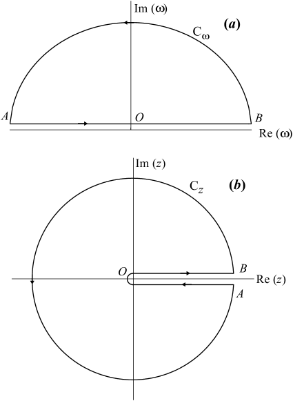
Following Penrose (1960), we shall pass from the complex plane $z$ to the complex plane $Q_{c}$. For the number of unstable roots $N$ we obtain the following expression

$$N=\frac{1}{2\pi i}\int\limits_{C_{z}}\frac{d\varepsilon/dz}{{\varepsilon}}\,dz=\frac{1}{2\pi i}\int\limits_{C_{{\varepsilon}}}\frac{d{\varepsilon}}{{\varepsilon}}=\frac{1}{2\pi i}\int\limits_{C_{Q_{c}}}\frac{dQ_{c}}{Q_{c}-Q},$$

where the directed contour $C_{Q_{c}}$ is the image of the directed contour $C_{z}$ on the complex plane $Q_{c}$.

Thus the problem is reduced to constructing a contour $C_{Q_{c}}$. The number of times that this contour encloses in anticlockwise sense the point $Q_{c}=Q$ (lying on the real positive half axis of the complex plane $Q_{c}$) will give us the number of unstable roots. We need to formulate rules according to which we should image a contour $C_{z}$ on the plane $Q_{c}$ and to establish a direction of motion along it in its various parts.

1. First of all, note that since the entire circle with a big radius on the plane $z$ is imaged into a unique point $Q_{c}=0$, the entire remaining contour $C_{Q_{c}}$ on the plane $Q_{c}$ corresponds to a horizontal part of the contour $C_{z}$, starting at a point $A$, and finishing at a point $B$.

2. It is easy to understand that the contour $C_{Q_{c}}$ is symmetric relative to the horizontal axis ${\rm Im}\,(Q_{c})=0$.

3. Further, we need to understand how the contour $C_{Q_{c}}$ crosses the horizontal axis at a point $Q_{c}=0$. Note that the contour $C_{Q_{c}}$ should cross the horizontal axis in this point (at least) twice. (i) The first crossing corresponds to the start of the contour from $Q_{c}=0$ and its finish at $Q_{c}=0$ when a point $z$ moves from $A$ to $B$ (that is the crossing corresponds to coincidence of the “initial” and “final” points of the closed contour. (ii) The second crossing corresponds to passage of a contour $C_{z}$ through a point $O$ (that is $z=0$). It follows directly from Equation (B1), that $Q_{c}(0)=0$. Let us examine the manner in which the contour $C_{Q_{c}}$ crosses the horizontal axis at $Q_{c}=0$ in both cases. The direction – up- or downwards – of the crossing of the real axis at this point is important here.

(i) We have from (B2) as $|z|\to\infty$

$$Q_{c}(z)=z\int\limits_{0}^{\infty}\frac{F^{\prime}(x)}{x-z}\,dx$$

$$=z\int\limits_{0}^{\infty}\frac{F(x)}{(x-z)^{2}}\,dx\approx\frac{1}{z}\int\limits_{0}^{\infty}F(x)\,dx=\frac{\cal M}{z},\ \ \ {\cal M}>0.$$

By means of (B3) it is now simple to understand that at a point $A$ (that is at $z=R-i\epsilon$, $R\to\infty,\ \ \epsilon\to 0$) ${\rm Im}\,(Q_{c})\to+0$, and at a point $B$ (that is at $z=R+i\epsilon$) ${\rm Im}\,(Q_{c})\to-0$. It means that this type of crossing is upwards. From (B3) it is also visible that crossing occurs so that ${\rm Re}\,(Q_{c})\to+0$, that is the contour approaches a point $Q_{c}=0$ from the right.

(ii) It is more difficult to establish how crossing occurs that corresponds to passage of a point $z=0$ on the contour $C_{z}$. Omitting details, we declare simply that crossing of the horizontal axis at a point $Q_{c}=0$ in this case also occurs upwards - however, the contour approaches this point so that ${\rm Re}\,(Q_{c})\to-0$, that is from the left.

4. Now we shall discuss the way the contour crosses the horizontal axis at points $Q_{c}^{j}$, corresponding to the extrema of $F(x)$. Clearly, each such point is crossed twice: the first crossing occurs when a point $z$ moves along the positive half axis from infinity to the center, and the second during subsequent movement in the opposite direction. We shall show that both crossings occur in the same direction, namely: downwards at points $Q_{c}^{j}$, corresponding to the maxima of $F(x)$, and upwards at points $Q_{c}^{j}$, corresponding to the minima. For points $z$ on the real axis $z$ we have

$$Q_{c}(z)=z\,\Bigl{[}\,\int\limits_{0}^{\infty}-\ dx\,\dfrac{F^{\prime}(x)}{x-z}+i\pi F^{\prime}(z)\,{\rm sign}\,(\omega)\Bigr{]},$$

so

$${\rm Im}\,[Q_{c}(z)]=\pi z\,F^{\prime}(z)\,{\rm sign}\,(\omega).$$

The origin of the factor ${\rm sign}\,(\omega)$ in (B4) and (B5) may be understood from Fig. 12 (b) where it is seen that for points $z$, lying a little below the positive half axis $z$, i.e., at ${\rm Im}\,(z)=-\epsilon$, the pole in the integral over $x$ in the right part (B2) is indented upwards, and for the points lying a little above the real axis, i.e., at ${\rm Im}\,(z)=\epsilon$, it is indented downwards.

Let the point $z$ pass through the corresponding extremum point $z_{j}$ during its first passage, that is from $A$ to $O$ along the bottom side of the positive real half axis. Then ${\rm sign}\,(\omega)=-1$, and the increment $\Delta z$ is negative, $\Delta z<0$. From (B5) we have

$$\Delta{\rm Im}\,[Q_{c}(z)]=\left\{\frac{d}{dz}\,{\rm Im}\,[Q_{c}(z)]\right\}_{z=z_{j}}\,\Delta z$$

$$=-\pi\,z_{j}\,F^{\prime\prime}(z_{j})\,\Delta z=\pi\,z_{j}\,F^{\prime\prime}(z_{j})\,|\Delta z|.$$

In its second crossing of this point, that is when the point $z$ moves from $O$ to $B$ along the top side of the positive real half axis, we have ${\rm sign}\,(\omega)=+1$ and $\Delta z>0$. So we again have

$$\Delta\,{\rm Im}\,[Q_{c}(z)]=\pi\,z_{j}\,F^{\prime\prime}(z_{j})\,\Delta z.$$

Thus, indeed, in both crossings the points $Q_{c}^{j}$, corresponding to extrema, pass in the same manner, namely, the minima ($F^{\prime\prime}(z_{j})>0$) upwards, and the maxima ($F^{\prime\prime}(z_{j})<0$) downwards.

The above recipes are sufficient to construct a directed contour $C_{Q_{c}}$. Having constructed it and found how many times it winds around the point $Q_{c}=Q$ lying on the horizontal axis to the right from the origin, we, according to Penrose’s idea, can draw a conclusion on the instability/stability of the system under consideration with a given value of the parameter $Q$. Indeed, from (B2) it is easy to understand that if the directed contour $C_{Q_{c}}$ crosses the horizontal axis from below to the right of the point $Q_{c}=Q>0$ at least once, then instability takes place ($N\geq 1$), since in this case the point $Q_{c}=Q$ is enclosed by the contour in an anticlockwise sense. As the parameter $Q$ can have an arbitrary positive value, we come to the conclusion that for instability it is necessary and sufficient that the contour crosses the horizontal positive half axis upwards at least once. It means that the rightmost crossing of the horizontal axis corresponds to a minimum of $F(x)$. This leads us to to formulating the instability criterion cited in subsection 4.8 of the main text.

Note that the task of constructing a contour can be simplified if we recall that it involves all unstable roots $z=z_{0}$ as complex conjugate pairs (this corresponds to pairs of eigenfrequencies $\omega_{0}=\pm\alpha+i\,\beta$, $\beta>0$). Therefore the number of times the contour $C_{Q_{c}}$ winds around a point $Q_{c}=Q$ in the complex plane $Q_{c}$ must be even, $N=2L$. It is simple to understand that $L$ times occur when a point $z$ moves in the complex plane $z$ from infinity to zero (along the bottom side of the real axis), and $L$ more times occur when it moves in the opposite direction (from $z=0$ to infinity along the top side). Recall that the full contour is symmetric relative to the horizontal axis, touches itself at point $Q_{c}=0$, and the horizontal axis is crossed twice at each point $z_{j}$ in the same direction - either both times downwards (maximum), or both times upwards (minimum). Therefore it is enough to trace the movement of point $z$ only halfway, say, from $z=0$ to infinity and to image only the half of the full contour which is also a closed contour. For definiteness we shall plot only that half which corresponds to movement of point $z$ from the center to infinity (along the top side of the real half axis). We shall designate this closed directed “semi-contour” as ${\hat{C}}_{Q_{c}}$ and, like the full contour, it will start and finish at point $Q_{c}=0$. Its beginning will be in the second quarter, and its end in the fourth quarter of the complex plane $Q_{c}$.

Note. The above does not mean that instability exists for any $0<Q<Q_{c}^{({\rm min})}$, where $Q_{c}^{({\rm min})}$ is a point of right-most crossing of a horizontal axis, related to a minimum $F(x)$. If a positive $Q_{c}^{({\rm max})}$ exists also for some maximum, instability will take place only when $Q_{c}^{({\rm max})}<Q<Q_{c}^{({\rm min})}.$ Indeed, from Fig. 13 it is seen that in this case the point $Q_{c}=Q$ will only be enclosed if $Q$ lies in the specified range.

Figure 13: Schematic sketch of DF $F(x)$ with two maxima and one minimum and corresponding arrangement of points $Q_{c}^{j}$ ($j=1,2,3$) on axis ${\rm Im}\,(Q_{c})=0$. Numbers 0, 1, 2, 3, 4 correspond to the order in which the directed semi-contour ${\hat{C}}_{Q_{c}}$ passes over corresponding points. The situation when there are two positive values $Q_{c}^{j}$ with $j=1$ and $j=2$, corresponding to low maximum, and to minimum, is demonstrated. The contour encloses a point $Q_{c}=Q$ in anticlockwise sense once provided that the point $Q$ is within the range $Q_{c}^{(1)}<Q<Q_{c}^{(2)}$. These values just are boundaries of the range of instability on parameter $Q$.

References

- Antonov (1973) Antonov V. A., 1973, Dynamics of galaxies and stellar clusters., Nauka, Alma-Ata, p. 139 (in Russian)
- Arnold (1989) Arnold V. I., 1989, Mathematical Methods of Classical Mechanics. Springer, Berlin
- Berczik et al. (2005) Berczik P., Merritt D., Spurzem R., 2005, ApJ, 633, 680
- Cohn & Kulsrud (1978) Cohn H., Kulsrud R. M., 1978, ApJ, 226, 1087
- Fridman & Polyachenko (1984) Fridman A. M., Polyachenko V. L., 1984, Physics of Gravitating Systems, Springer, New York
- Goodman (1988) Goodman J., 1988, ApJ, 329, 612
- Hickernell (1984) Hickernell F. J., 1984, J. Fluid Mech., 142, 431
- Landau & Lifshitz (1976) Landau L. D., Lifshitz E. M., 1976, Mechanics. Pergamon Press, Oxford
- Lightman, Shapiro (1977) Lightman A. P., Shapiro S. L., 1977, ApJ, 211, 244
- Lynden-Bell & Kalnajs (1972) Lynden-Bell D., Kalnajs A. J., 1972, MNRAS, 157, 1
- Lynden-Bell (1979) Lynden-Bell D., 1979, MNRAS, 187, 101
- Mikhailovsky (1974) Mikhailovsky A. B., 1974, Theory of plasma instabilities – I. Consultants Bureau, New York – London
- Penrose (1960) Penrose O., 1960, Phys. Fluids, 3, 258
- E. Polyachenko (2005) Polyachenko E. V., 2005, MNRAS, 357, 559
- E. Polyachenko (2004) Polyachenko E. V., 2004, MNRAS, 348, 345
- Polyachenko & Polyachenko (2004) Polyachenko V. L., Polyachenko E. V., 2004, Astronomy Report, 48, 877
- Polyachenko (1991a) Polyachenko V. L., 1991, Soviet Astron. Lett., 17, 292
- Polyachenko (1991b) Polyachenko V. L., 1991, Soviet Astron. Lett., 17, 371
- Polyachenko (1992) Polyachenko V. L., 1992, Sov. Phys. JETP, 74, 755
- Polyachenko & Shukhman (1972) Polyachenko V. L., Shukhman I. G., 1972, Preprint SibIZMIR, No. 1-2-72. Irkutsk (in Russian)
- Polyachenko & Shukhman (1980) Polyachenko V. L., Shukhman I. G., 1980, SvA, 24, 157
- Polyachenko & Shukhman (1981) Polyachenko V. L., Shukhman I. G., 1981, SvA, 25, 533
- Polyachenko & Shukhman (1982) Polyachenko V. L., Shukhman I. G., 1982, SvA, 26, 140
- Rauch & Tremain (1996) Rauch K. P., Tremaine S., 1996, New Astron., 1, 149
- Rosenbluth, Post (1965) Rosenbluth M. N., Post R. F., 1965, Phys. Fluids, 8, 547
- Shapiro, Marchant (1978) Shapiro S. L., Marchant A. B., 1978, ApJ, 225, 603
- Shukhman (1991) Shukhman I. G., 1991, J. Fluid Mech., 233, 587
- Sulentic & Keel (1990) Sulentic J. W., Keel W. C., 1990, in Sulentic J. W., Keel W. C., eds, Paried and Interacting Galaxies. IAY Colloq. No. 124, Tuscaloosa, Alabama 1989. NASA
- Tremaine (2005) Tremaine S., 2005, ApJ, 625, 143