Estimation of Galactic model parameters in high latitudes with 2MASS

Abstract

Context. In general, studies focused on the Milky Way’s structure show a range of values when deriving different Galactic parameters such as radial scalelengths, vertical scaleheights, or local space densities. Those values are also dependent on the Galactic coordinates under consideration for the corresponding analysis, as a direct consequence of be observing a structure (Our Galaxy), that is far from being as smooth and well-behaved as models usually consider.

Aims. In this paper, we try to find any dependence of the Galactic structural parameters with the Galactic longitude for either the thin disc or the thick disc of the Milky Way, that would indicate to possible inhomogeneities or asymmetries in those Galactic components.

Methods. Galactic model parameters have been estimated for a set of 36 high-latitude fields with Two Micron All Sky Survey (2MASS) photometry. Possible variations with the Galactic longitude of either the scaleheight and the local space density of these components are explored.

Results. Galactic model parameters for the different fields show that, effectively, they are Galactic longitude-dependent. The thick disc scaleheight changes from $\sim$800 pc at $150^{\circ}<l<230^{\circ}$ to $\sim$1050 pc at $|l|<30^{\circ}$. A plausible explanation for this finding might be the effect of the flare in this Galactic component that changes the scaleheight ($h_{z}$) with Galactocentric distance ($R$) following the approximate law: $h_{z}(R)=(940\pm 20)\times[1-(0.12\pm 0.02)(R-R_{\odot})]$. The effect of the flare is more stressed in some lines of sight than in others, producing the observed changes in the parameters with the Galactic coordinates used to derive them.

1 Introduction

Detailed study of star counts in the Milky Way permit us to recover basic structural parameters, such as its disc scalelength and disc scaleheight. Our knowledge of the structure of the Milky Way, as inferred from star count data, is about to enter the next level of precision with the advent of new surveys such as 2MASS. This will require the refinement of models of Galactic structure to fit the parameters of the basic components of Milky Way.

Researchers have used different methods to determine the Galactic model parameters. In Table 1 of Karaali et al. (2004) we can found an exhaustive summary of the different values obtained for the sctructural parameters of the discs and halo of the Milky Way. One can see that there is an evolution for the numerical values of model parameters. The local space density and the scaleheight of the thick disc can be given as an example. The evaluations of the thick disc have steadily moved towards shorter scaleheights, from 1.45 to 0.65 kpc (Gilmore & Reid, 1983; Chen et al., 2001) and higher local densities (2 -10 per cent). In many studies the range of values for the parameters is large. For example, Chen et al. (2001) and Siegel et al. (2002) give 6.5 -13 and 6- 10 per cent, respectively, for the local space density for the thick disc.

Different model parameters revealed for the Galactic disc may due to the warp and flare. The disc of the Milky Way is far from being radially smooth and uniform. On the contrary, it presents strong asymmetries in its overall shape. While the warp bends the Galactic plane upwards in the first and second Galactic longitude quadrants (0${}^{\circ}\leq l\leq 180^{\circ}$) and downwards in the third and fourth quadrants (180${}^{\circ}\leq l\leq 360^{\circ}$), the flare changes the scaleheight as a function of radial distance.

The warp is present in all Galactic components: dust (Drimmel & Spergel, 2001; Marshall et al., 2006), gas (Burton, 1988; Drimmel & Spergel, 2001; Nakanishi & Sofue, 2003; Levine, Blitz & Heiles, 2006; Voskes & Burton, 2006), and stars (López-Corredoira, Betancort-Rijo & Beckman, 2002; Momany et al., 2006). All these components have the same node position and their distributions are asymmetric. However, the amplitude of the warp seems to depend slightly on the component one looks at: the dust warp seems to be less pronounced than the stellar and gaseous warps, that share approximately the same amplitude (López-Corredoira, Betancort-Rijo & Beckman, 2002; Momany et al., 2006).

The stellar and gaseous flaring for the Milky Way are also compatible (Momany et al., 2006), showing that the scaleheight increases with the Galactocentric radius for $R>5$ kpc (Kent, Dame & Fazio, 1991; Drimmel & Spergel, 2001; Narayan & Jog, 2002; López-Corredoira et al., 2002; Momany et al., 2006). The behaviour of this flare in the central discs of spiral galaxies is not so well studied due to inherent difficulties in separating the several contributions to the observed counts or flux. López-Corredoira et al. (2004), for example, found that there is a deficit of stars respect to the predictions of a pure exponential law in the inner 4 kpc of the Milky Way, that could be explained as being a flare which displaces the stars to higher heights above the plane as we move to the Galactic center.

In this scenario, where on the one hand the mean disc ($z=0$) can be displaced as much as 2 kpc between the location of the maximum and the minimum amplitude of the warp (Drimmel & Spergel, 2001; López-Corredoira et al., 2002; Momany et al., 2006), and on the other hand the scaleheight of the stars can show differences up to 50 per cent of the value for $h_{z}(R_{\odot})$ in the range $5<R<10$ kpc (Alves, 2000; López-Corredoira et al., 2002; Momany et al., 2006) to fit a global Galactic disc model which accounts for all these inhomogeneities is, at least, tricky. It is because of this than the results in the Galactic model parameters might depend on the sample of Galactic coordinates used, as the combined effect of the warp and flare will be different at different directions in the Galaxy, hence at different lines of sight.

In this paper, we derived the structural parameters of the thin and thick discs of the Milky Way by using data from 2MASS survey, to observe changes in the parameters with the Galactic longitude. We briefly describe the 2MASS data, density functions and the estimation of the Galactic model parameters in Section 2. Dependence of the Galactic model parameters with the Galactic longitude is given in Section 3. Finally, our main results are discussed and summarized in Sections 4 and 5, respectively.

2 2MASS data

The Two Micron All Sky Survey (2MASS, Skrutskie et al., 2006) provides the most complete database of near infrared (NIR) Galactic point sources available to date. During the development of this survey two highly-automated 1.3-m telescopes were used, one at Mt. Hopkins (AZ, USA) to observe the Northern Sky and one at Cerro Tololo Observatory (CTIO, Chile) to complete the Southern counterpart of the survey. Observations cover approximately 97 per cent of the Sky with simultaneous detections in $J$ (1.25$\mu$m), $H$ (1.65 $\mu$m), and $K_{s}$ (2.17 $\mu$m) bands up to limiting magnitudes of 15.8, 15.1, and 14.3, respectively.

In this paper we have used data from the All Sky Release of 2MASS, made available to the public on March 2003, that includes a point source catalogue of $\sim$470 million stars (Cutri et al., 2003). We extracted those areas at Galactic latitudes of $45^{\circ}\leq b\leq 55^{\circ}$ and $60^{\circ}\leq b\leq 70^{\circ}$, where both the differential reliability and completeness of the 2MASS catalogue are 0.99, thus the nominal limiting magnitudes of the survey can be easily achieved.

2.1 Stellar density from the red clump population

In López-Corredoira et al. (2002) was presented a method of deriving stellar densities and the interstellar extinction along a given line of sight, which was developed in a subsequent series of papers (Drimmel, Cabrera-Lavers & López-Corredoira, 2003; Picaud, Cabrera-Lavers & Garzón, 2003; López-Corredoira et al., 2004). The method relies in extracting the red clump (RC) population from the colour-magnitude diagrams (CMDs) as they are the dominant giant population (Cohen et al., 2000; Hammersley et al., 2000). These stars can be easily isolated as they form a conspicuous feature in the CMDs. The absolute magnitude and intrinsic colour of this population are well defined: $M(K)=-1.62\pm 0.03$, $(J-K)_{0}=0.61\pm 0.01$ with a small dependence with the metallicity and age (Alves, 2000; Grocholski & Sarajedini, 2002; Salaris & Girardi, 2002; Pietrzyński et al., 2003). Of course, there is some dispersion with respect to those values ($\sigma[(J-K)_{0}]\sim 0.1$), but we know that this population is dominant and the dispersion of absolute magnitudes and colours is not very large so the use of an average value of $M(K)$ and $(J-K)_{0}$ is a good approximation. Therefore, we can extract spatial information directly from the apparent magnitudes and $(J-K)$ colours of the RC stars in the CMDs.

The method has been used before in Cabrera-Lavers et al. (2005) to analyze the thick disc of the Milky Way, extracting some results about the structural parameters of this component that were in good agreement with previous estimates for the Galactic thick disc. The full details of the application of the method can be found in that paper and also in López-Corredoira et al. (2002) so they will not be repeated here. As a brief summary, the RC stars are firstly isolated in the CMDs by means of theoretical traces predicted using the ”SKY” model (Wainscoat et al., 1992), that define the approximate area in the CMD where the RC population lies. Once these stars are identified, RC stars are extracted around a trace fitted to the maxima of a series of consecutive Gaussian fits to different colour histograms at fixed apparent magnitudes, $m_{K}$ (see Fig. 1). The distance along the line of sight to those stars can be derived easily from the apparent colour and magnitude. By obtaining the number of RC stars in each interval of apparent magnitude, the stellar density can be derived once the absolute magnitude and intrinsic colour of the RC are known (that is the main assumption of the method). As we obtain densities along the line of sight, they can be transformed into densities in cylindrical coordinates $(R,z)$.

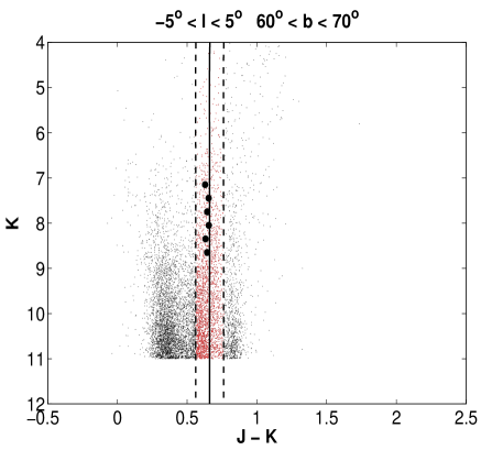
Figure 1: $K$ vs. $J-K$ 2MASS colour-magnitude diagram for the field centred at $l=0^{\circ}$. The fitted trace that we assign to RC giants population (solid line) and the limits for extraction of the stars (dashed lines) are also shown (see Sect. 2 in Cabrera-Lavers et al. (2005) for details).

The possible contamination due to dwarf stars in the extracted counts is the more restrictive issue when applying the method. To minimize this effect, we extracted only stars up to $m_{K}<$10 from the CMDs. In this range, contamination is less than 10 per cent of the total number stars, and it is even lower for brighter apparent magnitudes (Cabrera-Lavers et al., 2005). A magnitude $m_{K}=10$ corresponds to a distance from the Sun of approximately 2.5 kpc for a RC star, suitable for analyzing the disc more than 1 kpc above the Galactic plane but unable to reach the range of distances where the halo dominates the counts. Thus, the following analysis is made ignoring this Galactic component.

Other aspects that affect the method, as the metallicity dependence of the colour of the RC population, any possible contamination of lower luminosity giants in the counts, or the Malmquist bias (Malmquist, 1920) in the absolute magnitude of the RC stars have been taken into account, and their possible effects in the results were deeply discussed in Sect. 3 of Cabrera-Lavers et al. (2005). In any case, the uncertainties are always lower than the one coming from the contamination of dwarf stars.

We have first collected 10 $\times$ 10 degree fields in the 2MASS catalogue centered at fixed Galactic longitudes (in $\Delta l=10^{\circ}$ bins), with 60${}^{\circ}\leq b\leq 70^{\circ}$. We have to average several fields to obtain a sufficient number of RC stars to build up a conspicuous feature in the CMD which could be easily identifiable. The densities extracted are fitted by a double exponential following eq. (1), for both the thin and thick discs, with the additional constraint of producing the same local disc space density for the thin disc as it was obtained previously in Cabrera-Lavers et al. (2005).

Therefore, we assume for the discs a distribution as follows:

$$\rho_{i}(R,z)=n_{i}\leavevmode\nobreak\ exp(-|z|/h_{z,i})\leavevmode\nobreak\ exp(-(R-R_{0})/H_{i}),\\$$ (1)

where $z=z_{\odot}+r\sin(b)$, $r$ is the distance to the object from the Sun, $b$ is the Galactic latitude, $z_{\odot}$ is the vertical distance of the Sun from the Galactic plane we assume to be 15 pc (Hammersley et al., 1994), $R$ is the projected of the Galactocentric distance on the Galactic plane, $R_{0}$ is the solar distance from the Galactic center (Reid, 1993, 8 kpc), $h_{z,i}$ and $H_{i}$ are the scaleheight and scalelength, respectively, and $n_{i}$ is the normalized density at the solar radius. The suffix $i$ takes the values 1 and 2 as long as the thin and thick discs are considered.

As this study focuses on the dependence of the scaleheight and solar normalization on the Galactic longitude, for the scalelengths of the thin and thick discs we used the values of 2.1 kpc (López-Corredoira et al., 2002) and 3 kpc (Cabrera-Lavers et al., 2005) respectively, which were also obtained with 2MASS data. In any case, it has to be noted that the range of Galactocentric distances covered along each line of sight is so small that the effect of changing the value of the radial scalelengths is negligible (Cabrera-Lavers et al., 2005). The possible implications of a different scalelength of the thick disc will be discussed in Section 4.2.

Fig. 2 shows stellar densities profiles extracted at four different Galactic longitudes, as an example of the application of the method, while the Galactic model parameters are given in Table 1. Columns (2) and (3) give the scaleheight of the thin and thick discs, respectively, while the local space density of the thick disc $(n_{2}/n_{1})$ is given in Col. (4). Error bars in the scaleheights come from the uncertainty in the double exponential fit, by assuming Poisson noise in the extracted counts and taking into account the uncertainty in the distance above the plane as we have grouped 10 $\times$ 10 degree fields.

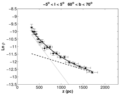
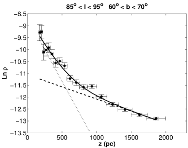
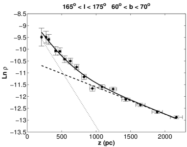
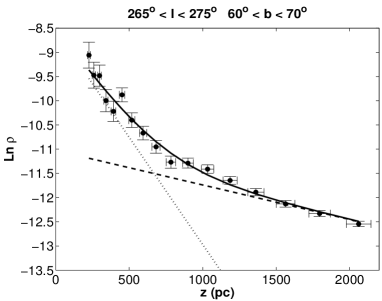
Figure 2: Density of red clump stars (in stars pc^-3) obtained from the CMDs for the Galactic longitudes of 0^∘, 90^∘, 170^∘, 270^∘. The best fits for a sum of thick disc (dashed line) and thin disc (dotted line) components are also shown as a solid line. Error bars come from the Poisson noise in the extracted counts and from the uncertainty in the distance above the plane.

Table 1: Galactic model parameters for the 36 star fields analyzed with 2MASS data.

	Thin disc	Thick disc
$<l>$ (∘)	$h_{z}$ (pc)	$h_{z}$ (pc)	$n_{2}/n_{1}\leavevmode\nobreak\ (\%)$
0	258$\pm$25	1127$\pm$142	10.79$\pm$2.71
10	209$\pm$18	1043$\pm$77	13.75$\pm$4.17
20	187$\pm$13	974$\pm$48	14.48$\pm$3.62
30	161$\pm$26	963$\pm$101	11.85$\pm$2.95
40	169$\pm$11	1074$\pm$70	9.63$\pm$2.41
50	197$\pm$ 7	909$\pm$38	8.08$\pm$2.02
60	202$\pm$22	943$\pm$90	9.21$\pm$2.31
70	185$\pm$13	904$\pm$92	9.69$\pm$2.43
80	248$\pm$19	914$\pm$60	11.83$\pm$4.71
90	191$\pm$12	994$\pm$82	6.19$\pm$1.54
100	180$\pm$22	754$\pm$65	12.97$\pm$3.18
110	269$\pm$25	922$\pm$139	11.03$\pm$2.76
120	211$\pm$20	933$\pm$68	11.61$\pm$3.40
130	140$\pm$18	807$\pm$57	7.79$\pm$1.94
140	165$\pm$13	949$\pm$65	8.34$\pm$2.08
150	221$\pm$16	827$\pm$67	13.97$\pm$3.51
160	167$\pm$17	848$\pm$71	11.26$\pm$3.90
170	214$\pm$14	872$\pm$58	12.52$\pm$3.89
180	183$\pm$14	839$\pm$54	12.24$\pm$3.07
190	143$\pm$18	815$\pm$33	9.99$\pm$3.48
200	172$\pm$19	807$\pm$51	12.81$\pm$3.94
210	186$\pm$13	956$\pm$66	10.31$\pm$2.59
220	160$\pm$17	959$\pm$103	9.32$\pm$2.34
230	199$\pm$16	1008$\pm$68	11.59$\pm$2.59
240	201$\pm$21	922$\pm$58	13.84$\pm$3.46
250	176$\pm$20	903$\pm$80	11.93$\pm$4.72
260	210$\pm$11	965$\pm$89	7.21$\pm$1.81
270	225$\pm$22	1003$\pm$36	8.83$\pm$1.52
280	197$\pm$20	1002$\pm$65	8.07$\pm$2.05
290	192$\pm$28	1005$\pm$120	9.75$\pm$3.46
300	198$\pm$23	991$\pm$129	13.59$\pm$3.40
310	209$\pm$15	1149$\pm$89	12.62$\pm$3.16
320	176$\pm$17	1155$\pm$106	11.09$\pm$2.85
330	214$\pm$16	1096$\pm$71	13.76$\pm$4.44
340	149$\pm$24	987$\pm$57	9.70$\pm$3.47
350	174$\pm$21	1066$\pm$80	10.94$\pm$2.74

3 Dependence of the Galactic model parameters with the Galactic longitude

Fig. 3 shows the variation of the scaleheight of the thin disc with the Galactic longitude. No obvious global trend is observed in the thin disc scaleheights, with a sample of values well compatible with a constant value of $<h_{z}>$=187 ($\sigma$=36) pc, well in agreement with usual estimates for this component (e.g., Bahcall & Soneira, 1984; Robin & Crézé, 1986; Reid & Majewski, 1993; Siegel et al., 2002; López-Corredoira et al., 2002). As shown in Fig. 3, we have overplotted a sinusoidal fit, no physical meaning, to the data. One can say that the scaleheight of the thin disc shows slight variation with the Galactic longitude. However, the scatter and the error bars are large, being compatible with a constant value independent of the Galactic longitude. Hence, we can conclude that the thin disc scaleheight is found to be a constant as a function of Galactic longitude.

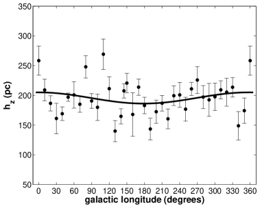
Figure 3: Variation of the scaleheight of the thin disc with the Galactic longitude.

For the thick disc the variation of the scaleheight with the Galactic longitude is more pronounced (Fig. 4). There is a maximum in the inner Galaxy ($|l|<30^{\circ}$), whereas in between $150^{\circ}<l<230^{\circ}$ there is a local minimum. The mean of the scaleheight for the data, $<h_{z}>=957$ ($\sigma$=100) pc is well within the given range found in the literature (Spagna et al., 1996; Ng et al., 1997; Buser, Rong & Karaali, 1998, 1999; Siegel et al., 2002; Larsen & Humphreys, 2003; Cabrera-Lavers et al., 2005).

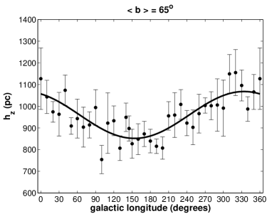
Figure 4: Variation of the scaleheight of the thick disc with the Galactic longitude.

The variation of the local space density of the thick disc relative to the local space density of the thin disc ($n_{2}/n_{1}$) with the Galactic longitude is given in Fig. 5. The trend gives a constant local space density, $(n_{2}/n_{1})\sim 10$ per cent, which confirms that the variation in $h_{z}$ in Fig. 4 is not an artifact of an anticorrelation in the local normalization (assuming, for example, a constant value $(n_{2}/n_{1})=10\%$ we still get the result in Fig. 4).

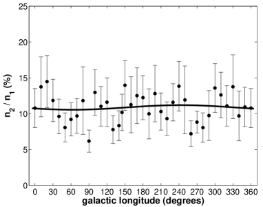
Figure 5: Variation of the relative space density of the thick disc with the Galactic longitude.

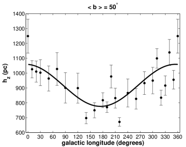
Figure 6: Variation of the scaleheight of the thick disc with the Galactic longitude, for fields with Galactic latitude $<b>=50^{\circ}$.

We checked the effect of the Galactic latitude on the variation of the scaleheight of the thick disc with the Galactic longitude for the 2MASS data. Fig. 6 shows the variation of the scaleheight with the Galactic longitude for fields at $<b>=50^{\circ}$. The trends in Figs. 4 and 6 are similar, although the zero points are different. The equations of the sinusoidal fits for the data in the fields with $<b>=50^{\circ}$ and $<b>=65^{\circ}$ are as follows:

$$h_{z}=918-141.45\leavevmode\nobreak\ \sin\leavevmode\nobreak\ (l-84.65^{\circ}),\leavevmode\nobreak\ \leavevmode\nobreak\ \leavevmode\nobreak\ \leavevmode\nobreak\ \leavevmode\nobreak\ \leavevmode\nobreak\ (at<b>=50^{\circ}),$$ (2)

$$h_{z}=959-108.02\leavevmode\nobreak\ \sin\leavevmode\nobreak\ (l-63.87^{\circ}),\leavevmode\nobreak\ \leavevmode\nobreak\ \leavevmode\nobreak\ \leavevmode\nobreak\ \leavevmode\nobreak\ \leavevmode\nobreak\ \leavevmode\nobreak\ (at<b>=65^{\circ}).$$ (3)

The difference between the scaleheights is larger (it amounts up to $\sim 100$ pc) for the longitudes corresponding to different minima in the two figures. No evident differences are found between the overall shape of the distributions. Hence the observed behaviour is associated to a global trend in the thick disc rather than to something exclusive of a restricted range of latitudes.

4 Discussion

4.1 Does the flare affect the scaleheight?

It is well known that the Galactic disc shows a flare, which produces an increase in the scaleheight as we move outwards in the Galaxy. In López-Corredoira et al. (2002) the flare was modelled by an exponential increase of $h_{z}$ with $R$, obtaining a law that approximately reproduced the observed counts up to $R<15$ kpc. On the contrary, for the inner Galaxy a flare with the opposite trend (an increase in $h_{z}$ as $R$ decreases) was found by López-Corredoira et al. (2004), who then proposed an expression that summarizes both regimes with a smooth transition between them:

$$h_{z}(R)=h_{z}(R_{\odot})\times[1+0.21(R-R_{\odot})+0.056(R-R_{\odot})^{2}]$$ (4)

The variation of the scaleheight of the thin and thick disc with Galactic longitude could be related with the flare itself. When the line of sight is pointing to the inner Galaxy ($|l|<30^{\circ}$) the mean Galactocentric distance of the sources is lower than when the line of sight is in the anticentre direction. We can then translate the $h_{z}$ vs. longitude plot in a $h_{z}$ vs. $R$ plot by deriving the mean Galactocentric distance to either the thin or thick disc sources, a procedure that is made by binning the data by the Galactocentric distance, R, and determining the mean radii of the red clump stars in each bin to average them. Figure 7 shows the variation in the scaleheight of the thin and thick disc with Galactocentric distance. It has to be noted that the range of Galactocentric distances is very small, so a possible derivation of parameters for the flare is far from being conclusive. We have compared López-Corredoira et al.’s law in both cases (dashed lines in the plot) considering $h_{z}$ ($R_{\odot})=200$ pc and $h_{z}$ $(R_{\odot})=900$ pc for the thin and thick disc, respectively. While the predictions for the thin disc are compatible with the data (although a constant value of $h_{z}$ can also fit the data), for the thick disc the observed trend is just the opposite with an increase of $h_{z}$ when moving to lower values of $R$ (represented by means of a linear fit on the lower panel of Fig. 7), a result that is in complete disagreement with the obtained for the outer thin disc (R$>$6 kpc) in López-Corredoira et al. (2002).

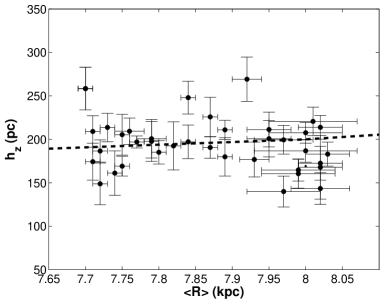
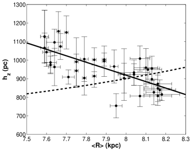
Figure 7: Variation in the scaleheight of the thin (above) and thick (below) discs with $R$.

To obtain a more accurate representation of the flare in the thick disc it would be necessary to increase the range of Galactocentric distances. For this reason, 2MASS data at $<b>=50^{\circ}$ are useful. They correspond to lines of sight at lower heights above the plane, thus the mean Galactocentric distance of the thick disc sources increases improving the fit. In Fig. 8 we show the variation in the scaleheight of the thick disc with respect to the mean Galactocentric distance, combining the results at $<b>=50^{\circ}$ (filled circles) with those at $<b>=65^{\circ}$ (open circles). By means of a linear fit to the data we obtain the following expression:

$$h_{z}(R)=(940\pm 20)\times[1-(0.12\pm 0.02)(R-R_{\odot})]\leavevmode\nobreak\ \leavevmode\nobreak\ \leavevmode\nobreak\ \leavevmode\nobreak\ \leavevmode\nobreak\ \leavevmode\nobreak\ (pc)$$ (5)

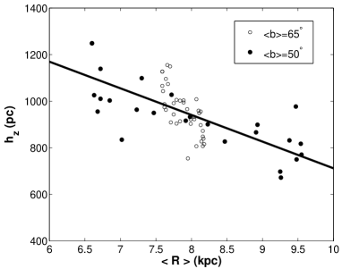
Figure 8: Variation of the scaleheight of the thick disc with $R$ by using 2MASS data at $<b>=50^{\circ}$ and $<b>=65^{\circ}$. The best linear fit to the observed trend is also shown.

It is not so common to observe an increase of the scaleheight as we move to the inner Galaxy. Furthermore, no similar analysis of a possible flare in the thick disc is found in the literature. In a very recent article, Momany et al. (2006) analysed the warp and flare of the disc of the Milky Way but only concentrated in those related to the thin disc. By using red giant branch stars in the range $0.45<z<2.25$ kpc they obtained a slight increase of the scaleheight of the disc with increasing Galactocentric radii, up to $R\sim$15 kpc (their fig. 15). They claimed that the overall mean scaleheight around 0.65 kpc they obtained was a reflection of a mixture of the thin and thick disc populations. If we put together the known trend in the scaleheight of the thin disc (that is, an increasing $h_{z}$ as $R$ increases) with the result obtained in this paper for the thick disc (an increase in $h_{z}$ as $R$ decreases), one must expect that a sort of ’cancellation’ appears, producing a nearly constant $h_{z}$ at intermediate heights above the plane.

To check this possibility, we have made a simple simulation for a combination of a thin disc with the density laws of López-Corredoira et al. (2004) and a thick disc with an increase in $h_{z}$ represented by eq. (5) and a relative space density of 10 per cent of the thin disc according to Cabrera-Lavers et al. (2005). The resulting densities are fitted by a single exponential law (as if only one component were present), obtaining in that way the expected variation in scaleheight with the Galactocentric distance.

When comparing this simulation with the data taken from Momany et al. (2006) (Fig. 9) a good agreement is observed. In the range of distances $4<R<9$ kpc a nearly constant scaleheight is expected that is not far from that observed (note we did not perform any kind of fit to Momany et al.’s data, so the coincidence in the value for $h_{z}$ at $4<R<7$ kpc is very interesting). Predicted values for $R>10$ kpc are larger than those, but it was expected due to the excessively high increase in $h_{z}$ for the thin disc that López-Corredoira et al.’s model produces in this range of Galactocentric distances. A more modest increase in $h_{z}$ with $R$ for the thin disc (as obtained in Alves (2000) or in Momany et al. (2006)) would produce a better agreement with the data, but this was beyond the scope of this comparison. For $R<4$ kpc, again an excessive increase in $h_{z}$ is obtained in the simulation, but again it was known that the validity of López-Corredoira et al.’s model for $R<2.5$ kpc is not well demonstrated.

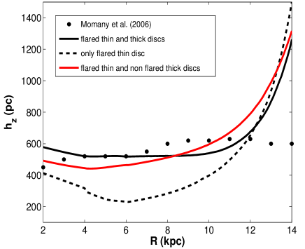
Figure 9: Variation of the scaleheight with $R$ taken from the work of Momany et al. (2006) compared with the simulations of different possible combinations of thin and thick disc densities, following the results of López-Corredoira et al. (2004) (for the thin disc) and this paper (for the thick disc).

We have also introduced some changes in the simulation. By eliminating the contribution of the thick disc (that is, assuming that only the thin disc is observed) we recovered the predictions of the López-Corredoira et al.’s model, with the scaleheight corresponding to the thin disc (dashed line in Fig. 9). It is even more remarkable how when a flaring in the thick disc is neglected (assuming a constant scaleheight of 940 pc for this component) the trend obtained still follows the increase in the scaleheight due the thin disc, but with higher $h_{z}$ values as corresponds with the mixing of both populations (grey solid line in Fig. 9). The result is also less sensitive to other parameters, as the relative space density of the thick disc (no changes were obtained by varying it from 5 to 15 per cent) or the value of $R_{\odot}$ (assumed as 8 kpc).

A combination of a flared thin disc and a flared thick disc with opposite trends seems, then, to be compatible with the observed scaleheights at intermediate heights above the plane, as those of Momany et al. (2006). Thus, the observed variation in the scaleheight of the thick disc with the galactic longitude has been obtained here as expected.

4.2 Effect of the scalelength of the thick disc

In Section 2.1 we addressed what we considered a fixed scalelength of 3 kpc for the thick disc, as obtained in Cabrera-Lavers et al. (2005). However, a different scalelength would reproduce the observed variation in the scaleheight without the need for a flare in the disc itself. For example, a shorter scalelength of 2 kpc for the thick disc would increase the predicted star counts in the inner disc and reduce them in the outer disc, relative to the assumed 3 kpc scalelength, simulating a higher scaleheight in the inner disc and a lower scaleheight in the outer disc, as was found in Section 4.

However, the effect of the scalelength on the derived densities is negligible, as we are moving in a very narrow range of Galactocentric distances. To reproduce the same density as that resulting from a scalelength of 3 kpc and a scaleheight of 1100 pc, like those derived in the inner Galaxy but with a constant scaleheight of 800 pc, the scalelength has to change by a factor $\sim$1.4 with respect to the assumed value of 3 kpc (that is, around 4.2 kpc), a value that is 11$\sigma$ above that derived in Cabrera-Lavers et al. (2005).

In order to check this statement, we repeated the analysis of Section 2 in a series of nine test fields but now assuming two different scalelengths for the thick disc: $H$ = 2 kpc and $H$ = 2.5 kpc, respectively. The results are shown in Fig. 10, together with sinusoidal fits to the data. The observed trend is nearly coincident with that of Fig. 4 in both amplitude and the positions of the minima. Hence, the effect of a different scalelength from the assumed one of 3 kpc has to be discarded as being responsible for the results discussed in this paper.

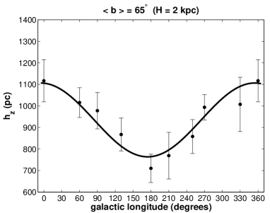
Figure 10: Variation in the scaleheight of the thick disc with the Galactic longitude obtained by assuming a scalelength of $H$=2 kpc (above) or $H$=2.5 kpc for this component (below).

5 Conclusion

By using NIR data from 2MASS we have observed significant changes in the structural parameters of the thin and thick discs of the Milky Way, that are more than simple fluctuations caused by model fitting to the data.

A plausible explanation for the observed changes in the scaleheight of the discs arises from the combined effect of the warp and flare in the Galactic thin and thick disc, which displaces both structures from the assumed position expected for a “smooth disc” (that is, a flat, azimuthally homogeneus and constant scaleheight disc). This implies that in some directions the effect is more noticeable than in others, producing variations in the parameters resulting from a fit of a single Galactic model. The observed trend in the change of the scaleheight with galactic longitude is well reproducible theoretically by assuming the accretion of intergalactic matter on to the Galactic disc, which in general produces a different pressure depending on both the Galactocentric radius and azimuth, the same pressure which would also be responsible for the formation of S-warps and/or U-warps in galaxies (López-Corredoira, Betancort-Rijo & Beckman, 2002). The pressure would be similar to a piston mechanism, only from one side of the disc (Sánchez-Salcedo, 2006, §4.6). As a result of this mechanism the scaleheight of the disc would present a similar shape to that obtained in Figure 4. However, it is far from our intention to consider that our result is a demonstration that this speculative hypothesis is the correct one in explaining the uncertain origin for the Milky Way’s flare and warp; but it is consistent with the observed data.

The flare obtained in the thick disc from 2MASS data has an opposite trend to that commonly assumed for the thin disc, with a scaleheight that increases as we move to the innermost Galaxy, being the first time that a possible flare in this Galactic component is observed. It is beyond the scope of this paper to determine from the observed results a theoretical scenario that supports the origin of this possible flare, although some asymmetries in the thick disc hve been well known for some time now (Parker et al., 2003). We suspect that the different behaviour in the inner Galaxy is related to the interaction of the 4 kpc inner Galactic bar (López-Corredoira et al., 2006) with its surroundings. However, it is more difficult to explain the possible effect of this component on the thick disc, although some known asymmetries of this component have been suggested as having been caused by the Galactic bar (Parker et al., 2004). Unfortunately, we do not have enough information to add anything in this regard. Probably, kinematic analyses by using radial velocity data as those provided by the Sloan Extension for Galactic Understanding and Exploration (SEGUE, Newberg et al., 2003) or the Radial Velocity Experiment (RAVE, Steinmetz et al., 2006) will be very valuable to go deeper in this topic.