A highly obscured and strongly clustered galaxy population discovered with the Spitzer Space Telescope

Abstract

The $\sim 800$ optically unseen ($R>25.5$) 24$\,\mu$m-selected sources in the complete Spitzer First Look Survey sample (Fadda et al. 2006) with $F_{24\mu\rm m}\geq 0.35\,$mJy are found to be very strongly clustered. If, as indicated by several lines of circumstantial evidence, they are ultraluminous far-IR galaxies at $z\simeq 1.6$–2.7, the amplitude of their spatial correlation function is very high. The associated comoving clustering length is estimated to be $r_{0}=14.0_{-2.4}^{+2.1}$ Mpc, value which puts these sources amongst the most strongly clustered populations of our known universe. Their $8\,\mu$m–$24\,\mu$m colours suggest that the AGN contribution dominates above $F_{24\mu\rm m}\simeq 0.8\,$mJy, consistent with earlier analyses. The properties of these objects (number counts, redshift distribution, clustering amplitude) are fully consistent with those of proto-spheroidal galaxies in the process of forming most of their stars and of growing their active nucleus, as described by the Granato et al. (2004) model. In particular, the inferred space density of such galaxies at $z\simeq 2$ is much higher than what expected from most semi-analytic models.
Matches of the observed projected correlation function $w(\theta)$ with models derived within the so-called Halo Occupation Scenario show that these sources have to be hosted by haloes more massive than $\simeq 10^{13.4}M_{\odot}$. This value is significantly higher than that for the typical galactic haloes hosting massive elliptical galaxies, suggesting a duration of the starburst phase of massive high-redshift dusty galaxies of $T_{B}\sim 0.5$ Gyr.

1 Introduction

Understanding the assembly history of massive spheroidal galaxies is a key issue for galaxy formation models. The “naive” expectation from the canonical hierarchical merging scenario, that proved to be remarkably successful in explaining many aspects of large-scale structure formation, is that massive galaxies generally form late and over a long period of time as the result of many mergers of smaller haloes. On the other hand, there is quite extensive evidence that massive galaxies may form at high redshifts and on short timescales (see, e.g. Cimatti et al. 2004; Fontana et al. 2004; Glazebrook et al. 2004; Giallongo et al. 2005; Treu et al. 2005; Saracco et al. 2006; Bundy et al. 2006), while the sites of active star formation shift to lower mass systems at later epochs, a pattern referred to as ”downsizing” (Cowie et al. 1996). In order to reconcile the observational evidence that stellar populations in large spheroidal galaxies are old and essentially coeval (Ellis et al. 1997; Holden et al. 2005) with the hierarchical merging scenario, the possibility of mergers of evolved sub-units (“dry mergers”) has been introduced (van Dokkum et al. 2005; Faber et al. 2006; Naab et al. 2006). This mechanism is however strongly disfavoured by studies on the evolution of the stellar mass function (Bundy et al. 2006).

Key information, complementary to optical/IR data, has come from sub-millimeter surveys (Hughes et al. 1998; Eales et al. 2000; Knudsen et al. 2006) which have found a large population of luminous sources at substantial redshifts (Chapman et al. 2005). However, the interpretation of this class of objects is still controversial (e.g. Granato et al. 2004; Kaviani et al. 2003; Baugh et al. 2005).

The heart of the problem are the masses of the objects: a large fraction of present day massive galaxies already assembled at $z\sim 2-3$ would be extremely challenging for the standard view of a merging-driven growth. Measurements of clustering amplitudes are a unique tool to estimate halo masses at high $z$, but complete samples comprising at least several hundreds of sources are necessary. This is far more than what detected by sub-mm surveys, that have therefore only provided tentative clustering estimates (Blain et al. 2005).

Here we report evidence of strong clustering for the optically very faint ($R>25.5$) sources included in the complete $24\,\mu$m sample obtained from the Spitzer first cosmological survey (Fadda et al. 2006). Comparisons with template spectral energy distributions and up-to-date models for galaxy formation and evolution set these objects at $z\sim 2$. The clustering properties and the counts of such sources are consistent with them being very massive proto-spheroidal galaxies in the process of forming most of their stars. Their comoving number density appears to be much higher than what expected from most semi-analytic models.

The layout of the paper is as follows. In § 2 we describe the sample selection. In § 3 we investigate the source photometric and spectroscopic properties. In § 4 we derive the two point angular correlation function, while in § 5 we present its implications for source properties, and in particular for their halo masses, in the light of the so-called Halo Occupation Model. Comparisons with model predictions are dealt with in § 6. Our main conclusions are summarized in § 7.

Throughout this work we adopt a flat cosmology with a matter density $\Omega_{m}=0.3$ and a vacuum energy density $\Omega_{\Lambda}=0.7$, a present-day value of the Hubble parameter in units of $100$ km/s/Mpc $h=0.7$, and rms density fluctuations within a sphere of $8h^{-1}$ Mpc radius $\sigma_{8}=0.8$ (Spergel et al. 2003).

2 The sample selection

2.1 The Parent Catalogue

Our analysis is based on the 24$\,\mu$m data obtained during the first cosmological survey performed by the Spitzer Space Telescope (First Look Survey). Observations and data reduction are extensively described in Fadda et al. (2006). Briefly, the survey consists of a shallow observation of a $2.5^{\circ}\times 2^{\circ}$ area centered at $(17^{h}18^{m},+59^{\circ}30^{\prime})$ (main survey) and of a deeper observation on a smaller region of the sky (verification survey) overlapping with the first one.

Observations were performed using the MIPS (Multi Imaging Photometer for Spitzer, Rieke et al. 2004), whose spatial resolution at 24$\,\mu$m is 5.9^′′ FWHM. Approximately $\sim 17000$ sources have been extracted with signal-to-noise-ratio (SNR) greater than five down to $\sim 0.2$ mJy in the main survey and to $\sim 0.1$ mJy in the verification survey. Astrometric errors depend on the SNR, varying between $0.35^{\prime\prime}$ and $1.1^{\prime\prime}$ for sources detected at 20–5$\sigma$levels. The main survey is estimated to be $>90$% complete down to a limiting flux $F_{24\mu\rm m}=0.35$ mJy (Fadda et al. 2006).

Optical counterparts have been obtained by Fadda et al. (2006) for most of the 24$\,\mu$m sources by cross-correlating galaxies in the MIPS catalogue with the $R$-band KPNO observations of Fadda et al. (2004) and – for objects with $R\leq 18$ – with sources from the Sloan Digital Sky Survey (Hogg et al., in preparation). These two optical data-sets cover in a roughly homogeneous way most of the area probed by the 24$\,\mu$m main survey, except for three corners. The typical limiting magnitude of the joint SDSS+KPNO observations is $R=25.5$, and $\sim 82\%$ of the 24$\,\mu$m of all sources in the MIPS survey are reported to have an optical counterpart brighter than this limit.

Despite ongoing efforts (Marleau et al. 2003; Choi et al. 2006; Yan et al. 2005), there is still no homogeneous redshift information on the sources making up the MIPS 24$\,\mu$m catalogue, except for a very small area overlapping with the GOODS/CDFS field (Caputi et al. 2006). However, redshift estimates can be obtained from photometric data, taking advantage of the Spitzer Infrared Array Camera (IRAC) survey which covers an extensive portion of the MIPS field (Lacy et al. 2005).

The main IRAC survey has covered an area of 3.8 square degrees in the four channels centered at 3.6, 4.5, 5.8 and 8$\,\mu$m, reaching a $\sim 100$% completeness level respectively at $\sim 40$, $\sim 40$, $\sim 100$ and $\sim 100~{}\mu$Jy (Fig. 3 of Lacy et al. 2005). The positional accuracy goes from $\sim 0.25^{\prime\prime}$ for high signal-to-noise sources to 1^′′ at the lowest flux levels.

Investigations of the Spectral Energy Distributions (SED) of prototype sources such as M 82, Arp 220, and Mkn 231 (the latter with mid-IR luminosity probably powered by the presence of an AGN) shows that the tightest constraints on the redshifts of very distant galaxies with intense star-formation come from the 8$\,\mu$m IRAC channel, since such sources are expected to be very weak at shorter wavelengths (see also Yan et al. 2005). Therefore, in the following we will only consider data from the 8$\,\mu$m channel.

2.2 Matching procedure

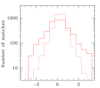
Figure 1: Distribution of the residuals $\Delta x=$RA${}_{24\mu\rm m}-$RA_8μm (solid line) and $\Delta y$=Dec${}_{24\mu\rm m}-$Dec_8μm (dashed line) between 24$\,\mu$m and 8$\,\mu$m positions.

We have looked for the 8$\,\mu$m counterparts to MIPS sources over the 2.85 square degrees region $257.7^{\circ}\mathrel{\hbox to0.0pt{\lower 3.0pt\hbox{$\sim$}\hss}\raise 2.0pt\hbox{$<$}}$ RA(2000) $\mathrel{\hbox to0.0pt{\lower 3.0pt\hbox{$\sim$}\hss}\raise 2.0pt\hbox{$<$}}261^{\circ}$ and 58.6${}^{\circ}\mathrel{\hbox to0.0pt{\lower 3.0pt\hbox{$\sim$}\hss}\raise 2.0pt\hbox{$<$}}$ Dec $\mathrel{\hbox to0.0pt{\lower 3.0pt\hbox{$\sim$}\hss}\raise 2.0pt\hbox{$<$}}60.3^{\circ}$, for which both 8$\,\mu$m and $R$-band observations are available. In this area there are 7592 24$\,\mu$m sources and 8,646 8$\,\mu$m sources above the respective completeness limits of 0.35 mJy and 0.1 mJy.

We identified as the counterpart to a MIPS source the IRAC source with a positional separation less than a suitably chosen radius. As mentioned in § 2.1, the positional accuracies for both MIPS and IRAC sources with $\hbox{SNR}=5$ is $\simeq 1^{\prime\prime}$, so that we expect a rms positional difference due to astrometric errors of $\sim\sqrt{2^{\prime\prime}}\simeq 1.4^{\prime\prime}$. Moreover, the IRAC astrometry is based on 2MASS, while that of the 24$\,\mu$m sources is related to SDSS. Although both systems are very accurate, a small systematic offset may be present.

Tackling the problem from a more pragmatic point of view, we considered the distribution of the residuals $\Delta x={\rm RA}_{24\mu\rm m}-{\rm RA}_{8\mu\rm m}$, $\Delta y={\rm Dec}_{24\mu\rm m}-{\rm Dec}_{8\mu\rm m}$ between the positions of all 24$\,\mu$m and 8$\,\mu$m pairs with separations $|\Delta x|$ and $|\Delta y|$ less than $5^{\prime\prime}$. The distribution of residuals shows a strong concentration of points near $\Delta x\simeq-0.14$ and $\Delta y\simeq 2.24\cdot 10^{-3}$ arcsec, values which can be taken as the mean positional offsets between the 24$\,\mu$m and 8$\,\mu$m reference frames.

We have corrected for this effect and in Fig. 1 we plot the histogram of the number of matches as a function of $\Delta x$ (solid line) and $\Delta y$ (dashed line) offsets. The distributions now correctly peaks near zero offset with a rms value of about $1^{\prime\prime}.5$, in agreement with the above simple estimate. We have then chosen a $3^{\prime\prime}$ matching radius – equivalent to about $2\sigma$ – which should therefore include $\sim 95\%$ of the true identifications. The probability that an 8$\,\mu$m source falls by chance within the search radius from a 24$\,\mu$m source (equal to the surface density of 8$\mu$m sources times the area within such radius) is $\simeq 6.6\times 10^{-3}$. Increasing the matching radius increases the number of interlopers more than that of true counterparts.

The above procedure yielded 3429 $F_{24\mu\rm m}\geq 0.35$ mJy 24$\,\mu$m sources endowed with an 8$\,\mu$m counterpart. Given the completeness limit of the IRAC survey, we will then assume the remaining MIPS objects to have an 8$\,\mu$m counterpart fainter than 0.1 mJy.

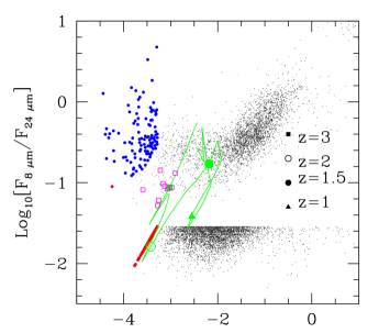
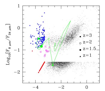
Figure 2: Distribution of the 8$\,\mu$m to 24$\,\mu$m vs the 0.7$\,\mu$m to 24$\,\mu$m flux ratios for the 7592 $F_{24\mu\rm m}\geq 0.35$ mJy MIPS sources in the $2.85\,\hbox{deg}^{2}$ region covered by both the KPNO and the IRAC surveys. These are compared with the computed colour-colour tracks as a function of redshift (green solid lines) for the Arp 220 (left-hand panel) and the Mkn 231 (right-hand panel) SEDs. For sake of clarity, objects with an 8$\,\mu$m counterpart fainter than 0.1 mJy have been given $F_{8\mu\rm m}=10^{-2}$ mJy and are responsible for the apparent gap observed in the distribution along the $y$ axis, while sources without an optical counterpart in the KPNO catalogue have been attributed $R=25.5$ and are represented by the filled circles. Blue circles indicate objects with $F_{8\mu\rm m}/F_{24\mu\rm m}>0.1$, while the red ones are for those with $F_{8\mu\rm m}/F_{24\mu\rm m}<0.1$. Note that, although this in not clear from the figure, because many red points are piling up in the same spot, objects with $F_{8\mu\rm m}/F_{24\mu\rm m}<0.1$ are much more numerous than those with $F_{8\mu\rm m}/F_{24\mu\rm m}>0.1$. Open squares represent sources from the Pope et al. (2006) sample with $F_{24\mu\rm m}\geq 0.15$ mJy.

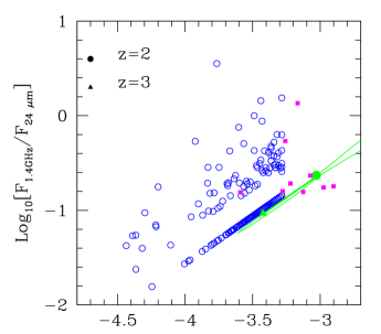
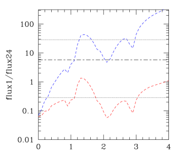
Figure 3: Left-hand panel: distribution of the 1.4 GHz to $24\,\mu{\rm m}$ vs the $0.7\,\mu{\rm m}$ to $24\,\mu{\rm m}$ flux ratios for the 793 $F_{24\mu\rm m}\geq 0.35$ mJy, $R>25.5$ MIPS sources present in the $3.97\,\hbox{deg}^{2}$ region considered in this work. For sake of clarity, objects fainter than the 0.1 mJy detection limit at 1.4 GHz have been attributed $F_{1.4\rm GHz}=5\cdot 10^{-2}\,$ mJy and produce the diagonal line on the bottom right corner of the plot. Sources undetected by the KPNO survey have been assigned $R=25.5$. The filled squares indicate objects from the Pope et al. (2006) sample with $F_{24\mu\rm m}\geq 0.15\,$mJy, while the solid (green) line shows the track, as a function of redshift, yielded by the Arp 220 SED. Right-hand panel: redshift dependence of the $F_{850\mu\rm m}/F_{24\mu\rm m}$ (upper curve) and $F_{1.4\rm GHz}/F_{24\mu\rm m}$ (lower curve) flux density ratios for the Arp 220 SED. The upper dotted line shows the ratio between the limiting fluxes of our sample ($F_{24\mu\rm m}=0.35$ mJy) and of the dataset by Sawicki & Webb (2005; $F_{850\mu\rm m}=10$ mJy), while the short-long dashed one corresponds to decreasing $F_{850\mu\rm m}$ to 2 mJy. The lower dotted line is the ratio between the limiting 24$\mu$m and 1.4 GHz fluxes ($F_{1.4\rm GHz}=0.1$) for our sample.

3 Photometric and spectroscopic properties

The distribution of 8$\,\mu$m to 24$\,\mu$m vs 0.7$\,\mu$m to 24$\,\mu$m flux ratios for all the 7592 $F_{24\mu\rm m}\geq 0.35$ mJy MIPS sources in the $2.85\,\hbox{deg}^{2}$ region covered by both the KPNO and the IRAC surveys is reported in Fig. 2. $R$ magnitudes have been converted to 0.7$\mu$m fluxes using the calibration in Fukugita, Shimasaku & Ichikawa (1995). For sake of clarity, objects with an 8$\,\mu$m counterpart fainter than 0.1 mJy have been given $F_{8\mu\rm m}=10^{-2}$ mJy and are responsible for the apparent gap observed in the lower part of the $F_{8\mu\rm m}/F_{24\mu\rm m}$ axis, while sources without an optical counterpart in the KPNO catalogue have all been given R=25.5 and are represented by the red or blue filled circles. Blue circles indicate objects with $F_{8\mu\rm m}/F_{24\mu\rm m}>0.1$, while the red ones are for those with $F_{8\mu\rm m}/F_{24\mu\rm m}<0.1$.

The solid (green) lines show, as a function of redshift, the colours corresponding to the SEDs of Arp 220 (left-hand panel), a well studied local starburst galaxy – featuring in its mid-IR spectrum signatures of heavy dust absorption (Spoon et al. 2004) – found to provide to a first approximation a good template to describe the energy output of high-redshift galaxies undergoing intense star-formation (see e.g. Pope et al. 2006), and of Mkn 231 (right-hand panel), a prototype absorbed AGN dominating the mid-IR emission, hosted in a galaxy with very intense star formation. This figure shows that, for both source types, extreme 24$\mu$m to $R$-band flux ratios (or $R>25.5$) likely correspond to sources at $z\simeq 1.6$–3.

This conclusion is supported by the comparison of the distribution of the $F_{1.4\rm GHz}/F_{24\mu\rm m}$ vs $F_{0.7\mu\rm m}/F_{24\mu\rm m}$ colours for the $R>25.5$ sources from the complete MIPS sample with the track, as a function of redshift, yielded by the Arp 220 SED (left-hand panel of Fig. 3). Radio data come from the $20$ cm radio survey performed by Condon et al. (2003) on 82% of the 24$\,\mu$m field down to a limiting flux of 0.1 mJy. Only 86 out of the 793 $R>25.5$, $F_{24\mu\rm m}\geq 0.35$ mJy sources (11% of the sample) are detected. The lower dashed curve in the right-hand panel of Fig. 3 details the redshift dependence of the $F_{1.4\rm GHz}/F_{24\mu\rm m}$ ratio for the Arp 220 SED, showing that sources undergoing intense star-formation and endowed with 24$\,\mu$m fluxes close to the MIPS detection limit, present 1.4 GHz fluxes below the 0.1 mJy threshold of Condon’s survey only if $z<1.2$ or $1.7\leq z\leq 3$. Combining this latter piece of information with the trend of the $F_{1.4\rm GHz}/F_{24\mu\rm m}$ vs $F_{0.7\mu\rm m}/F_{24\mu\rm m}$ distribution, we can conclude that most of the $R>25.5$ MIPS sources are consistent with them being starburst galaxies placed in the redshift range $1.6\mathrel{\hbox to0.0pt{\lower 3.0pt\hbox{$\sim$}\hss}\raise 2.0pt\hbox{$<$}}z\mathrel{\hbox to0.0pt{\lower 3.0pt\hbox{$\sim$}\hss}\raise 2.0pt\hbox{$<$}}3$. Although the above arguments do not exclude the possibility that some of our sources are actually at $z\simeq 1$, a really extreme extinction would be required to make them fainter than $R=25.5$, and therefore such sources must be very rare. This is directly confirmed by the spectroscopic observations summarized below, that did not find $R\geq 25.5$ objects at $z<1.7$.

The upper dashed curve in the right-hand panel of Fig. 3 shows that galaxies with a SED similar to Arp 220, fluxes $F_{24\mu\rm m}\simeq 0.35\,$mJy, and lying in the redshift range $1.6\leq z\leq 3$ have $F_{850\mu\rm m}\mathrel{\hbox to0.0pt{\lower 3.0pt\hbox{$\sim$}\hss}\raise 2.0pt\hbox{$<$}}12$ mJy. As pointed out by Houck et al. (2005), sources with higher AGN contribution (in general brighter at 24$\,\mu\rm m$ than the above limit) which therefore present hotter dust, exhibit $F_{850\mu\rm m}/F_{24\mu\rm m}$ ratios lower by a typical factor of 3–5 than those of (sub)-mm selected sources ($F_{850\mu\rm m}/F_{24\mu\rm m}\simeq 5$; see e.g. Lutz et al. 2005), generally high-$z$ starburst galaxies (Ivison et al. 2004; Egami et al. 2004; Frayer et al. 2004; Charmandaris et al. 2004; Pope et al. 2006). A small fraction (151 arcmin²) of the area covered by the First Look Survey has been observed by Sawicki & Webb (2005) with SCUBA on JCMT. These authors report the detection ($S/N>3.5$) of ten sources with $F_{850\mu{\rm m}}\geq 10$ mJy. As expected on the basis of the above discussion, none of them belongs to the complete sample of $R>25.5$ MIPS sources although one of the detected objects is just below the 0.35 mJy limit (J171736.9+593354, $F_{24\mu\rm m}=0.32$ mJy).

Thus, radio, sub-mm, mid-IR and optical photometric data converge in indicating that the process of extracting optically faint sources from samples selected at 24$\,\mu\rm m$ singles out star-forming galaxies in the redshift range $1.6\mathrel{\hbox to0.0pt{\lower 3.0pt\hbox{$\sim$}\hss}\raise 2.0pt\hbox{$<$}}z\mathrel{\hbox to0.0pt{\lower 3.0pt\hbox{$\sim$}\hss}\raise 2.0pt\hbox{$<$}}3$. As pointed out by Houck et al. (2005) such a redshift range is determined by well established selection effects. The requirement for the sources to be optically very faint ($R>25.5$) forces them to $z\geq 1$, because obscuration is higher in the rest-frame UV. On the other hand, the deep and broad $9.7\,\mu$m silicate absorption feature, which is common in ultra-luminous infrared galaxies (Armus et al. 2004; Higdon et al. 2004; Spoon et al. 2004) works against inclusion in $24\,\mu$m-selected samples of objects in the redshift range $1\mathrel{\hbox to0.0pt{\lower 3.0pt\hbox{$\sim$}\hss}\raise 2.0pt\hbox{$<$}}z\mathrel{\hbox to0.0pt{\lower 3.0pt\hbox{$\sim$}\hss}\raise 2.0pt\hbox{$<$}}1.6$, while the strongest PAH emission feature (set in the rest-frame at $\lambda=7.7\mu$m) enters the $24\,\mu$m filter at $z\sim 2.1$, and another relatively strong PAH line ($\lambda=6.2\mu$m) appears at 24$\,\mu\rm m$ for $z\sim 2.9$. Ultra-luminous IR galaxies at still higher redshifts are expected to become increasingly rare because of the dearth of very massive galactic haloes.

The above conclusion is fully borne out by spectroscopic data, although only obtained for a limited number of sources. Yan et al. (2005) obtained low-resolution spectra with the Spitzer InfraRed Spectrograph (IRS) for eight First Look Survey sources with 24$\mu$m fluxes brighter than 0.9 mJy. Further colour constraints which were applied include: $\log_{10}(\nu F_{\nu}(24\rm\mu m)/\nu F_{\nu}(8\rm\mu m))\geq 0.5$ and $\log_{10}(\nu F_{\nu}(24\rm\mu m)/\nu F_{\nu}(0.7\rm\mu m))\geq 1.0$. Three of these sources (namely IRS2, IRS8, and IRS9) have $R>25.5$. All three lie in the redshift range $1.8\mathrel{\hbox to0.0pt{\lower 3.0pt\hbox{$\sim$}\hss}\raise 2.0pt\hbox{$<$}}z\mathrel{\hbox to0.0pt{\lower 3.0pt\hbox{$\sim$}\hss}\raise 2.0pt\hbox{$<$}}2.6$ ($z_{\rm IRS2}=2.34$; $z_{\rm IRS8}=2.6$; $z_{\rm IRS9}=1.8$). IRS2 and IRS9 show strong PAH emission lines and moderate silicate absorption in their spectra, while IRS8 only presents strong silicate absorption. IRS9 has also been observed with MIPS at 70$\mu$m and with MAMBO at 1.2 mm, and found to have fluxes of respectively 42 mJy and 2.5 mJy. The estimated bolometric luminosities (Yan et al. 2005) are $L_{\rm bol}=1.83\cdot 10^{13}L_{\odot}$ (IRS9), $L_{\rm bol}=4.3\cdot 10^{13}L_{\odot}$ (IRS2), and $L_{\rm bol}=2\cdot 10^{13}L_{\odot}$ (IRS8).

Houck et al. (2005) used the Spitzer Telescope to image at 24$\,\mu$m a $9\,\hbox{deg}^{2}$ field within the NOAO Deep Wide-Field Survey region down to a flux of 0.3 mJy. Thirty-one sources, with $F_{24\mu\rm m}\geq 0.75$ mJy and $R\geq 24.5$ have further been observed with the IRS. Redshift determinations were possible for 17 of them, including 13 sources with $R>25.5$. Again, the measured redshifts are all in the range $1.7<z<2.6$, except possibly for one object which appears to have $z=0.7$, but this is the least secure determination due to a poor spectrum beyond 30$\mu$m.

Eighteen optically faint ($R>23.9$) sources from the Spitzer First Look Survey, with $F_{24\mu\rm m}>1$ mJy and 20 cm detections to a limit of $115\,\mu$Jy, have been observed with the IRS by Weedman et al. (2006). All sources with $R>24$ lie in the range $1.7<z<2.5$.

Furthermore, Pope et al. (2006) have recently presented 24$\,\mu$m observations of 35 sub-mm selected sources with 850$\mu$m fluxes $\mathrel{\hbox to0.0pt{\lower 3.0pt\hbox{$\sim$}\hss}\raise 2.0pt\hbox{$>$}}2$ mJy. Nine of these sources have 24$\,\mu$m fluxes brighter than 0.15 mJy, the limit of the First Look Survey in the verification region, and $i_{\rm AB}\geq 24$ (7 have $i_{\rm AB}\geq 26.2$). All of them have spectroscopic or photometric redshifts in the range $z\sim[1.7-2.7]$. Their colours, shown in Fig. 2 by the magenta open squares and in the left-hand panel of Fig. 3 by filled squares, lie in those regions identified by the $F_{24\mu\rm m}\geq 0.35$ mJy and $R>25.5$ MIPS objects, confirming that the above selection singles out galaxies with properties similar to those detected by (sub)-mm surveys.

On the basis of the above results obtained on both photometric and spectroscopic grounds, we can then confidently assume that sources with $F_{24\mu\rm m}\geq 0.35$ mJy and $R>25.5$ typically identify star-forming galaxies in the redshift interval $1.6\mathrel{\hbox to0.0pt{\lower 3.0pt\hbox{$\sim$}\hss}\raise 2.0pt\hbox{$<$}}z\mathrel{\hbox to0.0pt{\lower 3.0pt\hbox{$\sim$}\hss}\raise 2.0pt\hbox{$<$}}3$. Such a conclusion will be further strengthened in § 6, in the light of the most up-to-date models for galaxy formation and evolution.

3.1 Starburst vs AGN components

There are 510 sources with $R>25.5$ and $F_{24\mu\rm m}\geq 0.35$ mJy in the $2.85\,\hbox{deg}^{2}$ region where both 24 $\mu$m and 8 $\mu$m data are available (see § 2.2). Figure 2 illustrates that, for $z\simeq 1.5$–3, “AGN-dominated” and “starburst-dominated” SEDs have different $F_{8\mu\rm m}/F_{24\mu\rm m}$ ratios, the dividing line being set at $F_{8\mu\rm m}/F_{24\mu\rm m}\simeq 0.1$ (see also Yan et al. 2005): starburst galaxies (Arp 220-like SED) are generally below this value, while AGN-powered sources (Mkn 231-like SED) are above it. Most (401) of the 510 sources within the overlapping IRAC-MIPS area present $F_{8\mu\rm m}/F_{24\mu\rm m}<0.1$ so that – to a first order – can be classified as “starbursts”.

Indeed, Fig. 4 shows that the shapes of the differential $24\,\mu$m counts for the two starburst and AGN sub-populations are very different. “AGNs” dominate above $\simeq 0.8\,$mJy, consistent with the observational evidence that IR spectra (obtained with the IRS: Infrared Spectrograph on Spitzer) for optically faint but sufficiently mid-IR bright sources ($F_{24\mu\rm m}\mathrel{\hbox to0.0pt{\lower 3.0pt\hbox{$\sim$}\hss}\raise 2.0pt\hbox{$>$}}0.75\,$mJy) predominantly present the typical shape of obscured AGNs (Houck et al. 2005; Yan et al. 2005; Weedman et al. 2006). On the other hand, “starbursts” are found to prevail at fainter fluxes and therefore constitute the dominant class in the present MIPS-IRAC $F_{24\mu\rm m}\mathrel{\hbox to0.0pt{\lower 3.0pt\hbox{$\sim$}\hss}\raise 2.0pt\hbox{$>$}}0.35\,$mJy sample.

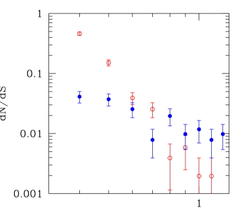
Figure 4: Comparison of the differential counts of “starburst-dominated” ($F_{8\mu\rm m}/F_{24\mu\rm m}<0.1$; open (red) circles) vs “AGN-dominated” ($F_{8\mu\rm m}/F_{24\mu\rm m}>0.1$; filled (blue) circles) galaxies in the $F_{24\mu\rm m}\geq 0.35\,$ sample of sources fainter than $R=25.5$. Counts refer to $\Delta F_{24\mu\rm m}=0.1\,$ mJy bins and are normalized to the total number of objects (510) in the overlapping MIPS-IRAC region.

3.2 Definition of the Sample

The arguments presented throughout this Section show that optically faint, 24$\,\mu\rm m$-selected objects typically identify star-forming galaxies in the redshift interval $1.6\mathrel{\hbox to0.0pt{\lower 3.0pt\hbox{$\sim$}\hss}\raise 2.0pt\hbox{$<$}}z\mathrel{\hbox to0.0pt{\lower 3.0pt\hbox{$\sim$}\hss}\raise 2.0pt\hbox{$<$}}2.7$.

There are 793 $R>25.5$ MIPS galaxies with 24$\,\mu$m fluxes brighter than 0.35 mJy in the area of approximately 3.97 square degrees ($257.25^{\circ}\mathrel{\hbox to0.0pt{\lower 3.0pt\hbox{$\sim$}\hss}\raise 2.0pt\hbox{$<$}}\hbox{RA}(2000)\mathrel{\hbox to0.0pt{\lower 3.0pt\hbox{$\sim$}\hss}\raise 2.0pt\hbox{$<$}}261.75^{\circ}$; 58.6^∘ $\mathrel{\hbox to0.0pt{\lower 3.0pt\hbox{$\sim$}\hss}\raise 2.0pt\hbox{$<$}}\hbox{Dec}\mathrel{\hbox to0.0pt{\lower 3.0pt\hbox{$\sim$}\hss}\raise 2.0pt\hbox{$<$}}$ 60.35^∘) covered by KPNO data (cutting out the irregular regions close to the borders of the 24$\mu\rm m$ field). This region encloses the 2.85 square degrees where also 8$\,\mu$m data is available. The sources selected in the above fashion correspond to 7.4% of the total number of objects (10,693) brighter than $F_{24\mu\rm m}=0.35\,$mJy found in the same area and constitute the sample which will be used in the following statistical analyses.

It is worth noting that, while the adopted 24 $\mu$m limit ensures completeness for what concerns the mid-IR selection of the sample, the optical $R>25.5$ cut is somewhat arbitrary. In fact, the studies presented in § 3.3 find sources in the $1.6\mathrel{\hbox to0.0pt{\lower 3.0pt\hbox{$\sim$}\hss}\raise 2.0pt\hbox{$<$}}z\mathrel{\hbox to0.0pt{\lower 3.0pt\hbox{$\sim$}\hss}\raise 2.0pt\hbox{$<$}}2.7$ redshift range having magnitudes brighter than our chosen value. On the other hand, some of the sources with $R\sim 24$ observed by the above authors turned out to have lower redshifts. One therefore has that a cut at $R=25.5$ ensures that the overwhelming majority (if not all) of the selected objects lie in the $z\sim 2$ range, while relaxing the optical magnitude limit may lead to a contamination of the sample, while only adding a modest fraction of sources (see also § 4 below). For example, if we lower the limit to $R=24.5$ we only add 139 objects to the adopted sample, corresponding to a fractional increase of 17.5%.

While such an incompleteness in the optical selection of the MIPS sample is not expected to affect the clustering estimates as long as the redshift distribution of $R>25.5$ sources does not greatly differ in shape from that of all galaxies belonging to the same population and endowed with mid-IR fluxes $F_{24\mu\rm m}\geq 0.35\,$mJy, the same does not hold when considering the space density of such sources; in this case, the quantity quoted in § 4 will have to be considered as a mere lower limit.

4 Clustering Properties

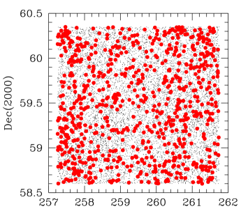
Figure 5: Sky distribution of the 793 optically faint ($R>25.5$) sources in the $F_{24\mu\rm m}\geq 0.35$ mJy MIPS sample found within the area of 3.97 square degrees covered by KPNO data (red filled circles; see text for details). The distribution of all the 24$\mu$m sources brighter than the same flux limit and enclosed in the same region of the sky is also shown for comparison (small black dots).

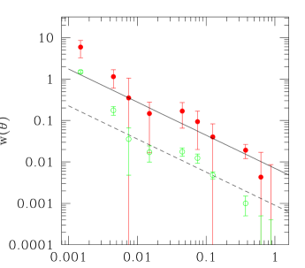
Figure 6: Angular correlation function $w(\theta)$ for $R>25.5$ sources (filled circles) and for the whole $F_{24\mu\rm m}\geq 0.35$ mJy MIPS sample (open circles). The solid and the dashed lines show the best power-law fits to the data.

A mere visual inspection of the sky distribution of the $24\,\mu$m sources with $R>25.5$ which identify the sample presented in § 3.4 (filled circles in Fig. 5), indicates that these objects are strongly clustered, much more than the sources in the full $F_{24\mu\rm m}\geq 0.35$ mJy First Look Survey (small dots).

The standard way to quantify the clustering properties of a particular class of sources of unknown distance is by means of the angular two-point correlation function $w(\theta)$ which measures the excess probability of finding a pair in the two solid angle elements $d\Omega_{1}$ and $d\Omega_{2}$ separated by an angle $\theta$. In practice, $w(\theta)$ is obtained by comparing the actual source distribution with a catalogue of randomly distributed objects subject to the same mask constraints as the real data. We chose to use the estimator (Hamilton 1993)

$$w(\theta)=4\times\frac{DD\cdot RR}{(DR)^{2}}-1,$$ (1)

in the range of scales $10^{-3}\mathrel{\hbox to0.0pt{\lower 3.0pt\hbox{$\sim$}\hss}\raise 2.0pt\hbox{$<$}}\theta\mathrel{\hbox to0.0pt{\lower 3.0pt\hbox{$\sim$}\hss}\raise 2.0pt\hbox{$<$}}1$ degrees. $DD$, $RR$ and $DR$ are the number of data-data, random-random and data-random pairs separated by a distance $\theta$. The random catalogue was generated with twenty times as many objects as the real data set, and the angular distribution of its sources was modulated according to the MIPS coverage map, so that the instrumental window function did not affect the measured clustering.

The resulting angular correlation function $w(\theta)$ for the obscured ($R>25.5$), $F_{24\mu\rm m}\geq 0.35$ mJy sources is shown by the filled circles in Fig. 6. The errors have been computed as:

$$\delta w(\theta)={1+w(\theta)\over\sqrt{DD}}.$$ (2)

Since the distributions are clustered, this (Poisson) estimate for the errors only provides a lower limit to the real uncertainties. However, it can be shown that over the considered range of angular scales this estimate is close to those obtained from bootstrap resampling (e.g. Willumsen, Freudling & Da Costa, 1997). On the other hand, the above estimate does not take into account the uncertainties on the sample selection, which we are unable to quantify but may be substantial. We tentatively allow for them by doubling the Poisson errors in the following analysis and in the Figures. The above analysis was repeated by using the Landy & Szalay (1993) estimator, and we found virtually identical results.

We have also investigated the possibility that the clustering properties of high-$z$ starburst galaxies are contaminated by obscured AGNs (see § 3.2), which may cluster differently. However, removing candidate AGNs, i.e. objects with $F_{8\mu\rm m}/F_{24\mu\rm m}>0.1$ (or alternatively $F_{24\mu\rm m}\mathrel{\hbox to0.0pt{\lower 3.0pt\hbox{$\sim$}\hss}\raise 2.0pt\hbox{$>$}}0.8\,$mJy) which make up for $\sim$20 per cent of the total sample, leaves the angular correlation function essentially unaffected, indicating that AGN-powered sources have clustering properties similar to those of starbursts.

On the other hand, if we somewhat relax the optical magnitude limit, e.g. we decrease it from $R>25.5$ to $R>24.5$, the estimated $w(\theta)$ becomes significantly noisier, even though the fraction of added sources is only 17.5% of the original sample (similar to that of “AGNs”), suggesting that a substantial portion of optically brighter, $F_{24\mu\rm m}\geq 0.35$ sources are at lower redshifts. Including still optically brighter sources, the angular correlation function rapidly decreases, approaching that obtained for the whole $24\,\mu$m-selected sample (open circles in Fig. 6; in this case the associated errors simply correspond to 1$\sigma$).

If we adopt the usual power-law form,

$$w(\theta)=A\theta^{(1-\gamma)},$$ (3)

the parameters $A$ and $\gamma$ can be estimated via a least-squares fit to the data. However, given the large errors on $w$, we choose to fix $\gamma$ to the standard value $\gamma=1.8$. We then obtain $A=(7\pm 2)\times 10^{-3}$ (solid line in Fig. 6); the point on the top left-hand corner has not been considered in our analysis because it corresponds to an angular scale close to the resolution of the instrument and therefore, despite the accuracy of the deblending technique applied to produce the original MIPS catalogue, it may be affected by source confusion.

The amplitude $A$ is about three times higher than that derived by Fang et al. (2004) for a sample of IRAC galaxies selected at 8$\mu$m ($A\sim 2.34\cdot 10^{-3}$), and about eight times higher than that obtained for the whole $F_{24\mu\rm m}\geq 0.35$ mJy MIPS dataset ($A=(9\pm 2)\cdot 10^{-4}$, dashed line in Fig. 6).

The angular correlation function is related to the spatial one, $\xi(r,z)$, by the relativistic Limber equation (Peebles, 1980):

$$w(\theta)=2\>\frac{\int_{0}^{\infty}\int_{0}^{\infty}F^{-2}(x)x^{4}\Phi^{2}(x)\xi(r,z)dx\>du}{\left[\int_{0}^{\infty}F^{-1}(x)x^{2}\Phi(x)dx\right]^{2}},$$ (4)

where $x$ is the comoving coordinate, $F(x)$ gives the correction for curvature, and the selection function $\Phi(x)$ satisfies the relation

$${\cal N}=\int_{0}^{\infty}\Phi(x)F^{-1}(x)x^{2}dx=\frac{1}{\Omega_{s}}\int_{0}^{\infty}N(z)dz,$$ (5)

in which $\cal N$ is the mean surface density, $\Omega_{s}$ is the solid angle covered by the survey, and $N(z)$ is the number of sources within the shell ($z,z+dz$).

If we make the simple assumption, consistent with the photometric and spectroscopic information summarized in § 3, that $N(z)$ is constant in the range $1.6\mathrel{\hbox to0.0pt{\lower 3.0pt\hbox{$\sim$}\hss}\raise 2.0pt\hbox{$<$}}z\mathrel{\hbox to0.0pt{\lower 3.0pt\hbox{$\sim$}\hss}\raise 2.0pt\hbox{$<$}}2.7$ and adopt a spatial correlation function of the form $\xi(r,z)=(r/r_{0})^{-1.8}$, independent of redshift (in comoving coordinates) in the considered interval, we obtain, for the adopted cosmology, $r_{0}(z=1.6-2.7)=14.0_{-2.4}^{+2.1}$ Mpc. The clustering radius increases (decreases) if we broaden (narrow) the redshift range. If we instead adopt the redshift distribution predicted by the model of Granato et al. (2004; see § 6) we get: $r_{0}(z=1.6-2.7)=15.2_{-2.6}^{+2.3}$ Mpc. Note that the assumption of a redshift independent comoving clustering radius is borne out by observational estimates for optical quasars (Porciani et al. 2004; Croom et al. 2005) which – according to the Granato et al. (2004) model – correspond to a later evolutionary phase of the AGNs hosted by $24\,\mu$m sources.

The above value of $r_{0}$ is in good agreement with the estimates obtained in the case of ultra-luminous infrared galaxies over $1.5<z<3$ (Farrah et al. 2006a,b), and also matches that found by Magliocchetti & Maddox (1999) in the analysis of the clustering properties of galaxies in the Hubble Deep Field North selected in the same redshift range. Massive star-forming galaxies at $z\sim 2$ thus appear to be amongst the most strongly clustered sources in the Universe. Locally, their clustering properties find a counterpart in those exhibited by radio sources (see e.g. Magliocchetti et al. 2004) and are only second to those of rich clusters of galaxies (e.g. Guzzo et al. 2000). The implications of this result will be investigated in the next Sections.

Under the assumption of a uniform redshift distribution in the range $1.6\mathrel{\hbox to0.0pt{\lower 3.0pt\hbox{$\sim$}\hss}\raise 2.0pt\hbox{$<$}}z\mathrel{\hbox to0.0pt{\lower 3.0pt\hbox{$\sim$}\hss}\raise 2.0pt\hbox{$<$}}2.7$ and for the adopted cosmology, the mean comoving space density of sources with $R>25.5$ and $F_{24\mu\rm m}\geq 0.35\,$mJy is:

$$\bar{n}_{\rm obs}(1.6<z<2.7)\sim 1.5\cdot 10^{-5}\ {\rm Mpc}^{-3}.$$ (6)

5 The Halo Occupation Number (HON)

A closer look to Fig. 6 shows that a simple power-law provides a good fit for the measured $w(\theta)$ only over the range $0.007^{\circ}\mathrel{\hbox to0.0pt{\lower 3.0pt\hbox{$\sim$}\hss}\raise 2.0pt\hbox{$<$}}\theta\mathrel{\hbox to0.0pt{\lower 3.0pt\hbox{$\sim$}\hss}\raise 2.0pt\hbox{$<$}}0.5^{\circ}$. Even though masked by large error bars, a hint of a steepening can in fact be discerned on the smallest angular scales and may also be present at the largest angles probed by our analysis. The small-scale steepening is intimately related to the way the sources under exam occupy their dark matter haloes, issue which will be dealt with throughout this Section via the so-called Halo Occupation Scenario, while the steepening on large angular scales is most likely due to the high redshift of these sources ($0.5^{\circ}$ in the adopted cosmology and for a redshift $z=2$ correspond to a scale of $\sim 45$ Mpc above which the real-space correlation function rapidly approaches zero).

5.1 Setting up the formalism

The halo occupation function is defined as the probability distribution of the number of galaxies brighter than some luminosity threshold hosted by a virialized halo of given mass. Within this framework, it is possible to show (see e.g. Peacock & Smith 2000 and Scoccimarro et al. 2001) that the distribution of galaxies within their dark matter haloes determines the galaxy-galaxy clustering on small scales. Since the distribution of sources within their haloes in general depends on the efficiency of galaxy formation, clustering measurements can provide important insights on the physics of those objects producing the signal. This approach has been successfully applied in the past few years to a number of cases, from local galaxies (Magliocchetti & Porciani 2003; Zehavi et al. 2004) to higher redshift sources such as COMBO 17 and Lyman Break galaxies (e.g. Phleps et al. 2005; Hamana et al. 2003; Ouchi et al. 2005) and quasars (Porciani, Magliocchetti & Norberg 2004).

Our analysis follows the approach adopted by Magliocchetti & Porciani (2003), which is in turn based on the work by Scherrer & Bertschinger (1991) and Scoccimarro et al. (2001). The basic quantity here is the halo occupation distribution function $P_{N}(M)$ which gives the probability of finding $N$ galaxies within a single halo as a function of the halo mass $M$. Given the halo mass function $n(M)$ (number density of dark matter haloes per unit comoving volume and $\log_{10}(M)$), the mean value of the halo occupation distribution $N(M)\equiv\langle N\rangle(M)=\sum_{N}N\,P_{N}(M)$ (which, from now on, we will call the halo occupation number) completely determines the mean comoving number density of galaxies in the desired redshift range:

$$n_{\rm gal}=\int n(M)\,N(M)\,dM\;.$$ (7)

Relations, analogous to eq. (7) and involving higher-order moments of $P_{N}(M)$, can be used to derive the clustering properties in the framework of the halo model. For instance, the 2-point correlation function can be written as the sum of two terms

$$\xi(r)=\xi^{1h}(r)+\xi^{2h}(r)\;.$$ (8)

The function $\xi^{1h}$, which accounts for pairs of galaxies residing within the same halo, depends on the second factorial moment of the halo occupation distribution $\sigma(M)=\langle N(N-1)\rangle(M)$ and on the spatial distribution of galaxies within their host haloes $\rho({\bf x}|M)$, normalized in such a way that $\int_{0}^{r^{\rm vir}}\rho({\bf y}|M)d^{3}y=1$ where $r^{\rm vir}$ is the virial radius which is assumed to mark the outer boundary of the halo:

$$\xi^{1h}(r)=\!\!\int\frac{n(M)\,\sigma(M)}{n_{\rm gal}^{2}}\,dM\int\rho({\bf x}|M)\,\rho({\bf x}+{\bf r}|M)\,d^{3}x.$$ (9)

On the other hand, the term $\xi^{2h}$, which takes into account the contribution to the correlation function coming from galaxies in different haloes, depends on both $N(M)$ and $\rho({\bf x}|M)$ as follows

$$\xi^{2h}(r)\!\!\! = \!\!\!\!\!\int\frac{n(M_{1})\,N(M_{1})}{n_{\rm gal}}\,dM_{1}\int\frac{n(M_{2})\,N(M_{2})}{{n_{\rm gal}}}\,dM_{2}$$ (10)

$$\times \!\!\!\!\!\int\!\!\rho({\bf x}_{1}|M_{1})\,\rho({\bf x}_{2}|M_{2})\,\xi({\bf r}_{12}|M_{1},M_{2})\,d^{3}r_{1}\,d^{3}r_{2},$$

where $\xi(r|M_{1},M_{2})$ is the cross-correlation function of haloes of mass $M_{1}$ and $M_{2}$, ${\bf x}_{i}$ denotes the distance from the centre of each halo, and ${\bf r}_{12}$ is the separation between the haloes.

For separations smaller than the virial radius of the typical galaxy host halo, the 1-halo term dominates the correlation function, while the 2-halo contribution is the most important one on larger scales. In this latter regime $\xi(r|M_{1},M_{2})$ is proportional to the mass autocorrelation function, i.e. $\xi(r|M_{1},M_{2})\simeq b(M_{1})\,b(M_{2})\,\xi_{dm}(r)$, where $b(M)$ is the linear bias factor of haloes of mass $M$. Note that all the different quantities introduced in this Section depend on the redshift $z$ even though we have not made it explicit in the equations.

In order to use the halo model to study the galaxy clustering, one has to specify a number of functions describing the statistical properties of the population of dark matter haloes. In general, these have either been obtained analytically and calibrated against N-body simulations, or directly extracted from numerical experiments.

For the mass function and the linear bias factor of dark matter haloes we adopt here the model by Sheth & Tormen (1999), while we write the two-point correlation function of dark-matter haloes as (see e.g. Porciani & Giavalisco 2002; Magliocchetti & Porciani 2003)

$$\xi(r|M_{1},M_{2})\!\!=\!\!\left\{\begin{array}[]{ll}\!\!\!\!\xi_{dm}(r)b_{1}(M_{1})b_{2}(M_{2})&\!\!\!\!{\rm if}\;r\geq r^{\rm vir}_{1}\!\!+r^{\rm vir}_{2}\\ \!\!\!\!-1&{\rm otherwise},\end{array}\right.$$ (13)

where the mass autocorrelation function, $\xi_{dm}(r)$, is computed with the method of Peacock & Dodds (1996) and the above expression takes into account the spatial exclusion between haloes (i.e. two haloes cannot occupy the same volume). We will also assume that the distribution of galaxies within their haloes traces that of the dark matter and we adopt for $\rho({\bf x}|M)$ a Navarro, Frenk & White (1997) profile with a concentration parameter obtained from eqs. (9) and (13) of Bullock et al. (2001). In fact, Magliocchetti & Porciani (2003) showed that NFW profiles are well suited to describe the correlation function of local 2dF galaxies. We note however that the uncertainties associated to our estimates of $w(\theta)$ do not allow us to discriminate between different forms for $\rho({\bf x}|M)$ as long as they are sensible ones (e.g. profiles of the form $\rho\propto r^{-\beta}$ with $2\mathrel{\hbox to0.0pt{\lower 3.0pt\hbox{$\sim$}\hss}\raise 2.0pt\hbox{$<$}}\beta\mathrel{\hbox to0.0pt{\lower 3.0pt\hbox{$\sim$}\hss}\raise 2.0pt\hbox{$<$}}3$, $\beta=2$ corresponding to the singular isothermal sphere case).

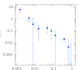
Figure 7: Best fit to the observed angular correlation function $w(\theta)$ of our sources, in the HON framework for $\alpha=0.2$, $M_{\rm min}=10^{13.4}M_{\odot}$, $\rm log_{10}(N_{0})=-0.3$. The point on the smallest angular scale has not been taken into account, because of uncertainties in source deblending.

The final key ingredient needed to describe the clustering properties of a class of galaxies is their halo occupation function $P_{N}(M)$. In the ideal case $P_{N}(M)$ is entirely specified by the knowledge of all its moments which in principle can be observationally determined by studying galaxy clustering at any order. Unfortunately this is not feasible in practice, as measures of the higher moments of the galaxy distribution get extremely noisy for $n>4$ even for local 2-dimensional catalogues (see e.g. Gaztañaga, 1995 for an analysis of the APM survey). On the other hand, the present work relies on measurements of the two-point correlation function, which only depends on the first two moments of the halo occupation function, $N(M)$ and $\sigma(M)$.

Following Porciani et al. (2004; see also Magliocchetti & Porciani 2003 and Hatton et al. 2003) we parameterize these quantities as:

$$N(M)=\left\{\begin{array}[]{ll}N_{0}(M/M_{\rm min})^{\alpha}&\rm{if}\ M\geq M_{\rm min}\\ 0&\rm{if}\ M<M_{\rm min}\end{array}\right.$$ (16)

and

$$\sigma(M)=\beta(M)^{2}N(M),$$ (17)

where $\beta(M)=0,{\rm log}(M/M_{\rm min})/{\rm log}(M/M_{0}),1$, respectively for $N(M)=0$, $N(M)<1$ and $N(M)\geq 1$. The operational definition of $M_{0}$ is such that $N(M_{0})=1$ (see e.g. Porciani et al. 2004), while $M_{\rm min}$ is the minimum mass of a halo able to host a source of the kind under consideration. More and more massive haloes are expected to host more and more galaxies, justifying the assumption of a power-law shape for the halo occupation number. As already pointed out in Porciani et al. (2004), eq. (16) is more general than the commonly used $N(M)=(M/M_{0})^{\alpha}$ which, for $\alpha=0$, automatically implies $N(M)=1$ at any $M>M_{0}$.

As for the variance $\sigma(M)$, we note that the high-mass value for $\beta(M)$ simply reflects the Poisson statistics, while the functional form at intermediate masses (chosen to fit the results from semi-analytical models – see e.g. Sheth & Diaferio 2001; Berlind & Weinberg 2002 – and hydrodynamical simulations – Berlind et al. 2003) describes the (strongly) sub-Poissonian regime. We assume the various quantities describing the HON not to vary in the considered redshift range. Although a simplification, this choice is partially justified by the results obtained for other extragalactic sources sampling the same redshift range of our dataset (e.g. quasars, see Porciani et al. 2004), which indeed show the relevant parameters associated to $N(M)$ to stay constant with look-back time.

Figure 8: Average number of MIR-bright ($F_{24\mu\rm m}\geq 0.35$ mJy), optically faint ($R>25.5$), galaxies per dark matter halo of specified mass $M$ in the redshift range $z\simeq[1.6-2.7]$. The solid line corresponds to the best-fit values of eq. (15), while the dashed lines correspond to cases with $\Delta\chi^{2}=1$ (see text).

5.2 Results

In the application of the HON formalism to the present sample we allowed the parameters of eq. (16) to vary within the following ranges:

$$0\leq\alpha\leq 2$$

$$10^{11}\;M_{\odot}\leq M_{{\rm min}}\leq 10^{14}\;M_{\odot}$$ (18)

$$-2\leq\log_{10}(N_{0})\leq 1\ .$$

Values for these parameters have been determined through a minimum $\chi^{2}$ technique by fitting the observed $w(\theta)$ (except for the smallest angular scale point, cfr. § 4). The angular correlation function was computed from eq. (4), with $\xi(r)$ given by eq. (8) and the redshift distribution yielded by the Granato et al. (2004) model (see § 6).

We find that the best fit to the $w(\theta)$ alone is obtained for:

$$\alpha=0.2^{+0.7}_{-0.2}\;\;\;\;\;\;\;\;\;\;\;\;\;\;\;\;\;\;\;\;\;\;\;\;\;$$

$${\log}_{10}(M_{\rm min}/M_{\odot})=13.5^{+0.2}_{-0.4}\;\;,$$ (19)

$${\log}_{10}(N_{0})=-0.3^{+0.2}_{-1.7}\;\;\;\;\;\;\;\;\;\;$$

where the quoted errors correspond to $\Delta\chi^{2}=1$. We note however that the sampled correlation function bins are not completely independent, so that the error estimate is only indicative.

The parameters are correlated with each other. In particular, higher values for $M_{\rm min}$ correspond to lower values of $\alpha$ (see Fig. 8). Furthermore, as $N_{0}$ is always found to be less than 1 and the index $\alpha$ is rather flat, on average there is less than one of such star-forming galaxies per dark matter halo (sub-Poissonian regime) except at the highest/cluster-like mass scales.

It may be noted that the data on $w(\theta)$ can only effectively constrain $M_{\rm min}$, while allowing for relatively broad ranges in the case of $N_{0}$ and $\alpha$. This can be easily understood since, for typical halo masses $>>M^{*}$ the halo bias function $b(M)$ is a steep function of $M$, so that even small variations of $M_{\rm min}$ result in large variations of the predicted $w(\theta)$ on intermediate-to-large angular scales. On the other hand, $N_{0}$ can only be constrained by data on small angular scales (one-halo regime) via the theoretical variance $\sigma(M)$. But the one-halo regime is represented by just one data point and furthermore, as long as the regime is sub-Poissonian, the predicted one-halo correlation function is only mildly dependent on this quantity.

Additional constraints on the three parameters characterizing the HON [eq. (16)] can be obtained from the estimated comoving number density of our sources. In fact, any HON model must simultaneously be able to reproduce both the first and second moment of the galaxy distribution, i.e. both the clustering properties and the observed number density of sources in a specified sample. As discussed in § 4, the estimate in eq. (6) is expected to provide a lower limit to the number density of high-redshift star-forming galaxies with $F_{24\mu\rm m}\geq 0.35$, although with a substantial uncertainty, mostly related to our poor knowledge of the redshift distribution. If we then require $n_{\rm gal}$ in eq. (7) to be $\geq 6\cdot 10^{-6}\ {\rm Mpc}^{-3}$ (i.e. allow for an uncertainty of a factor of 2.5) the permitted ranges for the parameters narrow down becoming:

$$\alpha=0.2^{+0.4}_{-0.1}\;\;\;\;\;\;\;\;\;\;\;\;\;\;\;\;\;\;\;\;\;\;\;\;\;$$

$${\log}_{10}(M_{\rm min}/M_{\odot})=13.4^{+0.1}_{-0.3}$$ (20)

$${\log}_{10}(N_{0})=-0.3^{+0.2}_{-0.6}\ ,\;\;\;\;\;\;\;\;\;\;$$

which are the best-fit values for the HON [eq. (16)] satisfying both the clustering and the number density requirement. We note that, while as expected the range for $M_{\rm min}$ is basically unaffected, the constraint on $n_{\rm gal}$ greatly shrinks the allowed region for $N_{0}$ by cutting all those values which would have produced too few sources. The above best-fit values do not change significantly if instead of the $N(z)$ deriving from the Granato et al. (2004) model we use the flat redshift distribution introduced in § 3; in this case we get $\alpha=0.3^{+0.3}_{-0.2}$; ${\log}_{10}(M_{\rm min}/M_{\odot})=13.3^{+0.1}_{-0.2}$; ${\log}_{10}(N_{0})=-0.4^{+0.3}_{-0.3}$.

The theoretical angular correlation function corresponding to the above best-fit HON parameters is compared to the data in Fig. 7. The model correctly describes both the overall amplitude of $w(\theta$) and the rise on angular scales $\mathrel{\hbox to0.0pt{\lower 3.0pt\hbox{$\sim$}\hss}\raise 2.0pt\hbox{$<$}}10^{-2}$ deg determined by the one-halo regime. The corresponding Halo Occupation Number of high-redshift star-forming galaxies is presented in Fig. 8, which shows that the sources under exam are always associated to very massive structures, identifiable with groups-to-clusters of galaxies. As it is also possible to notice, such galaxies are reasonably common in those massive structures, with an average of $\sim 0.5-1$ object per group, where the upper value is found in correspondence of the highest masses probed by our analysis. The implications of these results will be investigated in the next Section, when discussing the nature of optically faint objects as selected at 24$\mu$m.

Figure 9: Number of $24\,\mu$m sources fainter than $R=25.5$ (filled squares) and of all 24$\mu$m MIPS sources counted, in $\Delta F_{24\mu\rm m}=0.1\,$mJy bins, in the $3.97\,\hbox{deg}^{2}$ area covered by KPNO data. The lower panel represents the ratio between the above quantities as a function of the 24$\mu$m flux, while the dashed line in the top panel shows the predictions by Silva et al. (2004; 2005) for high-$z$ proto-spheroidal galaxies.

Figure 10: Redshift distribution of dusty proto-spheroidals with fluxes $F_{24\mu\rm{m}}\geq 0.35\,$mJy, normalized to unity, obtained following Silva et al. (2004; 2005).

6 Nature of the sources

Before the Spitzer survey data became available, Silva et al. (2004; 2005) worked out detailed predictions for the counts and the redshift distributions of IR sources. In particular they predicted that for $F_{24\rm\mu m}\mathrel{\hbox to0.0pt{\lower 3.0pt\hbox{$\sim$}\hss}\raise 2.0pt\hbox{$>$}}0.35$ mJy, MIPS surveys would have comprised a small, but significant (8–10%) fraction of objects in the redshift range $\sim 1.5--2.6$ (with a tail extending up to $z\mathrel{\hbox to0.0pt{\lower 3.0pt\hbox{$\sim$}\hss}\raise 2.0pt\hbox{$>$}}3$; cfr. their Figure 27). At the flux limit ($F_{24\rm\mu m}\geq 83\,\mu$Jy) of the MIPS survey of the Chandra Deep Field South (Papovich et al. 1984), Silva et al. (2004; 2005) predicted a surface density of proto-spheroids at $z\geq 1.5$ of $\simeq 1\,\hbox{arcmin}^{-2}$, i.e. amounting to $\simeq 22\%$ of the observed total surface density. This prediction was at variance with those of reference phenomenological models which, for $F_{24\mu\rm m}\geq 83\,\mu$Jy, yielded (see Figure 2 of Pérez-González et al. 2005 and Figure 6 of Caputi et al. 2006) either very few (Chary et al. 2004) or almost 50% (Lagache et al. 2004) sources at $z\mathrel{\hbox to0.0pt{\lower 3.0pt\hbox{$\sim$}\hss}\raise 2.0pt\hbox{$>$}}1.5$. The redshift distribution by Pérez-González et al. (2005) for $F_{24\mu\rm m}\geq 83\,\mu$Jy, based primarily on photometric redshifts for starburst templates, has about 24% of sources at $z\geq 1.5$. This result was recently confirmed, within the errors, by the work of Caputi et al. (2006) who found $\simeq 28\%$ of sources to lie in that $z$ range.

The basic difference between the work of Silva et al. (2004; 2005) and that of the other quoted models is that, while Chary et al. (2004) and Lagache et al. (2004) adopt a purely empirical/phenomenological approach to describe the high redshift population of galaxies selected at 24$\mu$m (by e.g. evolving the local luminosity function in luminosity and/or density), Silva et al. (2004; 2005) consider a more physically grounded picture. In fact, according to Silva et al. (2004; 2005) the $z\mathrel{\hbox to0.0pt{\lower 3.0pt\hbox{$\sim$}\hss}\raise 2.0pt\hbox{$>$}}1.5$ population corresponds to massive proto-spheroidal galaxies in the process of forming most of their stars in a gigantic starburst, whose evolution is described by the physical model of Granato et al. (2004). This population is not represented in the local far-IR luminosity function, since local massive spheroids are essentially dust-free. We refer the interested reader to the Granato et al. (2004) paper for a full account of the physical justification and a detailed description of the model. Here we provide a short summary of its main features, focusing on the aspects which are relevant to the present discussion.

6.1 Overview of the Granato et al. (2004) model

The model adopts the standard hierarchical clustering framework for the formation of dark matter haloes. It focuses on the redshift range $z\ga 1.5$, where a good approximation of the halo formation rates is provided by the positive term in the cosmic time derivative of the cosmological mass function (e.g., Haehnelt & Rees 1993; Sasaki 1994). The simulations by Wechsler et al. (2002), and Zhao et al. (2003a,b) show that the growth of a halo occurs in two different phases: a first regime of fast accretion in which the potential well is built up by the sudden mergers of many clumps of comparable mass; and a second regime of slow accretion in which mass is added in the outskirts of the halo, without affecting the central region where the galactic structure resides. This means that, even at high redshift, once created the haloes harboring a massive elliptical galaxy are rarely destroyed and get incorporated within groups and clusters of galaxies.

The physics governing the evolution of the baryons is much more complex. The main features of the model can be summarized as follows (see Granato et al. 2004, Cirasuolo et al. 2005, Lapi et al. 2006). During or soon after the formation of the host dark matter halo, the baryons falling into the newly created potential well are shock-heated to the virial temperature. The hot gas is (moderately) clumpy and cools quickly especially in the denser central regions, triggering a strong burst of star formation. The radiation drag due to starlight acts on the gas clouds, reducing their angular momentum. As a consequence, a fraction of the cool gas can fall into a reservoir around the central super-massive black hole, and eventually accretes onto it by viscous dissipation, powering the nuclear activity. The energy fed back to the gas by supernova explosions and black hole activity regulates the ongoing star formation and the black hole growth.

Initially, the cooling is rapid and the star formation is very high; thus the radiation drag is efficient in accumulating mass into the reservoir. The black hole starts growing from an initial seed with mass $\sim 10^{2}\,M_{\odot}$ already in place at the galactic center. Since there is plenty of material in this phase, the accretion is Eddington (or moderately super-Eddington) limited (e.g., Small & Blandford 1992; Blandford 2004). This regime goes on until the energy feedback from the black hole is strong enough to unbind the gas from the potential well, a condition occurring around the peak of the accretion curve. Subsequently, the star formation rate drops substantially, the radiation drag becomes inefficient, the storage of matter in the reservoir and the accretion onto the black hole decrease by a large factor. The drop is very pronounced for massive haloes, $M_{\mathrm{vir}}\ga 10^{12}\,M_{\odot}$, while for smaller masses a smoother declining phase can continue for several Gyrs, and the black hole and stellar masses can further increase by a substantial factor.

Before the peak, radiation is highly obscured by the surrounding dust. In fact, these proto-galaxies are extremely faint in the rest frame UV/optical/near-IR and are more easily selected at far-IR to mm wavelengths. Nuclear emission is heavily obscured too, but since absorption significantly decreases with increasing X-ray energy of the photons, this may be detected in hard X-ray bands (Alexander et al. 2005; Borys et al. 2005; Granato et al. 2006). The mid-IR region may also be particularly well suited to detect such an emission, because the dust temperature in the nuclear torus, hotter than that of the interstellar medium, makes this component more prominent, and the optical depth is relatively low.

6.2 Model versus observations

The 24$\mu$m counts of candidate high-$z$ proto-spheroidal galaxies predicted by Silva et al. (2004; 2005) are compared, in Fig. 9, with those of MIPS sources fainter than $R=25.5$. The total 24$\mu$m counts for the MIPS sample are also shown for comparison.

The fraction of optically faint sources decreases from $\simeq 10\%$ at the lowest 24$\mu$m fluxes to less than 5% at the brightest ones. The decrement of this fraction with increasing flux is slowed down or halted above $\simeq 0.8\,$mJy, when the ‘AGN’ contribution takes over.

The dashed line in Fig. 9 represents the predictions by Silva et al. (2004; 2005), based on the Granato et al. (2004) model, for the counts at 24$\mu$m of dusty proto-spheroidals undergoing intense star formation. It must be noted that Silva et al. adopted a highly simplified description of the very complex source spectra in the relevant rest-frame frequency range, where strong emission and absorption features present a broad distribution of equivalent widths. Also, although the model explicitly predicts a significant nuclear activity with an exponential growth of the central black hole mass during the active star forming phase, nuclear emission was neglected in the calculations by Silva et al. (2004; 2005). Thus, an accurate match of the observed counts cannot be expected. Still, the observed counts of optically faint sources are remarkably close to the predictions, suggesting that objects in the present sample are high-$z$ proto-spheroidal galaxies. The redshift distribution of those sources brighter than 0.35 mJy at 24$\mu$m (Fig. 10), computed by following Silva et al. (2004; 2005), matches the redshift range estimated in the previous sections on the basis of photometric and spectroscopic evidences.

Following again Silva et al. (2004; 2005) we obtain that $\sim 5\%$ of proto-spheroidal galaxies with $F_{24\mu{\rm m}}\geq 0.35\,$mJy have $850\,\mu$m flux $\geq 10\,$mJy, consistent with the fact that none of the four sources in our sample lying in the 151 arcmin² area surveyed with SCUBA by Sawicki & Webb (2005) to the above $850\,\mu$m flux limit was detected. The model predicts most (80–90%) of proto-spheroidal galaxies with $F_{24\mu{\rm m}}\geq 0.35$ mJy to have $F_{850\mu{\rm m}}\geq 1$ mJy, but these are only a small fraction (2–4%) of ${850\mu{\rm m}}$ sources at this flux limit.

We note that such a spread in the predicted $850\,\mu$m fluxes reflects the spread in star formation rates (SFRs). The $\sim 5\%$ of proto-spheroidal galaxies selected at 24 $\mu$m with $F_{850\mu{\rm m}}\geq 10\,$mJy are predicted to have $\hbox{SFR}\mathrel{\hbox to0.0pt{\lower 3.0pt\hbox{$\sim$}\hss}\raise 2.0pt\hbox{$>$}}1000\,M_{\odot}\,\hbox{yr}^{-1}$, while about 20–30% of the sample sources should have $\hbox{SFR}\mathrel{\hbox to0.0pt{\lower 3.0pt\hbox{$\sim$}\hss}\raise 2.0pt\hbox{$>$}}500\,M_{\odot}\,\hbox{yr}^{-1}$, and about 90% are characterized by $\hbox{SFR}\mathrel{\hbox to0.0pt{\lower 3.0pt\hbox{$\sim$}\hss}\raise 2.0pt\hbox{$>$}}100\,M_{\odot}\,\hbox{yr}^{-1}$. Most of the sources have $\hbox{SFR}\sim\hbox{few}\times 100\,M_{\odot}\,\hbox{yr}^{-1}$.

The median halo mass, estimated from the model, is $\log_{10}(M_{\rm vir}/M_{\odot})\simeq 12.7$. The corresponding peak SFR ranges from 550 to $\sim 800\,M_{\odot}\,\hbox{yr}^{-1}$ for virialization redshifts ranging from 3 to 4, i.e. is substantially higher than the typical SFRs of the $24\,\mu$m sources. This means that, according to the Granato et al. (2004) model, the $24\,\mu$m selection preferentially identifies sources in the phase when the effect of feedbacks has begun to damp the SFR, at the same time decreasing the optical depth, which, at earlier times, is very high even at rest-frame mid-IR wavelengths. In this phase the active nucleus is approaching its maximum luminosity and can therefore show up at relatively bright flux densities for a relatively short time, while the starburst luminosity is far higher than that of the AGN over most of its lifetime.

Also, the estimated halo mass is substantially lower than that accounting for the clustering properties (cfr. § 5). According to the model, this difference is to be expected since the starburst phase of these haloes has a lifetime which is shorter than the Hubble time by a factor of $\sim 5$ at $z\sim 2$. This means that starburst galaxies work as beacons signalling the presence of larger haloes, typically hosting $\sim 5$ galactic haloes with $\log_{10}(M_{\rm vir}/M_{\odot})\simeq 12.7$, out of which only one is seen at $24\,\mu$m.

7 Conclusions

We have found that optically very faint ($R>25.5$) galaxies selected at $24\,\mu$m ($F_{24\mu{\rm m}}\geq 0.35\,$mJy) are very strongly clustered. Their two-point angular correlation function has an amplitude which is about 8 times higher than that found for the full $F_{24\mu{\rm m}}\geq 0.35\,$mJy sample, and about 3 times higher than the one estimated by Fang et al. (2004) for a sample selected at $8\,\mu$m. Radio, sub-mm, mid-IR, and optical photometric data converge in indicating that these sources are very luminous star-forming galaxies set at redshifts $1.6\mathrel{\hbox to0.0pt{\lower 3.0pt\hbox{$\sim$}\hss}\raise 2.0pt\hbox{$<$}}z\mathrel{\hbox to0.0pt{\lower 3.0pt\hbox{$\sim$}\hss}\raise 2.0pt\hbox{$<$}}3$. Spectroscopic redshifts for sources with similar photometric properties fall in the range $1.6\leq z\leq 2.7$. If sources have a relatively flat distribution in the above redshift interval, and we adopt the conventional power-law representation for the spatial two-point correlation function, $\xi(r,z)=(r/r_{0})^{-1.8}$, we obtain, for the adopted cosmology, a comoving clustering radius of $r_{0}(z=1.6-2.7)=14.0_{-2.4}^{+2.1}\,$Mpc, implying that these sources are amongst the most strongly clustered objects in the universe. This result is in good agreement with the estimates for ultra-luminous infrared galaxies over the redshift range $1.5<z<3$ obtained by Farrah et al. (2006a,b) by selecting sources with $F_{8\mu{\rm m}}\geq 0.4\,$mJy, $R>22$ and bumps in either the 4.5 or the $5.8\,\mu$m IRAC channel: $r_{0}=14.4\pm 1.99h^{-1}\,$Mpc for the $2<z<3$ sample (bump in the $5.8\,\mu$m channel) and $r_{0}=9.40\pm 2.24h^{-1}\,$Mpc for the $1.5<z<2.0$ sample (bump in the $4.5\,\mu$m channel).

The halo model provides a good fit of the observed angular correlation function for a minimum halo mass of $\simeq 10^{13.4}\,M_{\odot}$. The number density of haloes above this mass if fully consistent with that of our sources, therefore providing an independent test of the results derived from the $w(\theta)$ alone.

At rest-frame wavelengths $\sim 8\mu$m, (corresponding to the selection wavelength for the typical redshifts $z\sim 2$ of our sources) both the direct starlight and the interstellar dust emission are relatively low, so that nuclear activity can more easily show up. In fact, indications that optically faint Spitzer sources with $F_{24\mu{\rm m}}\mathrel{\hbox to0.0pt{\lower 3.0pt\hbox{$\sim$}\hss}\raise 2.0pt\hbox{$>$}}1\,$mJy are AGN dominated have been reported (Houck et al. 2005; Weedman et al. 2006). Comparing the redshift dependencies of the $8\mu{\rm m}/24\mu{\rm m}$ flux ratios corresponding to the SEDs of well-known galaxies such as Arp 220 (starburst galaxy) and of Mkn 231 (obscured AGN) we find that, over the redshift range of interest here, starburst galaxies are expected to have $F_{8\mu{\rm m}}/F_{24\mu{\rm m}}<0.1$ and AGN-dominated sources $F_{8\mu{\rm m}}/F_{24\mu{\rm m}}>0.1$. Adopting this criterion, we find that in our sample the latter sources dominate for $F_{24\mu{\rm m}}\geq 0.8\,$mJy, while starburst galaxies prevail at fainter fluxes comprising $\simeq 80\%$ of the sample. No significant difference in the clustering properties of the two sub-populations was detected.

Our optically faint sources that, as argued above, are most likely at $1.6\leq z\leq 2.7$, comprise $\simeq 7.4\%$ of the complete $F_{24\mu{\rm m}}\geq 0.35\,$mJy sample. This fraction is remarkably close to the prediction by Silva et al. (2004; 2005). These authors pointed out that the physically grounded evolutionary model for massive spheroidal galaxies by Granato et al. (2004) implies that the active star-forming phase of these objects had to show up in $24\,\mu$m MIPS surveys and estimated that they constitute $\simeq 8$–10% of all sources brighter than $F_{24\mu{\rm m}}\simeq 0.35\,$mJy and cover the redshift range 1.5–2.6 (with a tail extending up to $z\mathrel{\hbox to0.0pt{\lower 3.0pt\hbox{$\sim$}\hss}\raise 2.0pt\hbox{$>$}}3$; cfr. Figure 27 of Silva et al. 2004). At the flux limit ($83\,\mu$Jy) of the $24\,\mu$m MIPS survey of the Chandra Deep Field South, the model predicts a surface density of $\simeq 1.0\,\hbox{arcmin}^{-2}$ for sources at $z>1.5$ ($\simeq 22\%$ of the total surface density of sources brighter than that flux limit), in nice agreement with the observational determinations by Pérez-González et al. (2005) and Caputi et al. (2006), yielding fractions of 24% and 28% (corresponding to surface densities of $\simeq 1.1$–$1.3\,\hbox{arcmin}^{-2}$.

The photometric (radio, sub-mm, mid-IR, optical) properties of our sources are all consistent with their interpretation in terms of massive star-forming proto-spheroidal galaxies. The Granato et al. (2004) model features a tight connection between star-formation activity and growth of the active nucleus hosted by the galaxy. It thus naturally accounts for the indications of a dominant AGN contribution for $F_{24\mu{\rm m}}\geq 0.8\,$mJy.

According to this model, most sources have high, but not extreme, star-formation rates (SFRs), $\hbox{SFR}\sim\hbox{few}\times 100\,M_{\odot}\,\hbox{yr}^{-1}$, well below the peak SFR reached during their evolution. This is because during the most active star-forming phases the optical depth of the interstellar medium is very high even at rest-frame wavelengths of $\sim 8\mu$m. Thus, the $24\,\mu$m selection preferentially singles out sources in the phase when the effect of feedbacks has begun to damp the SFR, at the same time substantially decreasing the optical depth. In this phase, the active nucleus is approaching its maximum luminosity and shows up, for a short time, at the brightest flux levels, as is indeed observed.

The median galactic halo mass, estimated from the model, is $\log_{10}(M_{\rm vir}/M_{\odot})\simeq 12.7$, sensibly lower than that accounting for the clustering properties. This difference is due to the fact that the lifetime of the starburst phase of these haloes is shorter (by a factor $\simeq 5$) than the Hubble time, so that starburst galaxies work as beacons signalling the presence of larger haloes, typically hosting $\simeq 5$ galactic haloes with $\log_{10}(M_{\rm vir}/M_{\odot})\simeq 12.7$, out of which only one is bright enough at $24\,\mu$m to meet the observational selection.

Once we account for this lifetime effect, the comoving density of proto-spheroidal galaxies at $z\simeq 2$ matches that of $\log_{10}(M_{\rm vir}/M_{\odot})\simeq 12.7$ haloes in the same epoch, and is substantially higher than what predicted by most semi-analytic models for galaxy formation.

References

- [] Alexander D.M., Bauer, F.E., Chapman, S.C., Smail, I., Blain, A.W., Brandt, W.N., & Ivison, R.J., 2005, ApJ, 632, 736
- [\citeauthoryearArmus et al.2004] Armus L., et al., 2004, ApJS, 154, 178
- [Baugh2005] Baugh C.M., Lacey C.G. Frenk C.S., Granato G.L., Silva L., Bressan A., Benson A.J., Cole S., 2005, MNRAS, 356, 1191
- [Berlind2002] Berlind A.A., Weinberg D.H., 2002, ApJ, 575, 587
- [Berletal2003] Berlind A.A. et al., 2003, ApJ, 593, 1
- [Blain2005] Blain A.W., Chapman S.C., Smail I., Ivison R., 2005, proc. ESO workshop on ”Multiwavelength Mapping of Galaxy Formation and Evolution”, p. 94
- [] Blandford R.D., 2004, in Coevolution of Black Holes and Galaxies, ed. L.C. Ho, Cambridge Univ. Press, p. 153
- [] Borys C., Smail I., Chapman S.C., Blain A.W., Alexander D.M., Ivison R.J., 2005, ApJ, 635, 853
- [Bullock2001] Bullock J.S., Dekel A., Kolatt T.S., et al., 2001, ApJ, 555, 240
- [Bundi2005] Bundy K., et al., 2006, astro-ph/0512465
- [Caputi2006] Caputi K.I., et al. 2006, ApJ, 637, 727
- [chap2005] Chapman S.C., Blain A.W., Smail I., Ivison R.J., 2005, ApJ, 622, 772
- [\citeauthoryearCharmandaris et al.2004] Charmandaris V., et al., 2004, ApJS, 154, 142
- [\citeauthoryearChary et al.2004] Chary R., et al., 2004, ApJS, 154, 80
- [\citeauthoryearChoi et al.2006] Choi P.I., et al., 2006, ApJ, 637, 227
- [cimatti2004] Cimatti A., et al., 2004, Nature, 430, 184
- [cirasuolo2005] Cirasuolo M., Shankar F., Granato G.L., De Zotti G., Danese L., 2005, ApJ, 629, 816
- [\citeauthoryearCondon et al.2003] Condon J.J., Cotton W.D., Yin Q.F., Shupe D.L., Storrie-Lombardi L.J., Helou G., Soifer B.T., Werner M.W., 2003, AJ, 125, 2411
- [cowie1996] Cowie L.L., Songaila A., Hu E., Cohen J.G., 1996, AJ, 112, 839
- [\citeauthoryearCroom et al.2005] Croom S. M., et al., 2005, MNRAS, 356, 415
- [Eales2000] Eales S., Lilly. S., Webb T., Dunne L., Gear W., Clements D., Yun M., 2000, AJ, 120, 2244
- [\citeauthoryearEgami et al.2004] Egami E., et al., 2004, ApJS, 154, 130
- [\citeauthoryearEllis et al.1997] Ellis R.S., Smail I., Dressler A., Couch W.J., Oemler A.J., Butcher H., Sharples R.M., 1997, ApJ, 483, 582
- [] Faber S.M., et al., 2006, ApJ, submitted, astro-ph/0506044
- [fadda2004] Fadda D., Jannuzi B.T., Ford A., Storrie-Lombardi L.J., 2004, AJ, 128, 1
- [fadda062006] Fadda D. et al. 2006, astro-ph/0603488
- [fang2004] Fang F., et al., 2004, ApJS, 154, 35
- [\citeauthoryearFarrah et al.2006a] Farrah D., et al., 2006a, ApJ, 641, L17
- [\citeauthoryearFarrah et al.2006b] Farrah D., et al., 2006b, ApJ, 643, L139
- [\citeauthoryearFontana et al.2004] Fontana A., et al., 2004, A&A, 424, 23
- [\citeauthoryearFrayer et al.2004] Frayer D. T., et al., 2004, ApJS, 154, 137
- [Fuk1995] Fukugita M., Shimasaku K., Ichikawa T., 1995, PASP, 107, 945
- [Gatz1995] Gaztañaga E., 1995, MNRAS, 454, 561
- [\citeauthoryearGiallongo et al.2005] Giallongo E., Salimbeni S., Menci N., Zamorani G., Fontana A., Dickinson M., Cristiani S., Pozzetti L., 2005, ApJ, 622, 116
- [\citeauthoryearGlazebrook et al.2004] Glazebrook K., et al., 2004, Natur, 430, 181
- [gra2004] Granato G.L., De Zotti G., Silva L., Bressan A., Danese L., 2004, ApJ, 600, 580
- [] Granato G.L., Silva L., Lapi A., Shankar F., De Zotti G., Danese L., 2006, MNRAS, 368, L72
- [guzzo2000] Guzzo L. et al., 2000, ASPC, 200, 349
- [\citeauthoryearHaehnelt & Rees1993] Haehnelt M.G., Rees M.J., 1993, MNRAS, 263, 168
- [Hamana2003] Hamana T., Ouchi M., Shimasaku K., Kayo I., Suto Y., 2004, MNRAS, 347, 813
- [Hamilton1993] Hamilton A.J.S., 1993, ApJ, 417, 19
- [Hatton2003] Hatton S., Devriendt J.E.G., Ninin S., Bouchet F.R., Guiderdoni B., Vibert D., 2003, MNRAS, 343, 75
- [\citeauthoryearHigdon et al.2004] Higdon S. J. U., et al., 2004, ApJS, 154, 174
- [\citeauthoryearHolden et al.2005] Holden B. P., et al., 2005, ApJ, 626, 809
- [Houck2005] Houck J.R., et al., 2005, ApJ, 622, L105
- [Hughes1998] Hughes D.H., et al., 1998, Nature, 394, 241
- [\citeauthoryearIvison et al.2004] Ivison R.J., et al., 2004, ApJS, 154, 124
- [Kaviani2003] Kaviani A., Haehnelt, M.G., Kauffmann, G., 2003, MNRAS, 340, 739
- [Knudsen2006] Knudsen K.K., et al., 2006, MNRAS, 368, 487
- [Lacy2005] Lacy M. et al., 2005, ApJS, 161, 41
- [\citeauthoryearLagache et al.2004] Lagache G., et al., 2004, ApJS, 154, 112
- [landy1993] Landy S.D., Szalay A.S., 1993, ApJ, 412, 64
- [] Lapi A., Shankar F., Mao J., Granato G.L., Silva L., De Zotti G., Danese L., 2006, ApJ, accepted, astro-ph/0603819
- [\citeauthoryearLutz et al.2005] Lutz D., Yan L., Armus L., Helou G., Tacconi L.J., Genzel R., Baker A.J., 2005, ApJ, 632, L13
- [Maglio1999] Magliocchetti M., Maddox S.J., 1999, MNRAS, 306, 988
- [Maglio12003] Magliocchetti M., Porciani C., 2003, MNRAS, 346, 186
- [Maglio22004] Magliocchetti M., et al. (2dFGRS Team), 2004, MNRAS, 350, 1485
- [Marleau12003] Marleau F. et al. 2003, BAAS, 203, 9011
- [\citeauthoryearNaab, Khochfar, & Burkert2006] Naab T., Khochfar S., Burkert A., 2006, ApJ, 636, L81
- [NFW1997] Navarro J.F., Frenk C.S., White S.D.M., 1997, ApJ, 490, 493
- [Ouchi 2005] Ouchi M. et al., 2005, astro-ph/0508083
- [\citeauthoryearPapovich et al.2004] Papovich C., et al., 2004, ApJS, 154, 70
- [Peacock 1996] Peacock J.A., Dodds S.J., 1996, MNRAS, 267, 1020
- [\citeauthoryearPeacock & Smith2000] Peacock J.A., Smith R.E., 2000, MNRAS, 318, 1144
- [Peebles1980] Peebles P.J.E., 1980, The Large-Scale Structure of the Universe, Princeton University Press
- [\citeauthoryearPérez-González et al.2005] Pérez-González P.G., et al., 2005, ApJ, 630, 82
- [Plephs 2005] Phleps S., Peacock J.A., Meisenheimer K., Wolf C., 2005, astro-ph/0506320
- [Pope 2006] Pope A., et al., 2006 astro-ph/0605573
- [Porci 2002] Porciani C., Giavalisco M., 2002, ApJ, 565, 24
- [Porci1 2004] Porciani C., Magliocchetti M., Norberg P., 2004, MNRAS, 355, 1010
- [Rieke 2004] Rieke G. et al., 2004, ApJS, 154, 25
- [\citeauthoryearSaracco et al.2006] Saracco P., et al., 2006, MNRAS, 367, 349
- [\citeauthoryearSasaki1994] Sasaki S., 1994, PASJ, 46, 427
- [Sawicki2005] Sawicki M., Webb T.M.A., 2005, ApJ, 618, L67
- [Scher1991] Scherrer R.J., Bertschinger E., 1991, ApJ, 381, 349
- [Scocci2001] Scoccimarro R., Sheth R.K., Hui L.,Jain B., 2001, ApJ, 546, 20
- [sheth1 2001] Sheth R.K., Diaferio A., 2001, MNRAS, 322, 901
- [sheth 1999] Sheth R.K., Tormen G., 1999, MNRAS, 308, 119
- [silva 2004] Silva L., De Zotti G., Granato G.L., Maiolino R, Danese L., 2004, astro-ph/0403166
- [silva 2005] Silva L., De Zotti G., Granato G.L., Maiolino R, Danese L., 2005, MNRAS, 357, 1295
- [] Small T.A., Blandford R.D., 1992, MNRAS, 259, 725
- [sper 2003] Spergel D.N. et al., 2003, ApJS, 148, 175
- [\citeauthoryearSpoon et al.2004] Spoon H.W.W., et al., 2004, ApJS, 154, 184
- [treu2005] Treu T., Ellis R.S., Liao T.X., van Dokkum P.G., 2005, ApJ, 622, L5
- [van Dokkum 2005] van Dokkum P.G., 2005, AJ, 130, 2647
- [Yan2005] Yan L., et al., 2005, ApJ, 628, 604
- [Webb2003] Webb T.M., et al., 2003, ApJ, 587, 41
- [] Wechsler R.H., Bullock J.S., Primack J.R., Kravtsov A.V., Dekel A., 2002, ApJ, 568, 52
- [\citeauthoryearWeedman et al.2006] Weedman D.W., Le Floc’h E., Higdon S.J.U., Higdon J.L., Houck J.R., 2006, ApJ, 638, 613
- [Willum1997] Willumsen J.V., Freudling W, Da Costa L.N., 1997, ApJ, 481, 571.
- [Zehavi 2003] Zehavi et al. (the SDSS Collaboration), 2004, ApJ, 608, 16
- [] Zhao D.H., Mo H.J., Jing Y.P., Börner G., 2003a, MNRAS, 339, 12
- [] Zhao D.H., Jing Y.P., Mo H.J., Börner G., 2003b, ApJ, 597, L9