Direct reconstruction of spherical harmonics from interferometer observations of the CMB polarization

Abstract

Interferometric observation of the CMB polarization can be expressed as a linear sum of spherical harmonic coefficients $a_{\pm 2,lm}$ of the CMB polarization. The linear weight for $a_{\pm 2,lm}$ depends on the observational configuration such as antenna pointing, baseline orientation, and spherical harmonic number $l,m$. Since an interferometer is sensitive over a finite range of multipoles, $a_{\pm 2,lm}$ in the range can be determined by fitting $a_{\pm 2,lm}$ for visibilities of various observational configurations. The formalism presented in this paper enables the determination of $a_{\pm 2,lm}$ directly from spherical harmonic spaces without spherical harmonic transformation of pixellized maps. The result of its application to a simulated observation is presented with the formalism.

1 Introduction

The Cosmic Microwave Background (CMB) is expected to be linearly polarized by Thomson scattering at the last scattering surface and after re-ionization. The CMB polarization has been measured by the DASI (Leitch et al., 2005), the CBI (Readhead et al., 2004), the BOOMERanG (Montroy et al., 2006), the CAPMAP (Barkats et al., 2005) and the WMAP satellite (Page et al., 2006). A characteristic signature imprinted on CMB polarization provides valuable cosmological and astrophysical information. If the CMB anisotropy follows Gaussian distribution, the complete description of the CMB anisotropy is provided through the angular power spectrum $C_{l}$ (Dodelson, 2003; Hinshaw and et al., 2007).

Interferometers offer more control of systematic effects than traditional imaging systems, and have less E and B mode mixing (Park and Ng, 2004). With desirable features of interferometers, the CMB polarization measurement with interferometers is on-going and planned in the experiments such as the DASI (Kovac et al., 2002; Leitch et al., 2002, 2005), the Cosmic Background Imager (CBI) (Readhead et al., 2004) and the Millimeter-wave Bolometric Interferometer (MBI) (Tucker et al., 2003; Korotkov et al., 2006). The usual procedure for the CMB analysis on the interferometer observation is to proceed to a statistical analysis such as maximum likelihood estimation of power spectra. In the power spectrum estimation by maximum likelihood method, $\mathcal{O}(\mathcal{N}^{3})$ process should be carried out repeatedly for iterative search. Since it becomes computationally prohibitive with very large number of data, an unbiased hybrid estimator (Efstathiou, 2006) proposes pseudo-$C_{l}$ estimates at high multipoles, which requires the estimation of individual spherical harmonic coefficients. Spherical harmonic coefficients can be estimated also from mosaiced sky patches, which are reconstructed from interferometer observations via aperture synthesis. Due to flat sky approximation for each sky patch, the mosaiced sky map has discontinuity on junctures of sky patches. For these reasons, we have investigated reconstructing the spherical harmonic coefficients of the CMB polarization directly from interferometer observations in the complete context of a spherical sky.

This paper is organized as follows. We discuss Stokes parameters in §2. Interferometric CMB polarization measurement on spherical sky is discussed in §3. In §4, we show visibilities are linearly weighted sum of spin $\pm$2 spherical harmonic coefficients. In §5, we show how spin $\pm$2 spherical harmonic coefficients can be determined from visibilities. In §6, computational feasibility is discussed. In §7, reconstruction results from simulated observations are presented. In §8, the summary and discussion are given. In Appendix A, we discuss methods to facilitate computation of linear weight for $a_{\pm 2,lm}$. In Appendix B, the reconstruction results without noise is presented.

2 ALL-SKY STOKES PARAMETERS

There are Stokes parameter Q and U, which describe the state of polarization (Kraus, 1986; Rohlfs and Wilson, 2003). Since Thomson scattering does not generate circular polarization in early Universe, circular polarization state $V$ is not considered here. In this paper, we follow the polarization convention of the HEALPIX (Gorski et al., 2005), which differs from the definition of the International Astronomical Union. In all-sky analysis, these are measured in reference to $(\mathbf{\hat{e}_{\theta}},\mathbf{\hat{e}_{\phi}})$ (Zaldarriaga, 1998a; Zaldarriaga and Seljak, 1997). $\mathbf{\hat{e}_{\theta}}$ and $\mathbf{\hat{e}_{\phi}}$ are unit vectors of a spherical coordinate system and given by (Arfken and Weber, 2000)

$$\mathbf{\hat{e}_{\theta}} = \mathbf{\hat{i}}\;\cos\theta\cos\phi+\mathbf{\hat{j}}\;\cos\theta\sin\phi-\mathbf{\hat{k}}\;\sin\theta,$$

$$\mathbf{\hat{e}_{\phi}} = -\mathbf{\hat{i}}\;\sin\phi+\mathbf{\hat{j}}\;\cos\phi.$$

Stokes parameters Q and U are as follows:

$$Q = \left\langle E_{\theta}^{2}-E_{\phi}^{2}\right\rangle,$$ (1)

$$U = \left\langle 2E_{\theta}\,E_{\phi}\right\rangle,$$ (2)

where $\left\langle\ldots\right\rangle$ indicates time average. $Q$ and $U$ transform under rotation of an angle $\psi$ on the plane perpendicular to direction $\mathbf{\hat{n}}$ as

$$Q^{\prime}(\mathbf{\hat{n}}) = Q(\mathbf{\hat{n}})\cos 2\psi+U(\mathbf{\hat{n}})\sin 2\psi,$$ (3)

$$U^{\prime}(\mathbf{\hat{n}}) = -Q(\mathbf{\hat{n}})\sin 2\psi+U(\mathbf{\hat{n}})\cos 2\psi,$$ (4)

with which the following quantities can be constructed (Zaldarriaga and Seljak, 1997; Zaldarriaga, 1998a):

$$(Q\pm\mathrm{i}U)^{\prime}(\mathbf{\hat{n}})=\mathrm{e}^{\mp 2\mathrm{i}\psi}(Q\pm\mathrm{i}U)(\mathbf{\hat{n}}).$$ (5)

For all-sky analysis, $Q$ and $U$ are expanded in terms of spin $\pm 2$ spherical harmonics (Zaldarriaga and Seljak, 1997; Zaldarriaga, 1998a, b) as follows:

$$Q(\hat{\mathbf{n}})+\mathrm{i}U(\hat{\mathbf{n}}) = \sum_{l,m}a_{2,lm}\;{}_{2}Y_{lm}(\hat{\mathbf{n}}),$$ (6)

$$Q(\hat{\mathbf{n}})-\mathrm{i}U(\hat{\mathbf{n}}) = \sum_{l,m}a_{-2,lm}\;{}_{-2}Y_{lm}(\hat{\mathbf{n}}),$$ (7)

$a_{2,lm}$ is related to $a_{-2,lm}$ by $a_{-2,lm}=(-1)^{m}a_{2,l\,-m}^{*}$ (Zaldarriaga and Seljak, 1997). Spin $\pm 2$ spherical harmonics have following forms:

$${}_{2}Y_{lm}(\theta,\phi) = \sqrt{\frac{2l+1}{4\pi}}[F_{1,lm}(\theta)+F_{2,lm}(\theta)]e^{\mathrm{i}m\phi},$$ (8)

$${}_{-2}Y_{lm}(\theta,\phi) = \sqrt{\frac{2l+1}{4\pi}}[F_{1,lm}(\theta)-F_{2,lm}(\theta)]e^{\mathrm{i}m\phi},$$ (9)

where $F_{1,lm}$ and $F_{2,lm}$ can be computed in terms of Legendre functions as follows (Kamionkowski et al., 1997; Zaldarriaga, 1998a):

$$F_{1,lm}(\theta) = 2\sqrt{\frac{(l-2)!(l-m)!}{(l+2)!(l+m)!}}[(l+m)\frac{\cos\theta}{\sin^{2}\theta}P^{m}_{l-1}(\cos\theta)$$ (10)

$$-(\frac{l-m^{2}}{\sin^{2}\theta}+\frac{1}{2}l(l-1))P^{m}_{l}(\cos\theta)],$$

$$F_{2,lm}(\theta) = 2\sqrt{\frac{(l-2)!(l-m)!}{(l+2)!(l+m)!}}\frac{m}{\sin^{2}\theta}[(l+m)P^{m}_{l-1}(\cos\theta)$$ (11)

$$-(l-1)\cos\theta P^{m}_{l}(\cos\theta)].$$

3 Interferometric Measurement

The discussion in this section is for an ideal interferometer. An interferometer measures time-averaged correlation of two electric field from a pair of identical apertures positioned at $\mathbf{r}_{1}$ and at $\mathbf{r}_{2}$. The separation, $\mathbf{B}=\mathbf{r}_{1}-\mathbf{r}_{2}$, of two apertures is called the ‘baseline’ and the measured correlation is called ‘visibility’ (Lawson, 2006; Thompson et al., 2001). Depending on the instrumental configuration, visibilities are associated with $\langle E_{x}^{2}-E_{y}^{2}\rangle$, $\langle 2E_{x}E_{y}\rangle$ and $\langle E_{x}^{2}-E_{y}^{2}\pm\mathrm{i}\,2E_{x}E_{y}\rangle$ respectively, where $\hat{x}$ and $\hat{y}$ are axes of the polarizer frame. As discussed in §2, Stokes parameters at angular coordinate ($\theta$,$\phi$) are defined in respect to two basis vectors $\mathbf{\hat{e}_{\theta}}$ and $\mathbf{\hat{e}_{\phi}}$. Consider the polarization observation, whose antenna pointing is in the direction of angular coordinate ($\theta_{A}$,$\phi_{A}$). The polarizers and baselines are assumed to be on the aperture plane. Then, the global frame coincides with the polarizer frame after Euler rotation ($\phi_{A}$, $\theta_{A}$, $\psi$) on the global frame, where $\psi$ is the rotation around the axis in the direction of antenna pointing. Most of interferometer experiments for the CMB observation employ feedhorns for beam collection. After passing through the feedhorn system, an incoming off-axis ray becomes on-axis ray. Then, the basis vectors $\mathbf{\hat{e}_{\theta}}$ and $\mathbf{\hat{e}_{\phi}}$ of the ray after the feedhorn system are related to the basis vectors $\mathbf{\hat{e}_{x}}$ and $\mathbf{\hat{e}_{y}}$ of the polarizer frame as follows:

$$\mathbf{\hat{e}}_{x}+\mathrm{i}\,\mathbf{\hat{e}}_{y}=\mathrm{e}^{-\mathrm{i}\psi}(\mathbf{\hat{e}}_{\theta_{A}}+\mathrm{i}\,\mathbf{\hat{e}}_{\phi_{A}})=\mathrm{e}^{\mathrm{i}(\Phi-\psi)}(\mathbf{\hat{e}}_{\theta}+\mathrm{i}\,\mathbf{\hat{e}}_{\phi}),$$ (12)

where $\Phi$ is given by

$$\Phi = \tan^{-1}\left[\frac{\sin\theta\sin(\phi-\phi_{A})}{\sin\theta\cos\theta_{A}\cos(\phi-\phi_{A})-\cos\theta\sin\theta_{A}}\right]$$

$$+\tan^{-1}\left[\frac{\sin\theta_{A}\sin(\phi-\phi_{A})}{-\sin\theta\cos\theta_{A}+\cos\theta\sin\theta_{A}\cos(\phi-\phi_{A})}\right].$$

Refer to Appendix A for the details on the derivation of $\Phi$. With Eq. 12, we can easily show that

$$\langle E_{x}^{2}-E_{y}^{2}\rangle+\mathrm{i}\langle 2E_{x}\,E_{y}\rangle=e^{-\mathrm{i}(2\psi-2\Phi)}(\langle E_{\theta}^{2}-E_{\phi}^{2}\rangle+\mathrm{i}\langle 2E_{\theta}\,E_{\phi}\rangle).$$

With the employment of linear polarizers, the visibilities are associated with $\langle E_{x}^{2}-E_{y}^{2}\rangle$ or $\langle 2E_{x}E_{y}\rangle$, and are as follows:

$$V_{Q^{\prime}} = f(\nu)\int\mathrm{d}\Omega A(\mathbf{\hat{n}},\hat{\mathbf{n}}_{A})$$

$$\times\mathrm{Re}\,[\mathrm{e}^{-\mathrm{i}(2\psi-2\Phi(\mathbf{\hat{n}}))}(Q(\mathbf{\hat{n}})+\mathrm{i}U(\mathbf{\hat{n}}))]\,\mathrm{e}^{\mathrm{i}\,2\pi\mathbf{u}\cdot\mathbf{\hat{n}}},$$

$$V_{U^{\prime}} = f(\nu)\int\mathrm{d}\Omega A(\mathbf{\hat{n}},\hat{\mathbf{n}}_{A})$$

$$\times\mathrm{Im}\,[\mathrm{e}^{-\mathrm{i}(2\psi-2\Phi(\mathbf{\hat{n}}))}(Q(\mathbf{\hat{n}})+\mathrm{i}U(\mathbf{\hat{n}}))]\,\mathrm{e}^{\mathrm{i}\,2\pi\mathbf{u}\cdot\mathbf{\hat{n}}},$$

where $\hat{\mathbf{n}}_{A}$ is the unit vector in the direction of antenna pointing and $f(\nu)$ is the frequency spectrum of the CMB polarization. With the employment of circular polarizers, the visibilities are associated with $\langle E_{x}^{2}-E_{y}^{2}\pm\mathrm{i}\,2E_{x}E_{y}\rangle$, and are as follows:

$$V_{RL} = f(\nu)\int\mathrm{d}\Omega A(\mathbf{\hat{n}},\hat{\mathbf{n}}_{A}),$$

$$\times[Q(\mathbf{\hat{n}})+\mathrm{i}U(\mathbf{\hat{n}})]\mathrm{e}^{\mathrm{i}(2\pi\mathbf{u}\cdot\mathbf{\hat{n}}-2\psi+2\Phi(\mathbf{\hat{n}}))},$$

$$V_{LR} = f(\nu)\int\mathrm{d}\Omega A(\mathbf{\hat{n}},\hat{\mathbf{n}}_{A}),$$

$$\times[Q(\mathbf{\hat{n}})-\mathrm{i}U(\mathbf{\hat{n}})]\mathrm{e}^{\mathrm{i}(2\pi\mathbf{u}\cdot\mathbf{\hat{n}}+2\psi-2\Phi(\mathbf{\hat{n}}))},$$

where $R$ and $L$ stand for right/left circular polarizers.

As in the following, $V_{Q^{\prime}}$ and $V_{U^{\prime}}$ are linear combinations of $V_{RL}$ and $V_{LR}$, and vice versa.

$$V_{Q^{\prime}} = \frac{1}{2}(V_{RL}+V_{LR}),$$ (17)

$$V_{U^{\prime}} = -\frac{\mathrm{i}}{2}(V_{RL}-V_{LR}),$$ (18)

$$V_{RL} = V_{Q^{\prime}}+\mathrm{i}V_{U^{\prime}},$$ (19)

$$V_{LR} = V_{Q^{\prime}}-\mathrm{i}V_{U^{\prime}},$$ (20)

4 Visibility as the linear sum of spherical harmonic coefficients

With Eq. 6 and 7, CMB visibilities can be expressed as a linearly weighted sum of $a_{\pm 2,lm}$ in following ways:

$$V_{Q^{\prime}} = \frac{1}{2}\sum_{l,m}(a_{2,lm}b_{2,lm}+a_{-2,lm}b_{-2,lm}),$$ (21)

$$V_{U^{\prime}} = -\frac{\mathrm{i}}{2}\sum_{l,m}(a_{2,lm}b_{2,lm}-a_{-2,lm}b_{-2,lm}),$$ (22)

$$V_{RL} = \sum_{l,m}a_{2,lm}b_{2,lm},$$ (23)

$$V_{LR} = \sum_{l,m}a_{-2,lm}b_{-2,lm},$$ (24)

where

$$b_{2,lm} = \int d\nu f(\nu)\int\mathrm{d}\Omega A(\hat{\mathbf{n}},\hat{\mathbf{n}}_{A})$$

$$\times\mathrm{e}^{\mathrm{i}(2\pi\mathbf{u}_{i}\cdot\hat{\mathbf{n}}-2\psi+2\Phi(\hat{\mathbf{n}}))}{}_{2}Y_{lm}(\hat{\mathbf{n}}),$$

$$b_{-2,lm} = \int d\nu f(\nu)\int\mathrm{d}\Omega A(\hat{\mathbf{n}},\hat{\mathbf{n}}_{A})$$

$$\times\mathrm{e}^{\mathrm{i}(2\pi\mathbf{u}_{i}\cdot\hat{\mathbf{n}}+2\psi-2\Phi(\hat{\mathbf{n}}))}{}_{-2}Y_{lm}(\hat{\mathbf{n}}).$$

All the instrumental and configurational information are contained in $b_{\pm 2,lm}$. As seen in Eq. 21, 22, 23 and 24, $b_{\pm 2,lm}$ are linear weights for $a_{\pm 2,lm}$. As seen in Eq.4 and 4, $b_{\pm 2,lm}$ have distinct values, which depend on its spherical harmonic number $l,m$ and the observational configuration such as antenna pointing and baseline.

5 determination of individual spherical harmonic coefficient

An interferometer is sensitive to multipoles of a range $l_{0}\leq l\leq l_{1}$. $\frac{l_{0}+l_{1}}{2}$ is given by $2\pi u$, where $u$ is a baselinelength divided by a wavelength. The width of the range, $l_{1}-l_{0}$, depends on the window function, which is the square of the beam function in spherical harmonic space. When the interferometer is sensitive to multipole of a range $l_{0}\leq l\leq l_{1}$, there are $(l_{1}+1)^{2}-l_{0}^{2}$ spin $\pm 2$ spherical harmonics in the range. Spin $\pm 2$ spherical harmonic coefficient $a_{\pm 2,lm}$ ($l_{0}\leq l\leq l_{1}$) can be determined by fitting them for visibilities of various antenna pointings and baseline orientations. For coding convenience, we split visibilities, $b_{\pm 2,lm}$, and $a_{\pm 2,lm}$ into real and imaginary parts. We enumerate real and imaginary parts of visibilities, $b_{\pm 2,lm}$, and $a_{\pm 2,lm}$ in matrix notation as follows:

$$\mathbf{V}=\mathbf{b}\,\mathbf{a}.$$ (27)

Likelihood function is given by

$$\mathcal{L} = \frac{1}{(2\pi)^{n}(\det\mathbf{N})^{\frac{1}{2}}}\exp[-\frac{1}{2}(\Delta-\mathbf{b}\,\mathbf{a})^{\mathrm{T}}\mathbf{N}^{-1}(\Delta-\mathbf{b}\,\mathbf{a})],$$

where $n$ is the number of visibilities, $\Delta$ is a visibility data vector, $\mathbf{N}$ is a noise covariance matrix. The likelihood function is maximum at

$$\mathbf{a}=(\mathbf{b}^{T}\mathbf{N}^{-1}\mathbf{b})^{-1}\mathbf{b}^{T}\mathbf{N}^{-1}\Delta.$$ (28)

Eq. 28 is reduced to $\mathbf{a}=\mathbf{b}^{-1}\Delta$ if b is square and b is invertible. The covariance of estimation error is

$$\langle\Delta\mathbf{a}\;\Delta\mathbf{a}^{T}\rangle$$ (29)

$$= \langle(\mathbf{b}^{T}\mathbf{N}^{-1}\mathbf{b})^{-1}\mathbf{b}^{T}\mathbf{N}^{-1}\Delta_{N}\;\{(\mathbf{b}^{T}\mathbf{N}^{-1}\mathbf{b})^{-1}\mathbf{b}^{T}\mathbf{N}^{-1}\Delta_{N}\}^{T}\rangle,$$

$$= (\mathbf{b}^{T}\mathbf{N}^{-1}\mathbf{b})^{-1},$$

where $\Delta_{N}$ is the noise of a visibility data vector and $\langle\Delta_{N}{\Delta_{N}}^{T}\rangle=\mathbf{N}$. The E and B decomposition modes can be determined as follows:

$$a_{E,lm} = -(a_{2,lm}+(-1)^{m}a_{2,l\,-m}^{*})/2$$

$$= -((-1)^{m}a_{-2,l-m}^{*}+a_{-2,lm})/2,$$

$$a_{B,lm} = \mathrm{i}(a_{2,lm}-(-1)^{m}a_{2,l\,-m}^{*})/2$$

$$= \mathrm{i}((-1)^{m}a_{-2,l-m}^{*}-a_{-2,lm})/2.$$

The variance of $a_{E,lm}$ and $a_{B,lm}$ estimation error are

$$\langle\Delta a_{E,lm}\Delta a^{*}_{E,lm}\rangle$$

$$= \frac{1}{4}(\langle\Delta a_{\pm 2,lm}\Delta a^{*}_{\pm 2,lm}\rangle+\langle\Delta a_{\pm 2,l\,-m}\Delta a_{\pm 2,l\,-m}^{*}\rangle$$

$$+(-1)^{m}2\,\mathrm{Re}[\langle\Delta a_{\pm 2,l\,m}\Delta a_{\pm 2,l\,-m}^{*}\rangle]),$$

$$\langle\Delta a_{B,lm}\Delta a^{*}_{B,lm}\rangle$$

$$= \frac{1}{4}(\langle\Delta a_{\pm 2,lm}\Delta a^{*}_{\pm 2,lm}\rangle+\langle\Delta a_{\pm 2,l\,-m}\Delta a_{\pm 2,l\,-m}^{*}\rangle$$

$$-(-1)^{m}2\,\mathrm{Re}[\langle\Delta a_{\pm 2,l\,m}\Delta a_{\pm 2,l\,-m}^{*}\rangle]),$$

where the variance and covariance of $\Delta a_{\pm 2,l\,\pm m}$ are given by Eq. 29.

6 scaling of computational load

As shown in previous section, $a_{2,lm}$ ($l_{0}\leq l\leq l_{1}$) is determined by

$$\mathbf{a}=(\mathbf{b}^{T}\mathbf{N}^{-1}\mathbf{b})^{-1}\mathbf{b}^{T}\mathbf{N}^{-1}\Delta.$$ (34)

$\mathbf{a}$ is the vector of length $\mathsf{m}$, $\mathbf{b}$ is a $\mathsf{n}\times\mathsf{m}$ matrix and $\mathbf{N}$ is a $\mathsf{n}\times\mathsf{n}$ matrix, where $\mathsf{n}$ is the number of visibilities and $\mathsf{m}$ is the number of $a_{2,lm}$, which is $(l_{1}+1)^{2}-l_{0}^{2}$. Unlikes the instrumental noise of a single dish experiment, the noise covariance matrix for interferometric observations can be assumed to be diagonal (Park et al., 2003). Since inverting matrix is $\mathcal{O}(\mathcal{N}^{3})$ (Press et al., 1992) while inverting diagonal matrix is $O(\mathcal{N})$ operation, Eq. 34 is a process of $\mathcal{O}(\mathsf{m}^{3})$. Computing $b_{\pm 2,lm}$ is small computational load, compared with computing Eq. 34. The method to compute $b_{\pm 2,lm}$ fast is presented in Appendix B. Rough estimate by scaling our simulation in §7 to higher multipole ($l\sim 1500$) says it will take roughly $\sim 2500$ days by Pentium 4 (2Ghz) system. With ultra performance of computers such as SGI or IBM, determination of $a_{2,lm}$ over high multipoles by this formalism is computationally feasible.

7 simulated observation

We used the CAMB (Lewis et al., 2000) to compute the power spectra of $\Lambda CDM$ and tensor-to-scalar ratio ($r=0.3$). $a_{E,lm}$ and $a_{B,lm}$ sets are drawn from the CAMB power spectra. With these $a_{E,lm}$ and $a_{B,lm}$, we have generated the simulated CMB Q and U maps by

$$Q(\hat{\mathbf{n}})\pm iU(\hat{\mathbf{n}})=\sum_{l,m}a_{\pm 2,lm}\;{}_{\pm 2}Y_{lm}(\hat{\mathbf{n}}).$$

With the Q and U maps, $V_{RL}$ and $V_{LR}$ were simulated by numerically computing the following:

$$V_{RL} = \mathrm{noise}+\int d\nu f(\nu)\int\mathrm{d}\Omega A(\mathbf{\hat{n}},\hat{\mathbf{n}}_{A})$$

$$\times[Q(\mathbf{\hat{n}})+iU(\mathbf{\hat{n}})]\mathrm{e}^{i(2\pi\mathbf{u}_{i}\cdot\mathbf{\hat{n}}-2\psi+2\Phi(\mathbf{\hat{n}}))},$$

$$V_{LR} = \mathrm{noise}+\int d\nu f(\nu)\int\mathrm{d}\Omega A(\mathbf{\hat{n}},\hat{\mathbf{n}}_{A})$$

$$\times[Q(\mathbf{\hat{n}})-iU(\mathbf{\hat{n}})]\mathrm{e}^{i(2\pi\mathbf{u}_{i}\cdot\mathbf{\hat{n}}+2\psi-2\Phi(\mathbf{\hat{n}}))}.$$

We assumed the sensitivity of the Planck at 30GHz (Tauber, 2000): $13\,\mathrm{mJy}$ ($7.64\,\mu\mathrm{K}$) for noise, though nature of instruments are different. The observational frequency was assumed to be 30 – 31 GHz with $30^{\circ}$ FWHM Gaussian primary beam . Total visibilities is $n_{\theta_{A}}\times n_{\phi_{A}}\times n_{\phi_{\mathbf{u}}}$, where the number of fields is $n_{\theta_{A}}\times n_{\phi_{A}}$. For each field, baseline orientations are assumed to be $\pi/n_{\phi_{\mathbf{u}}}\,k$, where $k=1,2,\cdots n_{\phi_{\mathbf{u}}}$. This can be achieved by building a feedhorn array of a $n_{\phi_{\mathbf{u}}}$ fold rotational symmetry. The fields of survey are assumed to have angular coordinate $(\pi\;i/n_{\theta_{A}},2\pi\;j/n_{\phi_{A}})$, where $i=1,2,\cdots n_{\theta_{A}}$ and $j=1,2,\cdots n_{\phi_{A}}$. As seen in Eq. 35 and 36, $b_{\pm 2,lm}$ depends on antenna pointing ($\theta_{A},\phi_{A}$) and baseline orientation $\phi_{\mathbf{u}}$. In simulated observation, we assumed $n_{\theta_{A}}=n_{\phi_{A}}=n_{\phi_{\mathbf{u}}}=n^{1/3}>((l_{1}+1)^{2}-l_{0}^{2})^{1/3}$ for the variation of $(\theta_{A},\phi_{A},\phi_{\mathbf{u}})$.

Figure 1: Window Function (normalized to its peak.)

Baselines of length $B_{1}=6$ [cm], $B_{2}=9$ [cm], $B_{3}=12$ [cm] and $B_{4}=15$ [cm] with $30^{\circ}$ FWHM beams were assumed. The corresponding window functions are shown in Fig. 1. A window function corresponding to the longest baseline is shown at rightmost. The interferometers of $B_{1}$ are sensitive to the multipole range $29\leq l\leq 48$, those of $B_{2}$ to $48\leq l\leq 67$, those of $B_{3}$ to $67\leq l\leq 86$ and those of $B_{4}$ to $86\leq l\leq 106$. We chose the multipole range $l_{0}$ and $l_{1}$ to be the first multipoles where the window function drops below 1% of its peak value. With such cutoff, there exists error from residuals, which contributes to estimation error. We chose $n_{\theta_{A}}=n_{\phi_{A}}=n_{\phi_{\mathbf{u}}}=20$, which makes the total number of visibilities ($V_{RL}$ and $V_{LR}$) about four times the number of the spherical harmonics to be determined. So the number of constraints is about four times the number of unknowns, which is necessary in the presence of noise and residual error.

With Eq. 28, we have estimated spherical harmonic coefficients $a_{2,lm}$ $(29\leq l\leq 48)$ from $B_{1}$ visibilities, $(48\leq l\leq 67)$ from $B_{2}$, $(67\leq l\leq 86)$ from $B_{3}$, and $(86\leq l\leq 106)$ from $B_{4}$. From the estimated $a_{2,lm}$, we have obtained $a_{E,lm}$ and $a_{B,lm}$ via Eq. 5 and 5. Estimated $a_{E,lm}$ and $a_{B,lm}$ $(\;m=29)$ are shown together with the input $a_{E,lm}$ and $a_{B,lm}$ value in Fig. 2, 3, 4, and 5. These are representative of other $m$ modes. The $1-\sigma$ errors via Eq. 29 are indicated by vertical error bars in Fig. 2, 3, 4, and 5. As shown in Fig. 1, the window function of the simulated observation have several troughs, where $1-\sigma$ errors are expected to be large. It is seen that $1-\sigma$ errors are significant on the multipoles corresponding to the troughs of the window function. By averaging the magnitude of 1-$\sigma$ error on $a_{E,lm}$ and $a_{B,lm}$, we found that they are in same magnitude within 1%. It is not suprising, considering the expression for the variance of $\Delta a_{E,lm}$ and $\Delta a_{B,lm}$, which are shown in Eq. 5 and 5.

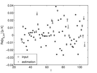
Figure 2: estimated $\mathrm{Re}[a_{E,lm}]$ (m=29)

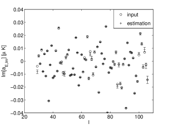
Figure 3: estimated $\mathrm{Im}[a_{E,lm}]$ (m=29)

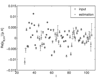
Figure 4: estimated $\mathrm{Re}[a_{B,lm}]$ (m=29)

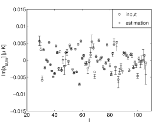
Figure 5: estimated $\mathrm{Im}[a_{B,lm}]$ (m=29)

8 DISCUSSION

Visibilities associated with the CMB polarization can be expressed as a linear sum of spherical harmonic coefficients $a_{\pm 2,lm}$ of the CMB polarization. The linear weight for $a_{\pm 2,lm}$ depends on the observational configuration, and spherical harmonic number $l,m$. Since an interferometer is sensitive over a finite range of multipoles. The spherical harmonic coefficients ($l_{0}\leq l\leq l_{1}$) can be determined by fitting $a_{\pm 2,lm}$ for visibilities of various observational configuration. Once $a_{\pm 2,lm}$ are determined, $a_{E,lm}$ and $a_{B,lm}$ are easily obtained via Eq. 5 and 5. The linear weights $b_{\pm 2,lm}$, which map visibilities to spherical harmonic space, can be computed fast with the aid of the methods discussed in Appendix B. The best-fit value of $a_{2,lm}$ for given visibilities can be found via Eq. 28. It is $\mathcal{O}(\mathsf{m}^{3})$ process, where $\mathsf{m}$ is the number of $a_{2,lm}$ to be determined. Scaling the time taken for the simulated observation says this formalism is computationally feasible for interferometric observation up to multipoles as high as $l\sim 1500$.

Since the formalism introduced in this paper is developed for a satelite-based interferometric observations of all-sky polarization such as the EPIC (Timbie et al., 2006), the antenna pointings in the simulated observation are made over full-sky. Even when antenna pointings are made within a fraction of sky, the matrix $\mathbf{b}$ in Eq. 27 does not become singular, as far as the fraction of sky is big enough in relative to the angular scales the interferometer is sensitive to.

$a_{\pm 2,lm}$ determined by Eq. 28 contain foreground contamination like pixellized maps. With different frequency spectral behavior of foregrounds from the CMB, the foreground contribution can be separated with the multi-frequency data from the CMB down to residual level, which is limited by frequency spectral incoherence and knowledge of polarized foregrounds (Tegmark and Efstathiou, 1996; Tegmark et al., 2000).

There are several sources for E/B mode mixing. Aliasing due to finite pixel size leads to E/B mode mixing at high multipoles and limited sky coverage does at low multipoles. Interferometer observations enable targeting a specific range of multipoles. E/B mode mixing at low multipoles due to limited sky coverage can be made insignificant by designing interferometers to be insensitive to anisotropy at low multipoles. Since the formalism reconstructs $a_{E,lm}$ and $a_{B,lm}$ directly from spherical harmonic space, E/B mixing due to pixellization and ambiguity of E/B mode over the mosaic are insignificant.

We choose the multipole range $l_{0}$ and $l_{1}$ to be the first multipoles, where the window function drops below 1% of its peak value. There are residual contribution from $a_{\pm 2,lm}$ ($l<l_{0}$, $l>l_{1}$). These residuals are another source of estimation error in addition to instrument noise. We can modify noise covariance matrix of Eq. 28 to include $\sum_{l}C_{l}\mathbf{W}_{l,ij}$, where $C_{l}$ and $\mathbf{W}_{l,ij}$ is power spectra and window functions at out-of-bound multipoles. It improves the estimation error due to residuals by giving more weights to the visibilities of less contribution from residuals. But it increases computational load, by making a total noise covariance matrix non-diagonal, while an instrument noise covariance matrix is diagonal to a good approximation (M.P.Hobson and Maisinger, 2002).

We have presented a formalism to reconstruct spherical harmonics of the CMB polarization directly from interferometer observations. The formalism takes advantage of the fact that an interferometer directly probes the Fourier components of sky pattern, and the relation between a Fourier component and spin $\pm 2$ spherical harmonics.

9 ACKNOWLEDGMENTS

The author thanks Gregory Tucker, Peter Timbie, Emory Bunn, Andrei Korotkov and Carolina Calderon for useful discussions. He thanks Douglas Scott for the hospitality during the visit to UBC. He thanks anonymous referees for thorough reading and helpful comments, which led to significant improvements in the paper.

Appendix A CMB polarization basis vectors and antenna coordinate

In all-sky analysis, the CMB polarization at the angular coordinate ($\theta,\phi$) are measured in the local reference frame whose axises are ($\mathbf{\hat{e}}_{\theta}$, $\mathbf{\hat{e}}_{\phi}$, $\mathbf{\hat{e}}_{r}$). Let’s call this coordinate frame ‘the local CMBP frame’ from now on. Consider the polarization observation of antenna pointing ($\theta_{A}$,$\phi_{A}$). A global coordinate frame coincides with the antenna coordinate by Euler rotations $\textbf{R}_{y}(\theta_{A})\,\textbf{R}_{z}(\phi_{A})$. Since a global coordinate frame coincides with the local CMBP frame by Euler rotations $\textbf{R}_{y}(\theta)\,\textbf{R}_{z}(\phi)$, the Euler Rotations $\textbf{R}_{z}(\gamma)\,\textbf{R}_{y}(\beta)\,\textbf{R}_{z}(\alpha)$ coincides the antenna coordinate frame with the local CMBP frame, where $\textbf{R}_{z}(\gamma)\,\textbf{R}_{y}(\beta)\,\textbf{R}_{z}(\alpha)\,\textbf{R}_{y}(\theta_{A})\,\textbf{R}_{z}(\phi_{A})=\textbf{R}_{y}(\theta)\,\textbf{R}_{z}(\phi)$. Therefore, the local CMBP frame is in rotation from the antenna coordinate by the Euler angles $(\alpha,\beta,\gamma)$ as follows:

$$\alpha = \tan^{-1}\left[\frac{\sin\theta\sin(\phi-\phi_{A})}{\sin\theta\cos\theta_{A}\cos(\phi-\phi_{A})-\cos\theta\sin\theta_{A}}\right],$$

$$\beta = \cos^{-1}\left[\cos\theta\cos\theta_{A}+\sin\theta\sin\theta_{A}\cos(\phi-\phi_{A})\right],$$

$$\gamma = \tan^{-1}\left[\frac{\sin\theta_{A}\sin(\phi-\phi_{A})}{-\sin\theta\cos\theta_{A}+\cos\theta\sin\theta_{A}\cos(\phi-\phi_{A})}\right],$$

where the Euler angles $(\alpha,\beta,\gamma)$ can be obtained from $\textbf{R}_{z}(\gamma)\,\textbf{R}_{y}(\beta)\,\textbf{R}_{z}(\alpha)=\textbf{R}_{y}(\theta)\,\textbf{R}_{z}(\phi)\,\textbf{R}^{-1}_{z}(\phi_{A})\,\textbf{R}^{-1}_{y}(\theta_{A})$. In most CMB polarization experiments, where polarizers are attached to the other side of feedhorns, incoming rays go through polarizers after feedhorns. After passing through a feedhorn, an incoming off-axis ray becomes an on-axis ray. Then the local CMBP frame of the ray after the feedhorn system is simply in azimuthal rotation $\alpha+\gamma$ from the antenna coordinate. Therefore, $\Phi$ in Eq. 3 is

$$\Phi = \tan^{-1}\left[\frac{\sin\theta\sin(\phi-\phi_{A})}{\sin\theta\cos\theta_{A}\cos(\phi-\phi_{A})-\cos\theta\sin\theta_{A}}\right]$$

$$+\tan^{-1}\left[\frac{\sin\theta_{A}\sin(\phi-\phi_{A})}{-\sin\theta\cos\theta_{A}+\cos\theta\sin\theta_{A}\cos(\phi-\phi_{A})}\right].$$

Appendix B Computing linear weights

${b_{\pm 2,lm}}$ needs be computed to determine $a_{2,lm}$ ($l_{0}\leq l\leq l_{1}$) via Eq. 28. It can be computed in the baseline coordinate where a baseline coincides with the $x$ axis of the coordinate. In computing ${b_{\pm 2,lm}}$ in the baseline coordinate, spin $\pm 2$ spherical harmonics, which are defined in the global coordinate, are related to spin $\pm 2$ spherical harmonics in the baseline coordinate with a rotation matrix [Challinor and Lewis, 2005]. Let’s choose Galactic coordinate as the global reference coordinate for the CMB. Consider the polarization observation, whose antenna pointing is in the direction of Galactic coordinate ($\ell$,$b$). The baseline is assumed to be on the aperture plane. Then, the baseline coordinate is the coordinate system rotated from Galactic coordinate by Euler rotation $\mathcal{R}(\ell,\frac{\pi}{2}-b,\phi_{\mathbf{u}})$, where $\phi_{\mathbf{u}}$ is the rotation around the axis of antenna pointing. Computed in the baseline coordinate, $b_{\pm 2,lm}$ are

$$b_{2,lm} = \int d\nu\,f(\nu)\int^{\pi}_{0}\mathrm{d}(\theta^{\prime})\sin\theta^{\prime}A(\theta^{\prime})$$ (35)

$$\times\int^{2\pi}_{0}\mathrm{d}\phi^{\prime}\>\sum_{m^{\prime}}\mathsf{D}^{l}_{m^{\prime}m}(\ell,\frac{\pi}{2}-b,\phi_{\mathbf{u}})\;{}_{2}Y_{lm^{\prime}}(\theta^{\prime},\phi^{\prime})$$

$$\times\mathrm{e}^{\mathrm{i}(2\pi u\sin\theta^{\prime}\cos\phi^{\prime}-2(\psi-\phi_{\mathbf{u}})+2\phi^{\prime})}$$

$$= -\mathrm{e}^{-\mathrm{i}2\psi}\sqrt{\pi(2l+1)}$$

$$\times\sum_{m^{\prime}}\mathrm{e}^{\mathrm{i}(m^{\prime}\frac{\pi}{2}+2\phi_{\mathbf{u}})}\;\mathsf{D}^{l}_{m^{\prime}m}(\ell,\frac{\pi}{2}-b,\phi_{\mathbf{u}})$$

$$\times\int^{1}_{-1}\mathrm{d}(\cos\theta^{\prime})A(\theta^{\prime})[F_{1,lm^{\prime}}(\theta^{\prime})+F_{2,lm^{\prime}}(\theta^{\prime})]$$

$$\times\int d\nu\,f(\nu)J_{m^{\prime}+2}(2\pi\sin\theta^{\prime}u),$$

$$b_{-2,lm} = \int d\nu\,f(\nu)\int^{1}_{-1}\mathrm{d}(\cos\theta^{\prime})A(\theta^{\prime})$$ (36)

$$\times\int^{2\pi}_{0}\mathrm{d}\phi^{\prime}\>\sum_{m^{\prime}}\mathsf{D}^{l}_{m^{\prime}m}(\ell,\frac{\pi}{2}-b,\phi_{\mathbf{u}})\;{}_{-2}Y_{lm^{\prime}}(\theta^{\prime},\phi^{\prime})$$

$$\times\mathrm{e}^{\mathrm{i}(2\pi u\sin\theta^{\prime}\cos\phi^{\prime}+2(\psi-\phi_{\mathbf{u}})-2\phi^{\prime})}$$

$$= -\mathrm{e}^{\mathrm{i}2\psi}\sqrt{\pi(2l+1)}$$

$$\times\sum_{m^{\prime}}\mathrm{e}^{\mathrm{i}(m^{\prime}\frac{\pi}{2}-2\phi_{\mathbf{u}})}\;\mathsf{D}^{l}_{m^{\prime}m}(\ell,\frac{\pi}{2}-b,\phi_{\mathbf{u}})$$

$$\times\int^{1}_{-1}\mathrm{d}(\cos\theta^{\prime})A(\theta^{\prime})[F_{1,lm^{\prime}}(\theta^{\prime})-F_{2,lm^{\prime}}(\theta^{\prime})]$$

$$\times\int d\nu\,f(\nu)J_{m^{\prime}-2}(2\pi\sin\theta^{\prime}u),$$

where $J_{n}$ is the $n$th order ordinary Bessel function. It turns out that computing $b_{\pm 2,lm}$ via Eq. 35 and 36 suffers from serious numerical precision problem especially for high multipole ($l>60$), which are due to machine floating-point rounding error occurring in the multiplication with the rotation matrix $\mathsf{D}^{l}_{m^{\prime}m}(\mathcal{R})$. Besides the numerical precision problem, the huge time required for computing the rotation matrix $\mathsf{D}^{l}_{m^{\prime}m}(\mathcal{R})$ makes Eq. 35 and Eq. 36 lose most of merits gained by the availability of analytic integration over azimuthal angle. For these reasons, in the simulated observation of §7 we computed $b_{\pm 2,lm}$ in a fixed CMB frame with Eq. 4 and 4. In Eq. 4 and 4, we have rearranged the order of integration and replaced the integration over continuum with sum over finite elements, which are as follows:

$$b_{2,lm} = \sqrt{\frac{2l+1}{4\pi}}\mathrm{e}^{-\mathrm{i}2\psi}\Delta\theta\Delta\phi\Delta\nu$$

$$\times\sum_{i}\sin\theta_{i}(F_{1,lm}(\theta_{i})+F_{2,lm}(\theta_{i}))$$

$$\times\sum_{j}\mathrm{e}^{\mathrm{i}m\phi_{j}}\mathrm{e}^{\mathrm{i}2\Phi(\hat{\mathbf{n}})}\sum_{k}f(\nu_{k})A(\hat{\mathbf{n}},\hat{\mathbf{n}}_{A})\mathrm{e}^{\mathrm{i}(2\pi\mathbf{u}_{k}\cdot\hat{\mathbf{n}})},$$

$$b_{-2,lm} = \sqrt{\frac{2l+1}{4\pi}}\mathrm{e}^{\mathrm{i}2\psi}\Delta\theta\Delta\phi\Delta\nu$$

$$\times\sum_{i}\sin\theta_{i}(F_{1,lm}(\theta_{i})-F_{2,lm}(\theta_{i}))$$

$$\times\sum_{j}\mathrm{e}^{\mathrm{i}m\phi_{j}}\mathrm{e}^{-\mathrm{i}2\Phi(\hat{\mathbf{n}})}\sum_{k}f(\nu_{k})A(\hat{\mathbf{n}},\hat{\mathbf{n}}_{A})\mathrm{e}^{\mathrm{i}(2\pi\mathbf{u}_{k}\cdot\hat{\mathbf{n}})}.$$

Legendre functions in $F_{1,lm}(\theta)$ and $F_{2,lm}(\theta)$ are computed with the following recurrence relation for $x=\cos\theta$ [Press et al., 1992]:

$$(l-m)P^{m}_{l} = x(2l-1)P^{m}_{l-1}-(l+m-1)P^{m}_{l-2},$$

$$P^{m}_{m} = (-1)^{m}(2m-1)!!(1-x^{2})^{m.2},$$

$$P^{m}_{m+1} = x(2m+1)P^{m}_{m}.$$

When an interferometer is sensitive to multipole range $l_{0}\leq l\leq l_{1}$, $b_{\pm 2,lm}$ of $l$ up to $l_{1}$ should be computed. As shown in Eq. 8, Eq. 9, Eq. 10 and Eq. 11, ${}_{\pm 2}Y_{lm}$ is the product of Legendre functions and $e^{im\phi}$. Legendre functions of multipole $l$ varies on angular scale down to $\theta\approx 180^{\circ}/l$. With Nyquist-Shannon Sampling theorem [Press et al., 1992], the integration over $\theta$ should be done with $\Delta\theta<\frac{180^{\circ}}{2l_{1}}$. Since ‘$e^{im\phi}$’ consisting of ${}_{\pm 2}Y_{lm}$ is periodic over $\phi=360^{\circ}/m$, the integration over $\phi$ should be also done with $\Delta\phi<\frac{360^{\circ}}{2l_{1}}$.

The summation of index $j$ below, which is part of Eq. B and B, is equivalent to discrete Fourier Transform:

$$\sum_{j}\mathrm{e}^{\mathrm{i}m\phi_{j}}\left[\mathrm{e}^{\mathrm{i}2\Phi(\hat{\mathbf{n}})}\sum_{k}f(\nu_{k})A(\hat{\mathbf{n}},\hat{\mathbf{n}}_{A})\mathrm{e}^{\mathrm{i}2\pi\mathbf{u}_{k}\cdot\hat{\mathbf{n}}}\right]$$

. Discrete Fourier Transform, which is the process of $\mathcal{O}(\mathcal{N}^{2})$, can be carried out in $\mathcal{O}(\mathcal{N}\log_{2}\mathcal{N})$ with Fast Fourier Transform [Press et al., 1992, Muciaccia et al., 1997]. Since it is easiest to carry out Fast Fourier Transform on data of number which is a power of two, $\Delta\phi$ was chosen to be $360^{\circ}/(2^{\lceil\log_{2}(2l_{1})\rceil})$, where $\lceil\,\rceil$ denotes the smallest integer larger than or equal to the argument. Choosing the optimal size for $\Delta\theta$ and $\Delta\phi$ and using Fast Fourier Transform enables the numerical computation of $b_{\pm 2,lm}$ feasible in a reasonable amount of time even for interferometers of high $u$. We set the value for the integration cell to be zero and skips computing the rest of terms, when the beam function $A(\hat{\mathbf{n}},\hat{\mathbf{n}}_{A})$ for the integration cell is smaller than $.1\%$ of its peak value. In integration over bandwidth, $\sum_{k}f(\nu_{k})A(\hat{\mathbf{n}},\hat{\mathbf{n}}_{A})e^{i2\pi\mathbf{B}\frac{\nu_{k}}{c}\cdot\hat{\mathbf{n}}}$, an interference term of index $k$ is computed from a term of index $k-1$ as follows so that we can avoid computing time-consuming trigonometric function for each index $k$:

$$\mathrm{e}^{\mathrm{i}2\pi\frac{\nu_{k}}{c}\mathbf{B}\cdot\hat{\mathbf{n}}}=$$

$$(\cos(\frac{2\pi\>\Delta\nu}{c}\mathbf{B}\cdot\hat{\mathbf{n}})+\mathrm{i}\sin(\frac{2\pi\>\Delta\nu}{c}\mathbf{B}\cdot\hat{\mathbf{n}}))\mathrm{e}^{\mathrm{i}2\pi\frac{\nu_{k-1}}{c}\mathbf{B}\cdot\hat{\mathbf{n}}},$$

where the computed value of $\cos(\frac{2\pi\>\Delta\nu}{c}\mathbf{B}\cdot\hat{\mathbf{n}})$ and $\sin(\frac{2\pi\>\Delta\nu}{c}\mathbf{B}\cdot\hat{\mathbf{n}})$ are repeatedly used.

Appendix C Estimation in the absence of noise

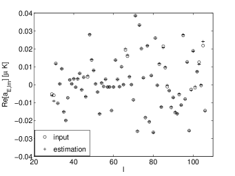
Figure 6: estimated $\mathrm{Re}[a_{E,lm}]$ (m=29) in absence of noise

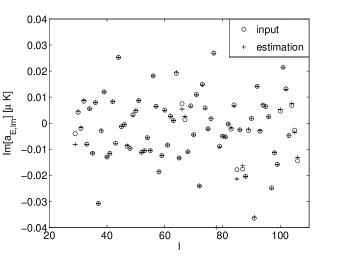
Figure 7: estimated $\mathrm{Im}[a_{E,lm}]$ (m=29) in absence of noise

Estimated $a_{2,lm}$ ($29\leq l\leq 106,\;\;m=29,\,0,\,-29)$ in absence of noise are shown together with the input $a_{2,lm}$ value in Fig. 6, 7, 8, and 9. We assumed the same configuration with the simulated observation in §7 except for the absence of noise. Small discrepancies between estimation and the input values, in spite of no noise, are attributed to residual error. As mentioned in §7, the residual error results from the contribution of $a_{2,lm}$ in the multipoles outside the cutoff region, since we determined $a_{2,lm}$ only over the multipoles where the window function is greater than 1% of its peak value. Some features of methods to facilitate $b_{2,lm}$ computation, which are discussed in Appendix B, sacrifice the numerical precision, which also contributes to the discrepancies.

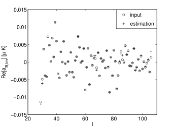
Figure 8: estimated $\mathrm{Re}[a_{B,lm}]$ (m=29) in absence of noise

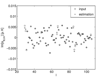
Figure 9: estimated $\mathrm{Im}[a_{B,lm}]$ (m=29) in absence of noise

References

- Arfken and Weber [2000] George B. Arfken and Hans J. Weber. Mathematical Methods for Physicists. Academic Press, San Diego, CA USA, 5th edition, 2000.
- Barkats et al. [2005] D. Barkats, C. Bischoff, P. Farese, L. Fitzpatrick, T. Gaier, J. O. Gundersen, M. M. Hedman, L. Hyatt, J. J. McMahon, D. Samtleben, S. T. Staggs, K. Vanderlinde, and B. Winstein. First measurements of the polarization of the cosmic microwave background radiation at small angular scales from capmap. Astrophys. J. Lett., 619:127, 2005.
- Challinor and Lewis [2005] Anthony Challinor and Antony Lewis. Lensed CMB power spectra from all-sky correlation functions. Phys. Rev. D, 71, 2005.
- Dodelson [2003] Scott Dodelson. Modern Cosmology. Academic Press, 2nd edition, 2003.
- Efstathiou [2006] G. Efstathiou. Hybrid estimation of CMB polarization power spectra. Mon. Not. R. Astron. Soc., 370:343, 2006.
- Gorski et al. [2005] K. M. Gorski, E. Hivon, A. J. Banday, B. D. Wandelt, F. K. Hansen, M. Reinecke, and M. Bartelman. HEALPix – a framework for high resolution discretization, and fast analysis of data distributed on the sphere. Astrophys. J., 622:759, 2005.
- Hinshaw and et al. [2007] G. Hinshaw and et al. Three-year Wilkinson Microwave Anisotropy Probe (WMAP) observations: Temperature analysis. Astrophys.J.Suppl., 170:288, 2007. http://lambda.gsfc.nasa.gov.
- Kamionkowski et al. [1997] Marc Kamionkowski, Arthur Kosowsky, and Albert Stebbins. Statistics of cosmic microwave background polarization. Phys. Rev. D, 55:7368, 1997.
- Korotkov et al. [2006] Andrei L. Korotkov, Jaiseung Kim, Gregory S. Tucker, Amanda Gault, Peter Hyland, Siddharth Malu, Peter T. Timbie, Emory F. Bunn, Evan Bierman, Brian Keating, Anthony Murphy, Créidhe O’Sullivan, Peter A. Ade, Carolina Calderon, and Lucio Piccirillo. The millimeter-wave bolometric interferometer. In Jonas Zmuidzinas, Wayne S. Holland, Stafford Withington, and William D. Duncan, editors, Millimeter and Submillimeter Detectors and Instrumentation for Astronomy III: Proceedings of the SPIE, volume 6275, Bellingham, WA USA, Jun 2006. SPIE, The International Society for Optical Engineering.
- Kovac et al. [2002] J. Kovac, E. M. Leitch, C. Pryke, J. E. Carlstrom, N. W. Halverson, and W. L. Holzapfel. Detection of polarization in the cosmic microwave background using DASI. Nature, 420:772, 2002.
- Kraus [1986] J. Kraus. Radio Astronomy. Cygnus-Quasar Books, Powell, Ohio USA, 2nd edition, 1986.
- Lawson [2006] P. Lawson, editor. Principles of Long Baseline Stellar Interferometry. Wiley-Interscience, Mississauga, Ontario Canada, 2006.
- Leitch et al. [2002] E. M. Leitch, J. M. Kovac, C. Pryke, B. Reddall, E. S. Sandberg, M. Dragovan, J. E. Carlstrom, N. W. Halverson, and W. L. Holzapfel. Measurement of polarization with the degree angular scale interferometer. Nature, 420:763, 2002.
- Leitch et al. [2005] Erik M. Leitch, J. M. Kovac, N. W. Halverson, J. E. Carlstrom, C. Pryke, and M. W. E. Smith. DASI three-year cosmic microwave background polarization results. Astrophys. J., 624:10–20, 2005.
- Lewis et al. [2000] Antony Lewis, Anthony Challinor, and Anthony Lasenby. Efficient computation of CMB anisotropies in closed FRW models. Astrophys. J., 538:473, 2000. http://camb.info/.
- Montroy et al. [2006] T. E. Montroy, P. A. R. Ade, J. J. Bock, J. R. Bond, J. Borrill, A. Boscaleri, P. Cabella, C. R. Contaldi, B. P. Crill, P. de Bernardis, G. De Gasperis, A. de Oliveira-Costa, G. De Troia, G. di Stefano, E. Hivon, A. H. Jaffe, T. S. Kisner, W. C. Jones, A. E. Lange, S. Masi, P. D. Mauskopf, C. J. MacTavish, A. Melchiorri, P. Natoli, C. B. Netterfield, E. Pascale, F. Piacentini, D. Pogosyan, G. Polenta, S. Prunet, S. Ricciardi, G. Romeo, J. E. Ruhl, P. Santini, M. Tegmark, M. Veneziani, and N. Vittorio. A measurement of the CMB ¡ee〉 spectrum from the 2003 flight of BOOMERANG. Astrophys. J., 647:813, 2006.
- M.P.Hobson and Maisinger [2002] M.P.Hobson and Klaus Maisinger. Maximum-likelihood estimation of the CMB power spectrum from interferometer observations. Mon. Not. R. Astron. Soc., 334:569, 2002.
- Muciaccia et al. [1997] P. F. Muciaccia, P. Natoli, and N. Vittorio. Fast spherical harmonic analysis: A quick algorithm for generating and/or inverting full-sky, high-resolution cosmic microwave background anisotropy maps. Astrophys. J. Lett., 488:123523, 1997.
- Page et al. [2006] L. Page, G. Hinshaw, E. Komatsu, M. R. Nolta, D. N. Spergel, C. L. Bennett, C. Barnes, R. Bean, O. Dore’, M. Halpern, R. S. Hill, N. Jarosik, A. Kogut, M. Limon, S. S. Meyer, N. Odegard, H. V. Peiris, G. S. Tucker, L. Verde, J. L. Weiland, E. Wollack, and E. L. Wright. Three year wilkinson microwave anisotropy probe (WMAP) observations: Polarization analysis. Accepted by ApJ, 2006.
- Park and Ng [2004] Chan-Gyung Park and Kin-Wang Ng. E/B separation in CMB interferometry. Astrophys. J., 609:15, 2004.
- Park et al. [2003] Chan-Gyung Park, Kin-Wang Ng, Changbom Park, Guo-Chin Liu, and Keiichi Umetsu. Observational strategies of CMB temperature and polarization interferometry experiments. Astrophys. J., 589:67, 2003.
- Press et al. [1992] William H. Press, Brian P. Flannery, Saul A. Teukolsky, and William T. Vetterling. Numerical Recipes in C : The Art of Scientific Computing. Cambridge University Press, 2nd edition, 1992.
- Readhead et al. [2004] A. C. S. Readhead, S. T. Myers, T. J. Pearson, J. L. Sievers, B. S. Mason, C. R. Contaldi, J. R. Bond, R. Bustos, P. Altamirano, C. Achermann, L. Bronfman, J. E. Carlstrom, J. K. Cartwright, S. Casassus, C. Dickinson, W. L. Holzapfel, J. M. Kovac, E. M. Leitch, J. May, S. Padin, D. Pogosyan, M. Pospieszalski, C. Pryke, R. Reeves, M. C. Shepherd, and S. Torres. Polarization observations with the cosmic background imager. Science, 306:836, 2004. http://www.astro.caltech.edu/ tjp/CBI/press2/index.html.
- Rohlfs and Wilson [2003] K. Rohlfs and T. L. Wilson. Tools of Radio Astronomy. Springer-Verlag, New York, NY USA, 4th edition, 2003.
- Tauber [2000] J. A. Tauber. The Planck mission: Overview and current status. Astrophysical Letters and Communications, 37:145, 2000. http://planck.esa.int.
- Tegmark and Efstathiou [1996] M. Tegmark and G. Efstathiou. A method for subtracting foregrounds from multi-frequency CMB sky maps. Mon. Not. R. Astron. Soc., 281:1297, 1996.
- Tegmark et al. [2000] Max Tegmark, Daniel J. Eisenstein, Wayne Hu, and Angelica de Oliveira-Costa. Foregrounds and forecasts for the cosmic microwave background. Astrophys. J., 530:133, 2000.
- Thompson et al. [2001] A. Richard Thompson, James M. Moran, and George W. Swenson, Jr. Interferometry and synthesis in radio astronomy. Wiley-Intescience Publication, Mississauga, Ontario Canada, 2nd edition, 2001.
- Timbie et al. [2006] P. T. Timbie, G. S. Tucker, P. A. R. Ade, S. Ali, E. Bierman, E. F. Bunn, C. Calderon, A. C. Gault, P. O. Hyland, B. G. Keating, J. Kim, A. Korotkov, S. Malu, P. Mauskopf, J. A. Murphy, C. O’Sullivan, L. Piccirillo, and B. D. Wandelt. The einstein polarization interferometer for cosmology (EPIC) and the millimeterwave bolometric interferometer (MBI). New Astronomy Reviews, 50:999–1008, 2006.
- Tucker et al. [2003] G. S. Tucker, J. Kim, P. Timbie, S. Alib, L. Piccirilloc, and C. Calderon. Bolometric interferometry: the millimeter-wave bolometric interferometer. New Astronomy Reviews, 47:1173–1176, 2003.
- Zaldarriaga [1998a] M. Zaldarriaga. CMB polarization experiments. Astrophys. J., 503:1, 1998a.
- Zaldarriaga and Seljak [1997] M. Zaldarriaga and U. Seljak. An all-sky analysis of polarization in the microwave background. Phys. Rev. D, 55:1830, 1997.
- Zaldarriaga [1998b] Matias Zaldarriaga. Fluctuations in the Cosmic Microwave Background. PhD thesis, MIT, 1998b.