Inferring the Magnetic Fields of Magnetars from their X-ray Spectra

Abstract

We present the first self-consistent theoretical models of magnetar spectra that take into account the combined effects of the stellar atmosphere and its magnetosphere. We find that the proton cyclotron lines that are already weakened by atmospheric effects become indistinguishable from the continuum for moderate scattering optical depths in the magnetosphere. Furthermore, the hard excess becomes more pronounced due to resonant scattering and the resulting spectra closely resemble the observed magnetar spectra. We argue that while the absence of proton cyclotron lines in the observed spectra are inconclusive about the surface field strengths of magnetars, the continuum carries nearly unique signatures of the field strength and can thus be used to infer this quantity. We fit our theoretical spectra with a phenomenological two-blackbody model and compare our findings to source spectra with existing two-blackbody fits. The field strengths that we infer spectroscopically are in remarkable agreement with the values inferred from the period derivative of the sources assuming a dipole spindown. These detailed predictions of line energies and equivalent widths may provide an optimal opportunity for measuring directly the surface field strengths of magnetars with future X-ray telescopes such as Constellation-X.

1 Introduction

Anomalous X-ray Pulsars (AXPs) and Soft Gamma-ray Repeaters (SGRs) are two similar classes of neutron stars thought to be powered by ultrastrong magnetic fields (Duncan & Thompson, 2002). Initially identified by their pulsed soft X-ray (Fahlman & Gregory, 1981) and $\gamma$-ray emissions (Mazets & Golenetskii, 1981), respectively, they are by now observed in multiple wavebands, exhibiting a variety of interesting and complex phenomena (see, e.g., Woods & Thompson, 2004; Wang et al., 2006; Camilo et al., 2006). However, their persistent thermal-like X-ray spectra (with kT $\sim$ 0.3-0.6 keV) and their X-ray luminosities ($L_{X}\sim 10^{34-36}$ ergs/s) that significantly exceed their spin-down luminosities remain as a defining characteristic (e.g., Mereghetti & Stella 1995) and has been the subject of numerous studies.

Empirical models of the observed X-ray spectra of AXP & SGRs have typically required, in addition to a blackbody component, a power-law component, with photon indices ranging between 2.0 and 4.5, or a second blackbody (see, e.g., Woods & Thompson 2004). Although such modelling is adequate for descriptive purposes, more detailed and physically motivated calculations have recently been performed, focusing on the effects of either neutron star atmospheres or their magnetospheres on the X-ray spectra.

Radiative equilibrium models of highly magnetized neutron star atmospheres have been developed recently by numerous authors focusing on different physical processes. Full angle- and polarization-dependent scattering has been incorporated by Özel (2001) and Lloyd (2003). The effects of vacuum polarization resonance were treated completely, including the resonant coupling of modes, by Özel (2001) and Lloyd (2003), and approximately by Ho & Lai (2003) through a probabilistic mode conversion approach. Ion cyclotron lines were calculated by Zane et al. (2001), Ho & Lai (2001), and Özel (2003). Finally, the effects of the two-dimensional structure of the magnetic field were considered by Lloyd (2003) and partial ionization in the atmosphere by Ho & Lai (2003). Most models predict significant deviations from a Planckian spectrum with hard excess that depends on the magnetic field strength as well as absorption features at the ion cylotron frequency that are somewhat suppressed by the vacuum polarization resonance.

The surface emission from a neutron star is processed by its magnetosphere before it reaches a distant observer. Goldreich & Julian (1969) showed that there is a minimum plasma density given by $n=7\times 10^{-2}\it{B}/\it{P}$ $\rm{cm}^{-3}$ in the magnetosphere of a neutron star (where $\it{B}$ is the magnetic field strength in Gauss and $\it{P}$ is the stellar spin period in seconds). If the magnetospheric plasma density is equal to this minimum Goldreich & Julian density, Mikhailovskii et al. (1982) showed that scattering of the surface emission by such a plasma is not important in the X-ray regime. However, in the case of magnetars, Thompson et al. (2002) showed that large-scale currents flowing in the magnetosphere result in much larger particle densities such that resonant cyclotron scattering can be an effective mechanism to modify the emitted spectrum from the surface of a neutron star. This has been proposed as an alternative to the surface models to explain the power-law tail of X-ray spectra of AXPs and SGRs. Inspired by this idea, Lyutikov & Gavriil (2006) calculated the effects of resonant cyclotron scattering on a photon emitted by a Planckian source in the magnetosphere of a neutron star. They showed that the initial spectrum can be shifted to higher energies, which gives rise to a high-energy tail.

In the magnetar context, the combined signatures of the atmosphere and the magnetosphere on the spectrum have not been studied to date. In this paper we calculate the emitted spectra from the surface of a highly magnetized neutron star by incorporating all the physical processes that take place in its atmosphere as well as the resonant cyclotron scattering in its magnetosphere. We study the effects of scattering, both on the continuum of the spectrum and the proton cyclotron lines. We use our results to argue that the absence of the proton cyclotron line is not a good indicator of the stellar field strength while the shape of the continuum can be used to infer a combination of the effective temperature and the surface magnetic field strength.

2 Models

We follow the methods discussed in (Özel, 2001, 2003) and Lyutikov & Gavriil (2006) to calculate the emission from a neutron star atmosphere in radiative equilibrium and the resonant cyclotron scattering of photons in the magnetosphere, respectively.

The neutron star atmosphere models are calculated for fully-ionized H plasmas, taking into account the effects of vacuum polarization and ion cyclotron lines. Here, we also incorporate the higher harmonics of the ion cyclotron lines, following Güver & Özel (2006). As in the previous papers, we construct radiative equilibrium atmospheres using a modified Lucy-Unsöld algorithm. The surface emission spectrum is completely defined by the effective temperature $T_{\rm{eff}}$ of the atmosphere, the surface magnetic field strength $B$, and the gravitational acceleration $g$ on the stellar surface. Throughout this paper, we set g=1.9$\times 10^{14}$ cm$\,\rm{s}^{-2}$.

We calculate the effect of the resonant scattering on the spectrum using the Green’s function approach described in Lyutikov & Gavriil (2006). We assume that the magnetic field in the magnetosphere is spherically symmetric, following a $1/r^{3}$ dependence. We solve the radiative transfer equation using a Schwarzschild-Schuster two-stream approximation. The emerging spectrum depends on two parameters: the resonant scattering optical depth

$$\tau\equiv\frac{\pi^{2}e^{2}nr}{3mc\omega_{B}}$$ (1)

and $\beta$, the thermal electron velocity in units of the speed of light. Here, $n$ is the plasma density, $r$ is the radius of the cyclotron scattering region for a given photon energy, $\omega_{B}\equiv eB/mc$ is the cyclotron frequency, e and m are the electron charge and mass, respectively.

3 Results

In order to investigate the effects of scattering on the surface emission spectrum, we have computed model spectra for surface temperatures 0.1-0.5 keV, and for magnetic field strengths covering a range from $10^{13}$ to $10^{15}$ G. We have then processed the emission spectrum through the magnetosphere using the resonant cyclotron scattering model, for optical depth values $\tau$ = 1 - 10 and electron velocity values $\beta$ = 0.1 - 0.5.

Figure 1: The spectra emerging from a magnetar with a surface magnetic field strength of $10^{14}$ G, a surface temperature of 0.3 keV, and different scattering optical depths in the magnetosphere. The equivalent width of the proton cyclotron line decreases and the spectrum at high energies hardens with increasing optical depth.

To illustrate the effects of resonant cyclotron scattering on both the continuum spectrum and the proton cyclotron lines, we plot, in Figure 1, the spectrum emerging from a neutron star with 0.3 keV surface temperature, $10^{14}$ G surface magnetic field strength, and increasing scattering optical depth in the magnetosphere. At photon energies above the peak of the spectrum, the non-Planckian tails already present in the surface spectra become harder. This is caused by the energy gain experienced by the photons at each resonant scattering of the electrons. The deep proton cyclotron absorption features present in the surface spectra are smoothed out as a result of the effect of resonant cyclotron scattering, as also pointed out by Lyutikov & Gavriil (2006). This is in addition to the fact that vacuum polarization resonance in the atmosphere already reduces the equivalent widths of the proton cyclotron features Özel (2001). Note that in Figure 1, we have chosen a surface emission spectrum with particularly strong harmonics of the proton cyclotron line to demonstrate the effects discussed here.

In Figure 2 and Table 1, we show quantitatively the reduction of the equivalent width of the fundamental proton cyclotron line caused by magnetospheric scattering. The atmosphere model calculation in Figure 2 is for a neutron star with a surface magnetic field of $10^{14}$ G and a surface temperature of 0.3 keV. Results for different magnetic field strengths and the harmonics of the cyclotron lines are presented in Table 1. As can be seen in Figure 2, the equivalent widths depend very weakly on the electron velocity $\beta$, but rapidly decrease with scattering optical depth $\tau$. Even a scattering optical depth of unity is enough to reduce the equivalent width of the lines almost by half. For the model parameters used here, this optical depth corresponds to a particle density of $\sim 3\times 10^{16}$ $\rm{cm}^{-3}$, which is $\sim 10^{4}$ times larger than the Goldreich-Julian density for a $10^{14}$ G magnetar with a period of 6s.

Figure 2: The change in the equivalent width of the fundamental proton cyclotron line as a function of optical depth $\tau$, for different values of the electron velocity $\beta$. + sign denotes the equivalent width of the line when no scattering taken into account. The atmospheric calculation is for a magnetic field strength of $4\times 10^{14}$ Gauss and a surface temperature of 0.3 keV.

Table 1: Cyclotron line equivalent widths

Magnetic Field	Line Energy	Equivalent Width (eV)
($10^{14}$ G)	(keV)	$\tau=1$	$\tau=3$	$\tau=5$
0.1	0.063	0.87	0.44	-
0.1	0.126	0.80	0.41	-
1	0.635	27.96	14.61	6.7
1	1.263	19.78	9.54	3.9
4	2.529	35.05	12.02	-
4	5.051	130.29	44.07	14.6
8	5.050	129.68	27.56	-
10	6.295	122.77	-	-

Both vacuum polarization and resonant cyclotron scattering in the magnetosphere have similar effects on the X-ray spectrum of a magnetar. These effects give rise to both reduced widths of cyclotron lines and to non-planckian shapes in the high energy part of the spectrum ($\sim$2.0-10.0 keV). Usually this component is modeled phenomenologically by adding a second blackbody or a power law to a thermal model. In Table 2, we show the results of fitting our calculated spectra with a phenomenological two-blackbody model. Typically, the temperature of the soft blackbody corresponds to the surface temperature of the neutron star, whereas the second blackbody is used to fit the high-energy tail of the spectrum.

Table 2: Phenomenological two-blackbody description of magnetar models

Magnetic Field	Surface Temp.	$\tau=1$		$\tau=3$		$\tau=5$
($10^{14}$ G)	(keV)	$kT_{1}$	$kT_{2}$	$kT_{1}$	$kT_{2}$	$kT_{1}$	$kT_{2}$
1	0.1	0.11	0.36	0.12	0.42	0.13	0.60
2	0.1	0.08	0.14	0.10	0.19	0.10	0.20
4	0.1	0.09	0.18	0.09	0.21	0.10	0.23
6	0.1	0.09	0.20	0.10	0.22	0.10	0.25
8	0.1	0.09	0.20	0.10	0.23	0.10	0.25
10	0.1	0.09	0.20	0.09	0.22	0.10	0.24
1	0.2	0.17	0.51	0.18	0.61	0.19	0.69
2	0.2	0.22	0.66	0.23	0.73	0.25	1.07
4	0.2	0.11	0.27	0.14	0.32	0.16	0.35
6	0.2	0.15	0.32	0.17	0.37	0.19	0.41
8	0.2	0.17	0.35	0.18	0.40	0.19	0.44
10	0.2	0.17	0.36	0.18	0.41	0.19	0.45
1	0.3	0.22	0.62	0.24	0.75	0.26	0.83
2	0.3	0.31	0.83	0.32	0.90	0.32	0.99
4	0.3	0.35	–	0.38	–	0.43	–
6	0.3	0.16	0.38	0.21	0.44	0.24	0.49
8	0.3	0.19	0.41	0.23	0.48	0.25	0.53
10	0.3	0.22	0.44	0.24	0.51	0.26	0.56
1	0.4	0.25	0.70	0.25	0.80	0.27	0.88
2	0.4	0.33	0.86	0.35	0.92	0.38	0.99
4	0.4	0.49	–	0.51	–	0.54	–
6	0.4	0.46	–	0.51	–	0.55	–
8	0.4	0.46	–	0.27	0.57	0.31	0.61
10	0.4	0.20	0.48	0.28	0.57	0.31	0.63
1	0.5	0.26	0.75	0.31	0.87	0.34	0.96
2	0.5	0.44	1.01	0.44	1.07	0.51	1.23
4	0.5	0.60	1.32	0.60	1.47	0.63	1.60
6	0.5	0.53	–	0.58	–	0.63	–
8	0.5	0.54	–	0.59	–	0.65	–
10	0.5	0.56	–	0.30	0.63	0.35	0.70

4 Discussion

The X-ray spectra of magnetars carry signatures of their magnetic field strengths, which determine both the shape of their continuum and the energies and equivalent widths of cyclotron lines. While the detection of cyclotron lines in AXPs and SGRs would yield the most direct measurement of their surface magnetic field strengths, numerous recent searches with Chandra and XMM-Newton have typically resulted only in upper limits that are given in Table 3. The only exception has been the absorption line feature reported for SGR 0526$-$66 by Ibrahim et al. (2003).

Proton cyclotron lines that are more prominent than the current detection limits are predicted by all models of the atmospheric emission from magnetars despite the presence of processes within the stellar atmospheres that reduce their strengths (see, e.g., Zane et al. 2001; Ho & Lai 2003; Özel 2003). This has been used to argue that the surface field strengths of these sources are such that the cyclotron lines are outside of the observed energy range and may be different than the field strengths inferred from the dipole spin-down formula (e.g., Tiengo et al. 2005).

The theoretical predictions, however, are different when we consider the effects of the magnetosphere. As we showed in §3, the proton cyclotron lines are smeared and often become indistinguishable from the continuum even for moderate scattering optical depths. This is because the scattering of the surface photons in the resonant layers in the magnetosphere broadens any spectral feature due to the random motions of the resonant electrons. It is, therefore, not surprising that searches for proton cyclotron lines typically yield no detections. This also shows that the absence of cyclotron lines is not a good indicator of the magnetic field strength of the neutron star.

The magnetic field leaves its imprint also on the continuum via both atmospheric and magnetospheric processes. On the one hand, these two processes work in tandem to strengthen the observable continuum signature: Compton upscattering hardens the high energy excess already present because of atmospheric effects. On the other hand, the exact shape and hardness of the resulting spectrum depends also on the strength of the unscattered cyclotron line, especially if it occurs at energies above the peak of the X-ray emission. This is because, even though the line is not visible as a distinct feature, it still causes a suppression of the continuum spectrum. As a result, when we use a phenomenological two-blackbody spectral model to describe the theoretical spectra, the inferred blackbody temperatures depend strongly and not monotonically on the magnetic field strength. We show this effect in Figure 3. Note that we have not applied redshift corrections to the temperatures obtained by fitting two blackbodies to our theoretical spectra. Applying such a correction only shifts the predicted correlations between the temperatures along the diagonal without affecting the qualitative result.

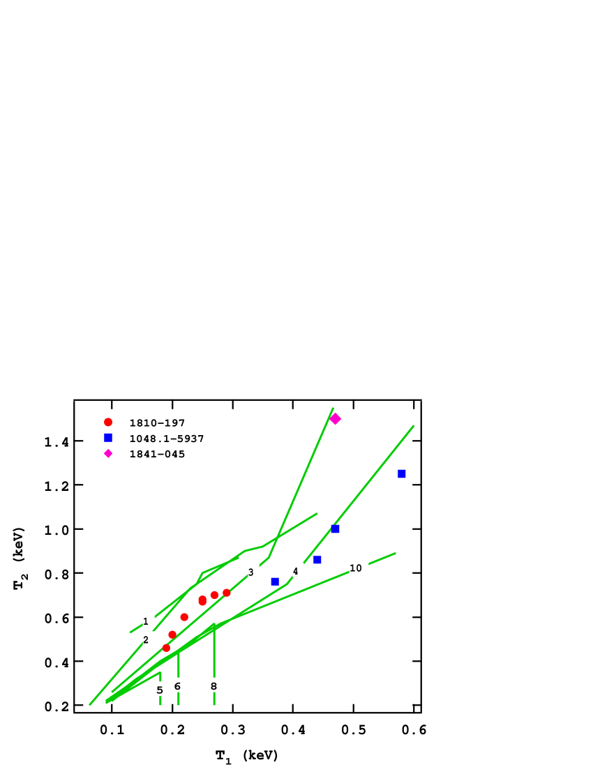
Figure 3: The temperatures of two black bodies used to fit our theoretical spectra for models with different magnetic field strengths in units of $10^{14}$ G (solid lines) as well as the temperatures inferred from multiple observations of three magnetars (filled markers).

The qualitative dependence of the two blackbody temperatures $T_{1}$ and $T_{2}$ changes dramatically at magnetic field strength $\sim 5\times 10^{14}$ G, where the unscattered cyclotron line is the strongest (see Table 1). For all values of the magnetic field strength, the two temperatures in the phenomenological model increase with increasing effective temperature. However, the strength of the second blackbody initially decreases with increasing magnetic field, becoming negligible at moderate effective temperatures for $B\sim 5\times 10^{14}$ G. At even stronger fields, the second blackbody again becomes more prominent.

In Table 2, we show the temperatures of the two blackbodies that represent the observed X-ray spectra of several AXPs and SGRs and compare them in Figure 3 to the theoretical predictions. It is remarkable that the temperatures of the two blackbodies necessary to fit the source spectra lie in the same narrow range predicted by our theoretical models. More importantly, for the two sources for which multiple observations requiring different temperature pairs exist, the data nearly follow constant field lines. This may provide insight into the evolution of the magnetic field following strong bursts.

Fitting directly the actual theoretical models to the observed spectra of magnetars will provide a good handle on their surface magnetic field strengths. However, even the preliminary comparison shown in Figure 3 results in magnetic field strengths that are remarkably close to those inferred from the spin-down formula for these sources: $2.7\times 10^{14}$ G for XTE 1810$-$197 (Gotthelf & Halpern, 2006), $(2.4-5)\times 10^{14}$ G for 1E 1048.1$-$5947 (Kaspi et al., 2001). This implies that very weak (see Table 1) cyclotron lines are likely to be present in the X-ray spectra of these sources. Detection of such lines with future X-ray telescopes such as Constellation-X will confirm these predictions with direct measurement of the surface magnetic fields of magnetars.

Table 3: Observational upper limits on line equivalent widths

Energy Range	Line Width	Equivalent width (eV)
(keV)	(eV)	SGR 1806-20	SGR 1900+14	1E 1048.1-5947	4U 0142+61
1 - 2	0	-	15	10	-
	100	-	50	20	15
	200	-	50	-	-
2 - 4	0	10	20	20	-
	100	20	30	30	-
	200	60	60	-	70
4 - 5	0	20	20	30
	100	30	35	55
	200	40	50	-
	400	-	-	-	200
5 - 6	0	20	50	60	-
	100	30	75	60	-
	200	40	110	-	-
	500	-	-	-	500
6 - 7	0	10	90	90
	100	25	125	150
	200	30	170	-
7- 8	0	10	35	150
	100	30	85	220
	200	30	100	-

Table 4: Inferred temperatures of two-blackbody fits to magnetar spectra

Source Name	$kT_{1}$	$kT_{2}$	Reference
	keV	keV
1E1048.1-5947	0.47	1.00	Tiengo et al. (2005)
	0.44	0.86
	0.37	0.76
	0.58	1.25	Oosterbroek et al. (1998)
1E1841-045	0.47	1.50	Morii et al. (2003)
XTE 1810-197	0.25	0.68	Gotthelf & Halpern (2006)
	0.29	0.71
	0.27	0.70
	0.25	0.67
	0.22	0.60
	0.20	0.52
	0.19	0.46

References

- Camilo et al. (2006) Camilo, F., Ransom, S.M., Halpern, J.P., Reynolds, J., Helfand, D.J., Zimmerman, N., Sarkissian, J. 2006, Nature, 442, 892
- Duncan & Thompson (2002) Duncan, R.C., & Thompson, C. 1992, ApJ, 392, L9
- Fahlman & Gregory (1981) Fahlman, G.G., & Gregory, P.C. 1981, Nature, 293, 202
- Goldreich & Julian (1969) Goldreich, P., & Julian, W.H. 1967, ApJ, 157, 869
- Gotthelf & Halpern (2006) Gotthelf, E.V., & Halpern, J.P. 2006 (/astro-ph/0608473)
- Güver & Özel (2006) Güver, T., Özel, F. 2006, in preparation
- Ho & Lai (2001) Ho, W.C.G., & Lai, D. 2001, MNRAS, 327, 1081
- Ho & Lai (2003) Ho, W.C.G., & Lai, D. 2003, MNRAS, 338, 233
- Ibrahim et al. (2003) Ibrahim, A.I., Swank, J.H., & Parke, W. 2003, ApJ, 584, L17
- Juett et al. (2002) Juett, A.M., Marshall, H.L., Chakrabarty, D., Schulz, N.S. 2002 ApJ568, L31
- Kaspi et al. (2001) Kaspi, V. M., Gavriil, F. P., Chakrabarty, D., Lackey, J. R., & Muno, M. P. 2001, ApJ, 558, 253
- Lloyd (2003) Lloyd, A.D. 2003, preprint(astro-ph/0303561)
- Lyutikov & Gavriil (2006) Lyutikov, M., & Gavriil, F.P. 2006, MNRAS, 368, 690L
- Mazets & Golenetskii (1981) Mazets, E.P. & Golenetskii, S.V. 1981, ApS&S, 75, 47
- Mereghetti & Stella (1995) Mereghetti, S., & Stella, L. 1995, ApJ, 442, L17
- Mereghetti et al. (2006) Mereghetti, S., Esposito, P., A., Tiengo 2006, (/astro-ph/0608364)
- Mikhailovskii et al. (1982) Mikhailovskii, A.B., Onishcenko, O.G., Suramlishvili, G.I., Sharapov, S.E. 1982, SvA, 8, L369
- Morii et al. (2003) Morii, M., Sato, R., Kataoka, J., Kawai, N. 2003, PASJ, 55, 45
- Oosterbroek et al. (1998) Oosterbroek, T., Parmar, A.N., Mereghetti, S., Israel, G.L. 1998, A&A, 334, 925
- Özel (2001) Özel F., 2001, ApJ, 563, 276
- Özel (2003) Özel F., 2003, ApJ, 583, 402
- Thompson et al. (2002) Thompson C., Lyutikov M., Kulkarni S.R., 2002, ApJ, 574, 332
- Tiengo et al. (2005) Tiengo, A., Mereghetti, S., Turolla, R., Zane, S., Rea, N., Stella, L., Israel, G.L. 2005, A&A, 437, 997
- Tiengo et al. (2006) Tiengo, A., et al. 2006, (/astro-ph/0609319)
- Wang et al. (2006) Wang, Z., Chakrabarty, D., Kaplan, D.L. 2006, Nature, 440, 772
- Woods & Thompson (2004) Woods P.M., Thompson C., 2004, preprint(astro-ph/0406133)
- Zane et al. (2001) Zane, S., Turolla, R., Stella, L., & Treves, A. 2001, ApJ, 560, 384