The Transit Light Curve (TLC) Project.
III. Tres Transits of TrES-1

Abstract

We present $z$ band photometry of three consecutive transits of the exoplanet TrES-1, with an accuracy of 0.15% and a cadence of 40 seconds. We improve upon estimates of the system parameters, finding in particular that the planetary radius is $1.081\pm 0.029$ $R_{\rm Jup}$ and the stellar radius is $0.811\pm 0.020$ $R_{\odot}$. The uncertainties include both the statistical error and the systematic error arising from the uncertainty in the stellar mass. The transit times are determined to within about 15 seconds, and allow us to refine the estimate of the mean orbital period: $P=3.0300737\pm 0.0000026$ days. We find no evidence for star spots or other irregularities that have been previously reported.

1 Introduction

The passage of a planet in front of its parent star is an occasion for celebration and for intensive observations. Transits provide a wealth of information about an exoplanetary system, even when there is little hope of ever resolving the system with adaptive optics, coronagraphy, or interferometry (see, e.g., the recent review by Charbonneau et al. 2006). The dimming events can be recorded photometrically (as first done by Charbonneau et al. 2000 and Henry et al. 2000) and used to determine the planetary and stellar radii. Short-term anomalies in the timing of the transits may betray the presence of moons or other planets (Holman & Murray 2005, Agol et al. 2005), and long-term variations in the light-curve shape should result from orbital precession (Miralda-Escudé 2002), although neither effect has yet been observed. A few stellar absorption lines have been observed to deepen due to absorption by the planetary atmosphere (Charbonneau et al. 2002, Vidal-Madjar et al. 2003). There are also anomalous Doppler shifts due to the Rossiter-McLaughlin effect, which reveal the angle on the sky between the stellar rotation axis and the orbital axis (Queloz et al. 2000; Winn et al. 2005,2006; Wolf et al. 2006). Secondary eclipses—the counterpoints to transits, when the planet passes behind the star—have not yet been detected at optical wavelengths, where the signal would reveal the planetary albedo. However, they have been detected at mid-infrared wavelengths (Charbonneau et al. 2005; Deming et al. 2005, 2006) and are beginning to reveal details of exoplanetary thermal emission.

The aim of the Transit Light Curve (TLC) project is to build a library of high-precision transit photometry. Our main scientific goals are to support all of the transit investigations mentioned above, by refining estimates of the basic system parameters; and to search for secular and short-term variations in transit times and light-curve shapes that would be produced by as-yet undiscovered planets or moons. We have previously reported on TLC observations of the transiting exoplanets XO-1b (Holman et al. 2006) and OGLE-TR-111b (Winn et al. 2006).

In this paper, we present TLC results for TrES-1b, whose discovery by Alonso et al. (2004) was notable for being the first success among the many ground-based, wide-field surveys for transiting planets with bright parent stars. The TrES-1 parent star is 12th magnitude with spectral type K0 V. The planet is a “hot Jupiter” with a mass and radius of approximately 0.8 $M_{\rm Jup}$ and 1.0 $R_{\rm Jup}$, and an orbital period that is almost exactly 3 days. Calculations by Laughlin et al. (2005) have shown that the measured planetary radius is in accordance with models of irradiated hot Jupiters. Charbonneau et al. (2005) have detected thermal emission from the planet. Steffen & Agol (2005) have searched for transit timing anomalies, with null results.

This paper is organized as follows. We describe the observations in the next section, and the photometric procedure in § 3. In § 4, we describe the techniques we used to estimate the physical and orbital parameters, and in § 5 we provide the results, along with a closer look at the characteristics of the photometric noise. A brief summary is given in § 6.

2 Observations

We observed three transits of TrES-1 (on UT 2006 June 9, 12, and 15), corresponding to epochs $E=234$, 235, and 236 of the ephemeris given by Alonso et al. (2004):

$$T_{c}(E)=2,453,186.8060~{}{\mathrm{[HJD]}}+E\times(3.030065~{}{\mathrm{days}}).$$ (1)

We used KeplerCam on the 1.2m (48 in) telescope at the Fred L. Whipple Observatory (FLWO) on Mt. Hopkins, Arizona. KeplerCam has one 4096² Fairchild 486 back-illuminated CCD, with a $23\farcm 1\times 23\farcm 1$ field of view. For our observations we used $2\times 2$ binning, which gives a scale of $0\farcs 68$ per binned pixel, a readout/setup time of 11 s, and a typical readout noise of 7 e^- per binned pixel. We observed through the SDSS $z$ band filter in order to minimize the effect of color-dependent atmospheric extinction on the relative photometry, and to minimize the effect of limb-darkening on the transit light curve. The effective band pass was limited at the blue end by the filter (which has a transmission of 25% at 825 nm, rising to 97% for wavelengths redward of 900 nm) and at the red end by the quantum efficiency of the CCD (which drops from 90% at 800 nm to 25% at 1000 nm).

On each of the three nights, we observed TrES-1 for approximately 6 hr bracketing the predicted midpoint of the transit. We acquired 30 second exposures in good focus. We also obtained dome flat exposures and zero-second (bias) exposures at the beginning and the end of each night.

On the night of UT June 9, we observed under generally light clouds, through an airmass ranging from 1.01 to 1.35. A period of thicker clouds caused about 45 minutes of data following egress to be unusable. There were also small temperature fluctuations ($\sim$0.1 deg min^-1) that proved to cause systematic errors in the photometry, as described in § 3. In addition, the guider was not functioning as intended, causing the position of TrES-1 on the detector to drift by about 20 pixels over the course of the observations. The full-width at half-maximum (FWHM) of stellar images ranged from 2 to 3 binned pixels (1$\farcs$3 to 2$\farcs$0).

The weather was nearly perfect on the nights of UT June 12th and 15th, with no visible clouds. Automatic guiding was functioning, and the pixel position of TrES-1 varied by no more than 4 pixels over the course of each night. On the 12th, the airmass ranged from 1.01 to 1.18, and the FWHM was nearly constant at approximately 2.4 binned pixels (1$\farcs$6). On the 15th, the airmass ranged from 1.01 to 1.20, and the FWHM ranged from 2.5 to 3.5 binned pixels (1$\farcs$7 to 2$\farcs$3).

3 Data Reduction

We used standard IRAF procedures for the overscan correction, trimming, bias subtraction, and flat-field division. We performed aperture photometry of TrES-1 and 12 nearby stars of comparable brightness. Many different aperture sizes were tried in order to find the one that produced the minimum noise in the out-of-transit data. For the three nights, the optimum aperture radii were 7, 8, and 7 pixels ($4\farcs 7$, $5\farcs 4$, and $4\farcs 7$). We subtracted the underlying contribution from the sky, after estimating its brightness within an annulus centered on each star ranging from 30 to 35 pixels in radius.

For each night’s data, the following steps were followed to produce relative photometry of TrES-1: (1) The light curve of each comparison star was normalized to have unit median. (2) A comparison signal was created by taking the mean of all 12 normalized light curves, after rejecting obvious outliers in the comparison star light curves. (3) The light curve of TrES-1 was divided by the comparison signal. Although the transit was obvious, there was a small residual time gradient in the out-of-transit data, a sign of a residual systematic error. (4) To correct for the time gradient and set the out-of-transit flux to unity, the light curve was divided by a linear function of time. This function was determined as part of the model-fitting procedure and will be described in the next section.

For the data from UT June 9, an intermediate step between steps (3) and (4) was necessary. Those data suffered from an additional systematic error, namely, a few “bumps” in the light curve, with amplitude $\sim$0.2% and time scale $\sim$15 minutes. The deviations between this light curve and the light curves based on data from the subsequent nights proved to be well correlated with both the ambient temperature (especially the temperature measured at the mirror cell), and the measured ellipticity of stellar images. Presumably the temperature fluctuations were affecting the focus, which in turn caused differential leakage of light outside the digital apertures. To correct for this systematic error, we used the data from the other two nights to construct a light-curve model (see § 4), and then found the residuals between the UT June 9 data and the model. A linear function provided a good fit to the correlation between the residuals and ellipticity; we used this relation to correct each data point based on the measured ellipticity. We verified that the resulting light curve had residuals that were uncorrelated with temperature, FWHM, and ellipticity. On the other nights, neither the temperature nor the ellipticity varied as much. The data did not have any noticeable correlations with external variables, and no corrections were applied.

To estimate the relative uncertainties in our photometry, we computed the quadrature sum of the errors due to the Poisson noise of the stars (both TrES-1 and the comparison stars), the Poisson noise of the sky background, the readout noise, and the scintillation noise (as estimated according to the empirical formulas of Young 1967 and Dravins et al. 1998). The dominant term is the 0.1% Poisson noise from TrES-1. For the UT June 9 data, an additional error term was included in the sum, equal to one-half the size of the ellipticity-based correction.

The final photometry is given in Table 1, and is plotted in Fig. 1. The quoted uncertainties have been rescaled by a factor specific to each night, such that $\chi^{2}/N_{\rm DOF}=1$ when fitting each night’s data individually (see § 4). The scale factors by which the calculated errors for each night needed to be increased were 1.17, 1.13, and 1.26. A composite light curve, produced by time-shifting the first and last nights’ data appropriately, is shown in Fig. 2. The lower panel shows a time-binned version of the composite light curve, in which the bin size is 3 minutes.

Figure 1: Relative $z$ band photometry of TrES-1. The best-fitting model is shown as a solid line. The residuals (observed $-$ calculated) and the rescaled $1~{}\sigma$ error bars are also shown. The residuals have zero mean but are offset by a constant flux to appear beneath each light curve, for clarity. From top to bottom, the root-mean-squared (RMS) residuals are 0.16%, 0.14%, and 0.15%.

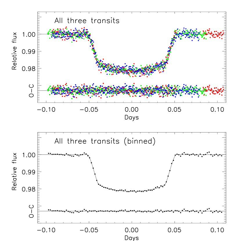
Figure 2: Composite transit light curve of TrES-1. Top. Data from UT June 9, 12, and 15 are shown with red, green, and blue points, respectively. The best-fitting model is shown as a solid line. The residuals (observed $-$ calculated) and the $1~{}\sigma$ error bars are shown beneath each light curve. The mean time between points is 15 seconds, and the RMS residual is 0.15%. Bottom. Same, after binning in time with 3 minute bins. The RMS residual is 0.046%.

4 The Model

To estimate the planetary, stellar, and orbital parameters, we fitted a parameterized model to all of the photometry simultaneously. The model is based on a star and a planet on a circular orbit about the center of mass. The star has a mass $M_{\star}$ and radius $R_{\star}$, and the planet has a mass $M_{p}$ and radius $R_{p}$. The orbit has a period $P$ and an inclination $i$ relative to the sky plane. We define the coordinate system such that $0\arcdeg\leq i\leq 90\arcdeg$. It is often useful to refer to the impact parameter $b\equiv a\cos i/R_{\star}$ (where $a$ is the semimajor axis) rather than the inclination.

We allowed each transit to have an independent value of $T_{c}$, the transit midpoint, rather than forcing them to be separated by exact multiples of the orbital period. This is because we sought to measure or bound any timing anomalies that may indicate the presence of moons or additional planets in the system. Thus, the period $P$ was relevant to the model only through the connection between the total mass and the orbital semimajor axis. We fixed $P=3.030065$ days, the value determined by Alonso et al. (2004). The uncertainty of $0.000008$ days was negligible for this purpose (although we were able to use the resulting values of $T_{c}$ to refine the period estimate, as described in § 5).

The stellar mass cannot be determined from transit photometry alone. Furthermore, the values of $R_{\star}$ and $R_{p}$ that result from fitting the photometry depend on the choice of stellar mass. Our approach was to fix $M_{\star}$ at a value that has been estimated from an analysis of the stellar spectrum (its luminosity class, effective temperature, surface gravity, etc.) and theoretical isochrones, and then use the scaling relations $R_{p}\propto M_{\star}^{1/3}$ and $R_{\star}\propto M_{\star}^{1/3}$ to estimate the systematic error due to the uncertainty in $M_{\star}$. We adopted the value $M_{\star}=0.89\pm 0.05$ $M_{\odot}$ based on the analysis by Sozzetti et al. (2004), noting that this value is also in agreement with independent work by Laughlin et al. (2005) and Santos et al. (2006). The planetary mass $M_{p}$ is nearly irrelevant to the model (except for its minuscule effect on the semimajor axis), but for completeness we use the value $M_{p}=0.76$ $M_{\rm Jup}$ found by Sozzetti et al. (2004).

To calculate the relative flux as a function of the projected separation of the planet and the star, we assumed the limb darkening law to be quadratic,

$$\frac{I_{\mu}}{I_{1}}=1-u_{1}(1-\mu)-u_{2}(1-\mu)^{2},$$ (2)

where $I$ is the intensity, and $\mu$ is the cosine of the angle between the line of sight and the normal to the stellar surface. We employed the analytic formulas of Mandel & Agol (2002) to compute the integral of the intensity over the portion of the stellar disk hidden by the planet. There is a quandary over how to treat the limb darkening parameters when fitting transit photometry. Most previous investigators in this situation have either fixed the parameters at the values calculated with stellar atmosphere models (see, e.g., Jha et al. 2000, Moutou et al. 2004, Laughlin et al. 2005), or allowed them to vary freely (e.g., Brown et al. 2001, Deeg et al. 2001, Winn et al. 2005; see also Knutson et al. 2006, who tried both approaches on the same data). However, the first option is problematic because the stellar atmosphere models are not perfect, and it may be a mistake to trust them so completely. On the other hand, the second option probably allows too much freedom in the limb darkening function, and hence too much uncertainty in the fitted parameter values.

Our approach was to allow $u_{1}$ and $u_{2}$ to be free parameters, but with a mild a priori constraint based on the stellar atmosphere models of Claret (2004). In particular, we added a penalty term to $\chi^{2}$ (see below) to encourage the limb-to-center intensity ratio $I_{0}/I_{1}$ to agree within 20% of the value calculated by Claret (2004) based on the ATLAS quadratic fit ($u_{1}=0.2851$, $u_{2}=0.2849$). We chose the figure of 20% based on a survey of the recent literature in which limb darkening calculations are compared to interferometric and microlensing observations. There seems to be agreement to within 5-20% in the limb-to-center intensity ratio for various stellar types (see, e.g., Abe et al. 2003, Fields et al. 2003, Ohishi et al. 2004, Aufdenberg et al. 2005, Bigot et al. 2006). We also investigated the effect of either tightening or dropping this a priori constraint, as discussed below.

As noted in the previous section, the light curves exhibited a time gradient in the out-of-transit data, probably due to differential extinction between the target star and the comparison stars, or some other systematic error. For this reason, each transit was described with two additional parameters: the out-of-transit flux $f_{\rm oot}$ and a time gradient $\alpha$.

In total, there were 14 adjustable parameters describing 1149 photometric data points. The parameters were $R_{\star}$, $R_{p}$, and $i$; the limb-darkening parameters $u_{1}$ and $u_{2}$; and the values of $T_{c}$, $f_{\rm oot}$ and $\alpha$ for each of the 3 transits. In practice, it was preferable to use the parameters $v_{1}\equiv 2u_{1}+u_{2}$ and $v_{2}\equiv u_{1}-2u_{2}$ rather than $u_{1}$ and $u_{2}$. This is because $v_{1}$ and $v_{2}$ have nearly uncorrelated uncertainties.

We optimized the parameters by using the AMOEBA algorithm (Press et al. 1992, p. 408) to minimize the error statistic

$$\chi^{2}=\sum_{j=1}^{1149}\left[\frac{f_{j}({\mathrm{obs}})-f_{j}({\mathrm{calc}})}{\sigma_{j}}\right]^{2}+\left[\frac{(I_{1}/I_{0})-0.43}{0.086}\right]^{2},$$ (3)

where $f_{j}$(obs) is the flux observed at time $j$, $\sigma_{j}$ is the corresponding uncertainty, and $f_{j}$(calc) is the calculated value. The second term is the a priori constraint on the limb darkening function. As noted in § 3, the uncertainties $\sigma_{j}$ were the calculated uncertainties (based on Poisson noise, scintillation noise, etc.), after multiplication by a factor specific to each night, such that $\chi^{2}/N_{\rm DOF}=1$ when each night’s data was fitted individually. (Our intention was not to test the model, but rather to determine the appropriate weights for the data points.) The optimized model is plotted as a solid line in Figs. 1 and 2. The differences between the observed fluxes and the calculated fluxes are also shown beneath each light curve.

The statistical uncertainties in the fitted parameters were estimated using a Markov Chain Monte Carlo (MCMC) simulation (for a brief introduction, consult appendix A of Tegmark et al. 2004). In this method, a stochastic process is used to create a sequence of points in parameter space that approximates the joint probability distribution of the parameter values, given the data values. The sequence, or “chain,” is generated from an initial point by iterating a “jump function” which can take various forms. Our jump function was the addition of a Gaussian random number to each parameter value. If the new point has a lower $\chi^{2}$ than the previous point, the jump is executed; if not, the jump is only executed with probability $\exp(-\Delta\chi^{2}/2)$. We set the perturbation sizes such that $\sim$25% of jumps are executed. We created 20 independent chains, each with 500,000 points, starting from random initial positions. The first 100,000 points were not used, to minimize the effect of the initial condition. The correlation lengths were $\sim$1000 for the highly covariant parameters $R_{p}$, $R_{\star}$, and $b$, and $\sim$200 for the other parameters. The Gelman & Rubin (1992) $R$ statistic was within 0.2% of unity for each parameter, a sign of good mixing and convergence.

Table 2 gives the results for each parameter, along with some useful quantities derived from the parameters. Among the latter are the times between first and last contact ($t_{\rm IV}-t_{\rm I}$) and between first and second contact ($t_{\rm II}-t_{\rm I}$), which are useful for planning future photometric measurements, and the quantity $(R_{p}/a)^{2}$, which controls the amount of starlight that is reflected from the planet.

Fig. 3 shows the probability distributions for the especially interesting parameters $R_{\star}$, $R_{p}$ and $b$, along with some of the 2-d probability distributions for some correlated parameters. Although the distributions shown in Fig. 3 are somewhat asymmetric about the median, Table 2 reports only the median $p_{\rm med}$ and a single number $\sigma_{p}$ characterizing the statistical error. The value of $\sigma_{p}$ is the average of $|p_{\rm med}-p_{\rm hi}|$ and $|p_{\rm med}-p_{\rm lo}|$, where $p_{\rm lo}$ and $p_{\rm hi}$ are the lower and upper 68% confidence limits. Two-sided formal uncertainties are of little practical significance for $R_{p}$ and $R_{\star}$ because those parameters are subject to a systematic error that is comparable to the statistical error, namely, the covariance with the stellar mass. The size of this systematic error is also given in Table 2. The results for $b$ and $i$ are best regarded as one-sided limits, since central transits are allowed with reasonable probability.

Figure 3: Top row. Probability distributions for the stellar radius $R_{\star}$, planetary radius $R_{p}$, and impact parameter $b\equiv a\cos i/R_{\star}$, based on the MCMC simulations. The arrows mark the values of the parameters that minimize $\chi^{2}$. A solid line marks the median of each distribution, and the dashed lines mark the 68% confidence limits. For $b$, the dashed line marks the 95% confidence upper limit. Middle and bottom rows. Joint probability distributions of those parameters with the strongest correlations. The contours are isoprobability contours enclosing 68% and 95% of the points in the Markov chains. The dotted lines indicate the values of the limb darkening parameters calculated by Claret (2004) using an ATLAS model of a star with $T_{\rm eff}=5250$ K, $\log g=4.5$, [Fe/H] = 0.0, and $\xi_{t}=1.0$ km s^-1.

5 Results

Our results for the planetary and stellar radii are $R_{p}=1.081\pm 0.029$ $R_{\rm Jup}$ and $R_{\star}=0.811\pm 0.020$ $R_{\odot}$. The quoted error in each parameter is the quadrature sum of the statistical error (based on the 68% confidence limits found through the MCMC simulations) and the systematic error (based on the 1 $\sigma$ uncertainty in the stellar mass quoted by Sozzetti et al. 2004). The statistical and systematic errors are comparable in size. The ratio of radii is independent of the stellar mass and is known with greater precision: $R_{p}/R_{\star}=0.13686\pm 0.00082$.

Previous investigators have not had photometry of sufficiently high cadence and signal-to-noise ratio to solve for both $R_{\star}$ and $R_{p}$ simultaneously. Instead, they have used estimates for $R_{\star}$ (as well as $M_{\star}$) based on an analysis of the stellar spectrum and theoretical isochrones. Sozzetti et al. (2004) found $R_{\star}=0.83\pm 0.05$ $R_{\odot}$, and Laughlin et al. (2005) found $R_{\star}=0.83\pm 0.03$ $R_{\odot}$. Our photometry has allowed us to estimate $R_{\star}$ independently, subject only to the fairly weak covariance with $M_{\star}$. Our result of $R_{\star}=0.811\pm 0.020$ $R_{\odot}$ confirms the previous estimates and improves upon their precision.

The planetary radius of $R_{p}=1.081\pm 0.029$ $R_{\rm Jup}$ is also in agreement with (and more precise than) the previous estimates of $1.04^{+0.08}_{-0.05}$ $R_{\rm Jup}$ (Sozzetti et al. 2004) and $1.08\pm 0.05$ $R_{\rm Jup}$ (Laughlin et al. 2005). TrES-1 is an important case study for theoretical models of the structure of hot Jupiters, in part because of the comparison to the intensively studied exoplanet HD 209458. The radius of TrES-1 is smaller by $\sim$20%, despite a similar mass and a similar degree of stellar insolation. Calculations by Laughlin et al. (2005) and Baraffe et al. (2005) have shown that the properties of TrES-1 are generally in line with theoretical expectations, and that HD 209458 is anomalous. This provides the important clue that any mechanism to “inflate” HD 209458 cannot apply to all hot Jupiters of the same mass. Showman & Guillot’s (2002) proposal, that atmospheric circulation patterns deposit a significant fraction of the stellar insolation into the planetary interior, provides no apparent reason why TrES-1 and HD 209458 should be so different, unless perhaps the circulation patterns depend strongly on surface temperature ($\approx$1060 K for TrES-1 and 1130 K for HD 209458). Bodenheimer et al. (2001) proposed that HD 209458 is heated internally by eccentricity tides. Winn & Holman (2005) proposed that HD 209458 is trapped in a Cassini state with nonzero obliquity, causing ongoing heating through obliquity tides. This is naturally a rare occurrence, the implication being that most hot Jupiters (including TrES-1) have a negligible obliquity. Adding to the puzzle, two newly discovered exoplanets also appear to be anomalously large: HAT-P-1 (Bakos et al. 2006) and WASP-1 (Collier Cameron et al. 2006, Charbonneau et al. 2006).

We also confirm that the transit is fairly central, i.e., the trajectory of the planet comes close to the center of the stellar disk. With 95% confidence, $b<0.28$ and $i>88\fdg 4$. All other things being equal, central transits have the maximum possible duration and allow for the greatest number of in-transit measurements (and therefore the greatest signal-to-noise ratio). This makes them favorable for follow-up photometry. However, they are unfavorable for certain applications, such as the measurement of orbital precession through changes in the impact parameter (Miralda-Escudé 2002), or of spin-orbit alignment through the Rossiter-McLaughlin effect (Ohta et al. 2005, Gaudi & Winn 2006). Specifically, a central transit provides little leverage on the determination of the angle $\lambda$ between the projected orbital axis and the projected stellar spin axis, because in that case $\lambda$ is strongly covariant with the stellar rotation rate.

The fitted values of the limb darkening parameters are $u_{1}=0.28\pm 0.06$ and $u_{2}=0.21\pm 0.12$, with a strong covariance as noted previously. In comparison, the values calculated by Claret (2004) are $u_{1}=u_{2}=0.29$. These are in good agreement, which is not surprising because of the a priori constraint on the limb darkening function. If this constraint is dropped, then the optimized limb darkening parameters are $u_{1}=0.36$ and $u_{2}=0.01$ (implying a limb-to-center intensity ratio of 63% instead of the theoretical value of 42%), and the radius estimates become $R_{\star}=0.815$ $R_{\rm Jup}$ and $R_{p}=1.096$ $R_{\rm Jup}$. Thus, by dropping the a priori constraint, the favored values of the radii are driven to larger values, but by less than the $1~{}\sigma$ statistical error determined previously. Conversely, if the limb darkening parameters are held fixed at the Claret (2004) values, the new radius estimates are $R_{\star}=0.810$ $R_{\odot}$ and $R_{p}=1.072$ $R_{\rm Jup}$, again within the $1~{}\sigma$ statistical error of our quoted results. Limb darkening should therefore be considered as another source of systematic error, but one that is no larger than (and is probably smaller than) the systematic error due to the covariance with stellar mass.

The statistical errors in our transit times range from 12 to 17 seconds. We used the ephemeris of Alonso et al. (2004) to compute “observed minus calculated” (O$-$C) residuals for the newly measured transit times, along with 14 of the transit times and the time of secondary eclipse reported by Charbonneau et al. (2005). The residuals are shown in Fig. 4. We fitted a straight line to the transit times as a function of epoch number $E$ to derive a refined ephemeris

$$T_{c}(E)=T_{c}(0)+E\times P,$$ (4)

finding $T_{c}(0)=$ 2,453,186.80603(28) [HJD] and $P=3.0300737(13)$ days, where the numbers in parentheses are the uncertainties in the last 2 digits. It must be noted that a line is not a statistically acceptable fit to the timing data; the value of $\chi^{2}$ is 23.5 with 12 degrees of freedom ($\chi^{2}/N_{\rm dof}=2$). For this reason, we increased all of the errors by a factor of $\sqrt{2}$ before determining the uncertainties in $T_{c}(0)$ and $P$. The poor fit could be a signal that the period is not constant, as assumed, or it could be a signal of systematic errors in the measured times. To be conservative, we recommend basing future predictions on the period $3.0300737$ days but with an uncertainty of $0.0000026$ days, i.e., twice as large as the formal uncertainty. Interestingly, our 3 new measurements are only marginally consistent with a uniform period at the $1~{}\sigma$ level. The transits occur progressively later than expected. Of course, with only 3 measurements this could be a coincidence, but future measurements are motivated by the possible detection of a satellite or additional planet through a periodicity in the residuals.

Figure 4: Transit and secondary-eclipse timing residuals for TrES-1, from Charbonneau et al. (2005) and this work. The calculated times (using the ephemeris of Alonso et al. 2004) have been subtracted from the observed times. The best-fitting line is plotted, representing the updated ephemeris given in Eq. (4) and the text that follows it.

Previous investigators have reported on interesting photometric anomalies in TrES-1 light curves. The review paper by Charbonneau et al. (2006) includes an exquisite light curve obtained with the Hubble Space Telescope in which there is a positive flux excursion relative to the model of $\approx$0.2%, lasting for $\approx$30 minutes (Brown et al., in preparation). The most natural interpretation is that the planet occulted a star spot or group of star spots, a phenomenon anticipated by Silva (2003). We find no evidence for star spots in our data, and can set bounds on spot properties under certain assumptions. For a circular spot much smaller than the planet, the anomaly in the transit light curve caused by the spot occultation is approximately

$$f(R_{\rm spot},I_{\rm spot})=\left(\frac{R_{\rm spot}}{R_{\star}}\right)^{2}\left(1-\frac{I_{\rm spot}}{I_{\star}}\right),$$ (5)

where $R_{\rm spot}$ is the spot radius, $I_{\rm spot}$ is the intensity of the spot, and $I_{\star}$ is the intensity of the unspotted stellar photosphere in the vicinity of the spot. The intensity ratio can be related to the temperature difference via the blackbody formula, as in Eq. (1) of Silva (2003). The duration of sunspot-eclipse totality is $\sim$$2R_{p}/v_{\rm orb}$, or 20 minutes, if the spot lies exactly on the transit chord. A more likely impact parameter of 0.5 would lead to a duration of about 15 minutes. By averaging our data into 15 minute time bins, we find random residuals with a standard deviation of $\sigma=2\times 10^{-4}$. Thus we can set an approximate 2$\sigma$ upper limit of $f<4\times 10^{-4}$ on the product of the areal ratio and intensity contrast of small, circular star spots. This upper bound is too weak to rule out Sun-like starspots ($f\lower 2.15277pt\hbox{$\;\buildrel<\over{\sim}\;$}7\times 10^{-6}$), although the spots on later-type stars like TrES-1 are expected to be more prominent than sunspots (see, e.g., Alekseev 2006). We can rule out flux anomalies as large as the one seen by Brown et al., but there is no real contradiction because the observations were taken over a year apart.

In addition, an enterprising group of amateur astronomers created a composite light curve of TrES-1 transits based on over 10,000 individual brightness measurements (Price et al. 2006). They reported statistically significant evidence for a “brightening episode” by 0.5% during egress. We find no evidence for such episodes in any of our light curves, which have 0.15% accuracy per 40-second interval.

To characterize our noise statistics more generally, the left panel of Fig. 5 shows a histogram of the flux residuals (observed $-$ calculated) from all three nights of data. The distribution of residuals is approximately Gaussian with a standard deviation of 0.15%. The residuals are not noticeably correlated with the pixel position of TrES-1, the ambient temperature, or the shape parameters of stellar images. We also time-averaged the composite light curve using time bins of various sizes, and calculated the standard deviation of the residuals as a function of the time bin size $t$. The results are shown in the right panel of Fig. 5. The noise is reduced as $1/\sqrt{t}$ over two orders of magnitude, from the unbinned mean cadence of 15 seconds up to 30 minutes, at which point we do not have enough data to usefully average further.

Figure 5: Noise properties of the flux residuals. To compute residuals, the model-predicted relative flux has been subtracted from each point of the composite transit light curve shown in Fig. 2. Left. The distribution of unbinned residuals. The dotted line is a Gaussian function with a standard deviation of 0.15%. Right. The standard deviation of the residuals, as a function of the size of the time-averaging bin size. The solid line represents the $1/\sqrt{t}$ dependence that is expected in the absence of systematic errors.

6 Summary

Through observations of three consecutive transits, we have significantly improved upon the estimates of the system parameters for TrES-1. Our results are in agreement with previous results, but are more precise. We thus confirm the previous conclusions that the planetary radius is in general agreement with theoretical predictions for irradiated hot Jupiters. We have also made an independent determination of $R_{\star}$ from the photometric signal that confirms the previous estimates that were based on spectral typing and theoretical isochrones. We have measured the 3 transit times with an accuracy of about 15 seconds, leading to a refined estimate of the mean period, and providing an anchor for continuing searches for timing anomalies.

The noise in our photometry is nearly Gaussian and averages down with the expected $1/\sqrt{t}$ dependence all the way to an averaging time of 30 minutes. We achieved similar results for the exoplanet XO-1 (Holman et al. 2006), although in that case we measured only two transits with the FLWO 1.2m telescope and Keplercam. We find this apparent randomness of the residuals to be very encouraging, as it raises the possibility of detecting signals at the $\sim$10^-4 or even smaller levels, such as those produced by smaller transiting planets, moons, and reflected light. These projects are generally thought to be the exclusive province of space-based satellite photometry, but it may be possible to achieve them through extensive and repeated observations with a relatively small ground-based telescope.

Table 1: Photometry of TrES-1

HJD	Relative flux	Uncertainty
2453901.96003	1.00029	0.00154
2453901.96049	0.99700	0.00154
2453901.96094	1.00009	0.00154
2453901.96139	0.99985	0.00154
2453901.96185	0.99998	0.00154
2453901.96230	0.99894	0.00154
2453901.96275	1.00039	0.00154
2453901.96320	1.00139	0.00154

Note. — The time stamps represent the Heliocentric Julian Date at the time of mid-exposure. The uncertainty estimates are based on the procedures described in § 2. We intend for this Table to appear in entirety in the electronic version of the journal. A portion is shown here to illustrate its format. The data are also available from the authors upon request.

Table 2: System Parameters of TrES-1

Parameter	Value	Uncertainty
$R_{\star}/R_{\odot}$	$0.811$	$0.020$
$R_{p}/R_{\rm Jup}$	$1.081$	$0.029$
$(R_{\star}/R_{\odot})(M_{\star}/0.89~{}M_{\odot})^{-1/3}$	$0.811$	$0.012$
$(R_{p}/R_{\rm Jup})(M_{\star}/0.89~{}M_{\odot})^{-1/3}$	$1.081$	$0.021$
$R_{p}/R_{\star}$	$0.13686$	$0.00082$
$R_{\star}/a$	$0.0957$	$0.0014$
$(R_{p}/a)^{2}$	$0.000171$	$0.000006$
$i$ [deg]	$>88.4$	(95% conf.)
$b$	$<0.28$	(95% conf.)
$t_{\rm IV}-t_{\rm I}$ [hr]	$2.497$	$0.012$
$t_{\rm II}-t_{\rm I}$ [min]	$18.51$	$0.63$
$u_{1}$	$0.284$	$0.061$
$u_{2}$	$0.21$	$0.12$
$2u_{1}+u_{2}$	$0.777$	$0.046$
$u_{1}-2u_{2}$	$-0.13$	$0.29$
$T_{c}(234)$ [HJD]	$2453895.84297$	$0.00018$
$T_{c}(235)$ [HJD]	$2453898.87341$	$0.00014$
$T_{c}(236)$ [HJD]	$2453901.90372$	$0.00019$

Note. — The values in Column 2 are the medians $p_{\rm med}$ of the MCMC distributions, which are based on the assumption $M_{\star}=0.89~{}M_{\odot}$ and an a priori constraint on the limb darkening function (see the text). Except where noted, the value in Column 3 is the average of $|p_{\rm med}-p_{\rm lo}|$ and $|p_{\rm med}-p_{\rm hi}|$, where $p_{\rm lo}$ and $p_{\rm hi}$ are the lower and upper 68% confidence limits. (The cumulative probability for $p<p_{\rm lo}$ is 16%, and the cumulative probability for $p>p_{\rm hi}$ is 16%.)

References

- Abe et al. (2003) Abe, F., et al. 2003, A&A, 411, L493
- Agol et al. (2005) Agol, E., Steffen, J., Sari, R., & Clarkson, W. 2005, MNRAS, 359, 567
- Alekseev (2006) Alekseev, I. Y. 2006, Astrophysics, 49, 259
- Alonso et al. (2004) Alonso, R., et al. 2004, ApJ, 613, L153
- Aufdenberg et al. (2005) Aufdenberg, J. P., Ludwig, H.-G., & Kervella, P. 2005, ApJ, 633, 424
- Bakos et al. (2006) Bakos, G., et al. 2006, ApJ, in press [astro-ph/0609369]
- Baraffe et al. (2005) Baraffe, I., Chabrier, G., Barman, T. S., Selsis, F., Allard, F., & Hauschildt, P. H. 2005, A&A, 436, L47
- Bigot et al. (2006) Bigot, L., Kervella, P., Thévenin, F., & Ségransan, D. 2006, A&A, 446, 635
- Bodenheimer et al. (2001) Bodenheimer, P., Lin, D. N. C., & Mardling, R. A. 2001, ApJ, 548, 466
- Brown et al. (2001) Brown, T. M., Charbonneau, D., Gilliland, R. L., Noyes, R. W., & Burrows, A. 2001, ApJ, 552, 699
- Charbonneau et al. (2000) Charbonneau, D., Brown, T. M., Latham, D. W., & Mayor, M. 2000, ApJ, 529, L45
- Charbonneau et al. (2002) Charbonneau, D., Brown, T. M., Noyes, R. W., & Gilliland, R. L. 2002, ApJ, 568, 377
- Charbonneau et al. (2005) Charbonneau, D., et al. 2005, ApJ, 626, 523
- Charbonneau et al. (2006) Charbonneau, D., Brown, T. M., Burrows, A., & Laughlin, G. 2006, in Protostars & Planets V, ed. B. Reipurth, D. Jewitt, & K. Keil (Tucson: University of Arizona Press), in press, astro-ph/0603376
- Charbonneau et al. (2006) Charbonneau, D., Winn, J. N., Everett, M. E., Latham, D. W., Holman, M. J., Esquerdo, G., O’Donovan, F. T. 2006, ApJ, submitted [astro-ph/0610589]
- Claret (2004) Claret 2004, A&A, 428, 1001
- Collier Cameron et al. (2006) Collier Cameron, A., et al. 2006, MNRAS, submitted [astro-ph/0609688]
- Deeg et al. (2001) Deeg, H. J., Garrido, R., & Claret, A. 2001, New Astronomy, 6, 51
- Deming et al. (2005) Deming, D., Seager, S., Richardson, L. J., & Harrington, J. 2005, Nature, 434, 740
- Deming et al. (2006) Deming, D., Harrington, J., Seager, S., & Richardson, L. J. 2006, ApJ, 644, 560
- Dobbs-Dixon et al. (2004) Dobbs-Dixon, I., Lin, D. N. C., & Mardling, R. A. 2004, ApJ, 610, 464
- Dravins et al. (1998) Dravins, D., Lindegren, L., Mezey, E., & Young, A. T. 1998, PASP, 110, 610
- Gaudi & Winn (2006) Gaudi, B. S. & Winn, J. N. 2006, ApJ, in press [astro-ph/0608071]
- Gelman & Rubin (1992) Gelman, A. & Rubin, D. B. 1992, Stat. Sci., 7, 457
- Henry et al. (2000) Henry, G. W., Marcy, G. W., Butler, R. P., & Vogt, S. S. 2000, ApJ, 529, L41
- Holman & Murray (2005) Holman, M. J. & Murray, N. W. 2005, Science, 307, 1288
- Holman et al. (2006) Holman, M. J., Winn, J. N., Latham, D. W., O’Donovan, F. T., Charbonneau, D., Bakos, G., Esquerdo, G., Hergenrother, C., Everett, M. & Pál, A. 2006, ApJ, submitted
- Fields et al. (2003) Fields, D. L., et al. 2003, ApJ, 596, 1305
- Jha et al. (2000) Jha, S., Charbonneau, D., Garnavich, P. M., Sullivan, D. J., Sullivan, T., Brown, T. M., & Tonry, J. L. 2000, ApJ, 540, L45
- Knutson et al. (2006) Knutson, H., Charbonneau, D., Noyes, R. W., Brown, T. M., & Gilliland, R. L. 2006, astro-ph/0603542
- Laughlin et al. (2005) Laughlin, G., Wolf, A., Vanmunster, T., Bodenheimer, P., Fischer, D., Marcy, G., Butler, P., & Vogt, S. 2005, ApJ, 621, 1072
- Mandel & Agol (2002) Mandel, K., & Agol, E. 2002, ApJ, 580, L171
- Miralda-Escudé (2002) Miralda-Escudé, J. 2002, ApJ, 564, 1019
- Moutou et al. (2004) Moutou, C., Pont, F., Bouchy, F., & Mayor, M. 2004, A&A, 424, L31
- Ohishi et al. (2004) Ohishi, N., Nordgren, T. E., & Hutter, D. J. 2004, ApJ, 612, 463
- Ohta et al. (2005) Ohta, Y., Taruya, A., & Suto, Y. 2005, ApJ, 622, 1118
- Press et al. (1992) Press, W.H., Teukolsky, S.A., Vetterling, W.T., & Flannery, B.P. 1992, Numerical Recipes in C (Cambridge: Cambridge Univ. Press)
- Price et al. (2006) Price, A., et al. 2006, Journal of the American Association of Variable Star Observers (JAAVSO), 29
- Queloz et al. (2000) Queloz, D., Eggenberger, A., Mayor, M., Perrier, C., Beuzit, J. L., Naef, D., Sivan, J. P., & Udry, S. 2000, A&A, 359, L13
- Rasio et al. (1996) Rasio, F. A., Tout, C. A., Lubow, S. H., & Livio, M. 1996, ApJ, 470, 1187
- Santos et al. (2006) Santos, N. C., et al. 2006, A&A, 450, 825
- Showman & Guillot (2002) Showman, A. P., & Guillot, T. 2002, A&A, 385, 166
- Silva (2003) Silva, A. V. R. 2003, ApJ, 585, L147
- Sozzetti et al. (2004) Sozzetti, A., et al. 2004, ApJ, 616, L167
- Steffen & Agol (2005) Steffen, J. H., & Agol, E. 2005, MNRAS, 364, L96
- Steinegger et al. (1990) Steinegger, M., Brandt, P. N., Schmidt, W., & Pap, J. 1990, Ap&SS, 170, 127
- Tegmark et al. (2004) Tegmark, M., et al. 2004, Phys. Rev. D, 69, 103501
- Trilling (2000) Trilling, D. E. 2000, ApJ, 537, L61
- Vidal-Madjar et al. (2003) Vidal-Madjar, A., Lecavelier des Etangs, A., Désert, J.-M., Ballester, G. E., Ferlet, R., Hébrard, G., & Mayor, M. 2003, Nature, 422, 143
- Winn & Holman (2005) Winn, J. N., & Holman, M. J. 2005, ApJ, 628, L159
- Winn et al. (2005) Winn, J. N., et al. 2005, ApJ, 631, 1215
- Winn et al. (2006) Winn, J. N., et al., 2006, ApJL, submitted [astro-ph/0609506]
- Wittkowski et al. (2004) Wittkowski, M., Aufdenberg, J. P., & Kervella, P. 2004, A&A, 413, 711
- Wolf et al. (2006) Wolf, A. et al. 2006, ApJ, in press
- Young (1967) Young, A. T. 1967, AJ, 72, 747