Spectral and timing properties of a dissipative GRB photosphere

We explore the observational appearance of the photosphere of an ultrarelativistic flow with internal dissipation of energy as predicted by the magnetic reconnection model. Previous study of the radiative transfer in the photospheric r egion has shown that gradual dissipation of energy results in a hot photosphere. There, inverse Compton scattering of the thermal radiation advected with the flow leads to powerful photospheric emission with spectral properties close to those of the observed prompt GRB emission. Here, we build on that study by calculating the spectra for a large range of the characteristics of the flow. An accurate fitting formula is given that provides the photospheric spectral energy distribution in the $\sim 10$ keV to $\sim$10 MeV energy range (in the central engine frame) as a function of the basic physical parameters of the flow. It facilitates the direct comparison of the model predictions with observations, including the variability properties of the lightcurves. We verify that the model naturally accounts for the observed clustering in peak energies of the $E\cdot f(E)$ spectrum. In this model, the Amati relation indicates a tendency for the most luminous bursts to have more energy per baryon. If this tendency also holds for individual GRB pulses, the model predicts the observed narrowing of the width of pulses with increasing photon energy.

Key words: Gamma rays: bursts – radiation mechanisms: general – methods: statistical

1 Introduction

Despite the wealth of observational data obtained over the last few decades, the radiative mechanisms responsible for the prompt emission of a $\gamma$-ray burst (hereafter GRB) remain elusive. From observations of thousands of bursts it has been shown that the GRB prompt spectral energy distribution is characterized by a peak (in $E\cdot f(E)$ representation) that clusters in the sub-MeV energy range. The peak smoothly connects to low and high frequency power-laws (Band et al. 1993; Preece et al. 1998; Kaneko et al. 2006). Theoretical arguments make use of the fact that a large fraction of the observed radiation is at photon energies above the pair creation threshold. Together with the huge luminosities involved in the GRB phenomenon, this implies that the emitting material is ultrarelativistic with bulk Lorentz factor $\Gamma\mathbin{\lower 3.0pt\hbox{$\hbox to0.0pt{\raise 5.0pt\hbox{$\char 62\relax$}\hss}\mathchar 29208\relax$}}100$ (for a review of these arguments see, for example, Piran 2005). Models for the prompt GRB phase thus have to account for both the acceleration of the flow and its observed spectral properties.

For a flow to be accelerated to high bulk Lorentz factors, it must start with high energy-to-rest-mass ratio. Depending on whether the energy is in thermal or magnetic form, one has a fireball (Paczynski 1986; Goodman 1986) or a Poynting-flux dominated flow (Thompson 1994; Mészáros & Rees 1997; Spruit et al. 2001; Drenkhahn & Spruit 2002; Lyutikov & Blandford 2003; Uzdensky & MacFadyen 2006). In the fireball model, the flow goes through an initial phase of rapid acceleration where $\Gamma\sim r$ until most of the internal energy has been used to accelerate the flow (unless the baryon loading is very low and radiation decouples from matter before the acceleration phase is over). Further out, internal shocks that are a result of fast shells catching up with slower ones (Rees & Mészáros 1994; Sari & Piran 1997) can dissipate part of the kinetic energy and power the prompt emission. In magnetic models for GRBs, the flow acceleration is more gradual (e.g. Drenkhahn & Spruit 2002).

Dissipation of magnetic energy through magnetic reconnection (Drenkhahn 2002) or current driven instabilities (Lyutikov & Blandford 2003; Giannios & Spruit 2006) can directly power not only the prompt emission, but also the conversion of Poynting flux to kinetic energy of outflow. In fact, at high Lorentz factors magnetic dissipation is the only efficient mechanism for the conversion of Poynting flux to kinetic energy (Drenkhahn 2002, Drenkhahn & Spruit 2002, Spruit & Drenkhahn 2004; for a disagreeing view see Vlahakis & Königl 2003). This is discussed again in section 2.1.1.

Unlike the internal shock model, where dissipation of flow energy is due to the variability of the central engine, variability and dissipation are, a priori, unrelated in magnetic dissipation models; dissipation takes place even in a steady magnetic outflow.

If the dissipated energy leads to fast particles, then the synchrotron or synchrotron-self-Compton mechanism appears as a natural one for the prompt emission. On the other hand, the large number of bursts with low energy slopes steeper than those that the synchrotron model can explain (e.g. Crider et al. 1997; Frontera et al. 2000; Girlanda et al. 2003), have triggered alternative suggestions for the origin of the GRB emission. These include saturated Comptonization (Liang 1997) and Comptonization by thermal electrons (Ghisellini & Celotti 1999).

Another possibility for the origin of the prompt emission is the photospheric emission of the flow (Mészáros & Rees 2000; Ryde 2004; Thompson et al. 2006). A common feature of fireball and magnetic models is that they are characterized by (weaker or stronger) emission from the region where the flow becomes optically thin to Thomson scattering. If no energy dissipation takes place in that region, as in the case of fireball models, the emission is expected to be quasi-thermal and a corresponding peak should be recognizable in the spectrum (Daigne & Mochkovitch 2002), contrary to observation. On the other hand, if there is substantial energy dissipation (through internal shocks, magnetic reconnection or MHD instabilities) close to the photospheric region, the emitted spectrum can strongly deviate from a black body (Rees & Mészáros 2000; Pe’er et al. 2005; Ramirez-Ruiz 2005).

Giannios (2006, hereafter G06) studied the spectrum of the photospheric emission in the magnetic reconnection model (Drenkhahn 2002; Drenkhahn & Spruit 2002). The reconnection model makes definite predictions for the characteristics of the flow and the rate of magnetic energy dissipation at different radii, enabling detailed study of the radiative transfer. This study showed that while radiation and matter are in approximate thermodynamic equilibrium deep inside the flow, direct heating of the electrons through energy dissipation leads to an increase of their temperature even at optical depths $\sim 50$. Inverse Compton scattering of the underlying thermal radiation leads to a spectrum with a non-thermal appearance, peaking at $\sim 1$ MeV (in the central engine frame) followed by a nearly flat high energy spectrum ($E\cdot f(E)\sim E^{0}$) extending to at least a few hundred MeV.

Here, we build on that study with a wide parametric exploration of the spectral energy distribution of the photospheric emission in this model. We find that the photospheric spectra, computed from detailed Monte-Carlo simulations, can be accurately modeled by a smoothly broken power law model in the 10-$10^{4}$ keV range. These are then used to derive analytic expressions for the dependence of the spectra on the characteristics of the flow. Since modulations of the characteristics of the flow by the central engine result in variable photospheric emission, modeling of the spectral and temporal properties of the photospheric emission offers a unique probe into the operation of the central engine.

We look at the properties of the distribution of the peak energy of the spectrum. The Amati relation is reproduced provided that the more luminous flows are characterized by more energy per baryon (i.e. less baryon loading). If the same baryon loading-luminosity corelation holds during the temporal evolution of GRBs, the model predicts the observed energy dependence of the width of the pulses of the GRB lightcurves.

In the next section, we review the main features of the magnetic reconnection model and the treatment of the radiative transfer in the photospheric region. The analytical modeling of the photospheric spectra is given in Sect. 3. Inferences concerning the properties of the central engine are given in Section 4 and we summarize our findings in the Discussion Section.

2 Dissipative GRB photosphere

The GRB flow, whether magnetized or not, has a characteristic radius at which it becomes transparent. This is the radius where radiation and particles decouple and the photospheric emission originates. If no energy is dissipated close to the photosphere, the photospheric emission is expected to be quasi-thermal. On the other hand, significant dissipation of energy can strongly modify the photospheric spectrum. The physical source of energy dissipation can be the collision of shells of varying bulk Lorentz factors resulting in internal shocks in the flow (if, for some reason, the shells collide close to the photosphere). Dissipation near the photosphere is generic in the magnetic reconnection model, where the dissipation of magnetic energy is gradual and takes place over several decades of radius, typically including the photosphere.

Unlike the internal shock model, where dissipation of flow energy is due to the variability of the central engine, variability and dissipation are, a priori, unrelated in the magnetic reconnection model; dissipation takes place even in a steady magnetic outflow. For typical inferred GRB parameters, the dissipation in a magnetic reconnection model takes place around the photosphere of the flow (Drenkhahn 2002). The time for the flow to reach the photosphere as observed by an on-axis external observer is so short that the flow can be treated as approximately steady for all but the shortest observed time scales. This greatly simplifies the interpretation of light curves and variations in the energy spectra. Of course, this applies only if it can be demonstrated that a substantial fraction of the emission in the 10-1000 keV range is in fact produced around the photosphere of the flow. The spectra obtained in G06 are promising in this respect.

The reconnection model makes specific predictions for the rate of energy dissipated as a function of radius; this makes it possible to study the radiative transfer in the flow in detail (G06). Analytic estimates demonstrate that the flow develops a hot photosphere where inverse Comptonization results in upscattering of the photons advected with the flow. The numerical (Monte Carlo) calculations in G06 show that the spectra have many properties of the observed prompt GRB emission, for a wide range of baryon loading and luminosities of the flow.

In the following subsections, we review the basic characteristics of the reconnection model and of the radiative transfer in the flow.

2.1 The reconnection model

An important physical quantity in the reconnection model is the ratio $\sigma_{0}$ of the Poynting flux to kinetic energy flux at the start of the flow, the Alfvén point $r_{0}$. This is a quantity equivalent to the ‘baryon loading’ parameter in fireball models. It determines the terminal bulk Lorentz factor of the flow $\Gamma_{\infty}\sim\sigma_{0}^{3/2}$. The flow must start Poynting-flux dominated with $\sigma_{0}\mathbin{\lower 3.0pt\hbox{$\hbox to0.0pt{\raise 5.0pt\hbox{$\char 62\relax$}\hss}\mathchar 29208\relax$}}30$ for it to be accelerated to ultrarelativistic speeds with $\Gamma_{\infty}\mathbin{\lower 3.0pt\hbox{$\hbox to0.0pt{\raise 5.0pt\hbox{$\char 62\relax$}\hss}\mathchar 29208\relax$}}100$ that are relevant for GRB flows.

In the reconnection model, the magnetic field in the flow changes polarity on a scale $\lambda$. If the magnetic field anchored in the rotating central engine is nonaxisymmetric (the ‘AC model’), this scale is (in the central engine frame) of the order of the light cylinder $r_{\rm l}$, ($\lambda\simeq r_{0}\simeq 2\pi c/\Omega=2\pi r_{\rm l}$) where $\Omega$ is the angular frequency of the rotator. This is as in the oblique rotator model for pulsar winds (Coroniti 1990). The rate of magnetic reconnection in the model is parameterized through the velocity $v_{\rm rec}$ with which magnetic fields of opposite direction merge. As in most models of magnetic reconnection, $v_{\rm rec}$ scales with the Alfvén speed, $v_{\rm A}$, $v_{\rm rec}=\varepsilon v_{\rm A}$. A nominal value used for $\epsilon$ is 0.1. For the flows with $\sigma_{0}\gg 1$ that are of interest here, the energy density of the magnetic field is larger than the rest mass energy density, hence $v_{\rm A}\approx c$, and the reconnection takes place with subrelativistic speeds. For a detailed analysis of relativistic reconnection see Lyubarsky (2005).

2.1.1 Poynting flux conversion

If the energy extracted from the central engine is initially in the form of a Poynting flux, acceleration of the flow requires efficient conversion of this flux into kinetic energy. The standard mechanism for acceleration of nonrelativistic flows, magnetocentrifugal acceleration, (Blandford & Payne 1982) allows conversion of a substantial fraction (some 40%), with the rest remaining in the flow as magnetic energy. For relativistic flows, the conversion efficiency for this same mechanism is much lower (Michel 1969), so that in the case of a GRB almost all energy would end up in the afterglow rather than as prompt emission.

Arbitrarily high effiency of conversion is possible, however, if there is a channel by which the magnetic energy carried by the flow can dissipate by internal processes. Such dissipation results is an outward decrease of magnetic pressure which accelerates the flow efficiently (Drenkhahn 2002; for a more detailed physical explanation of this at first sight somewhat counterintuitive process see Spruit & Drenkhahn 2004).

The dissipation is gradual and takes place up to the ‘saturation radius’ $r_{\rm s}$, the distance where reconnection stops and the flow achieves its terminal Lorentz factor. During the magnetic dissipation process, about half of the Poynting flux directly converts into kinetic flux (leading to acceleration) and the other half into internal (thermal) energy of the flow.

If the dissipation takes place under optically thin conditions, the thermal energy can be radiated away quickly. In this case half of the Poynting flux is converted to radiation, the other half to kinetic energy of the bulk flow. If radiation is inefficient, on the other hand, the internal energy adds to kinetic energy of the bulk flow, through adiabatic expansion (as in the case of a pure hydrodynamic fireball).

2.1.2 Properties of the magnetically accelerated flow

The reconnection model predicts gradual a acceleration of the flow $\Gamma\sim r^{1/3}$ in the regime $r_{0}\ll r\ll r_{\rm s}$, while no further acceleration takes place beyond the saturation radius. Summarizing the results derived in Drenkhahn (2002), the bulk Lorentz factor of the flow is approximately given by

$$\Gamma = \Gamma_{\infty}\left(\frac{r}{r_{\rm s}}\right)^{1/3}=148\leavevmode\nobreak\ r_{11}^{1/3}(\varepsilon\Omega)_{3}^{1/3}\sigma_{0,2}^{1/2},\quad\rm{for}\quad r<r_{\rm s},$$

$$\Gamma = \Gamma_{\infty}=\sigma_{0}^{3/2},\quad\rm{for}\quad r\geq r_{\rm s},$$

while the saturation radius is

$$r_{\rm s}=\frac{\pi c\Gamma_{\infty}^{2}}{3\varepsilon\Omega};\quad{\rm or}\quad r_{{\rm s},11}=310\leavevmode\nobreak\ \frac{\sigma_{0,2}^{3}}{(\varepsilon\Omega)_{3}}.$$ (2)

In the steady spherical flow under consideration the comoving number density can be written as

$$n^{\prime}=\frac{L}{r^{2}\sigma_{0}^{3/2}\Gamma m_{\rm p}c^{3}},$$ (3)

where $L$ is the luminosity per steradian of the GRB model. (In this form the expression can be compared with the fireball model, where the baryon loading parameter $\eta$ replaces the factor $\sigma_{0}^{3/2}$). With eqs. (LABEL:gamma), (3) we have

$$n^{\prime} = \frac{1.5\cdot 10^{17}}{r_{11}^{7/3}}\frac{L_{52}}{(\varepsilon\Omega)_{3}^{1/3}\sigma_{0,2}^{2}}\quad\rm{cm^{-3}}\quad\rm{for}\quad r<r_{s},$$

$$n^{\prime} = \frac{2.2\cdot 10^{19}}{r_{11}^{2}}\frac{L_{52}}{\sigma_{0,2}^{3}},\quad\rm{cm^{-3}}\quad\rm{for}\quad r\geq r_{s}.$$

The comoving magnetic field strength B’ is given by

$$B^{\prime}=\Big{(}\frac{4\pi L}{cr^{2}\Gamma^{2}}\Big{)}^{1/2}=\frac{1.4\cdot 10^{8}}{r_{11}^{4/3}}\frac{L_{52}^{1/2}}{(\varepsilon\Omega)_{3}^{1/3}\sigma_{0,2}^{1/2}}\quad\rm{G},\quad\rm{for}\quad r<r_{s}$$ (5)

with the magnetic field in the central engine frame given by $B=\Gamma B^{\prime}$. [The usual notation $A=10^{x}A_{x}$ is used; the ‘reference values’ of the model parameters are $\sigma_{0}=100$, $\varepsilon=0.1$, $\Omega=10^{4}$ rad$\cdot$s^-1, $L=10^{52}$ erg$\cdot$s${}^{-1}\cdot$sterad^-1.]

2.2 Radiative transfer in the photospheric region

In addition to the saturation radius $r_{\rm s}$, another characteristic radius of the flow is the Thomson photosphere. A photon moving radially outward in a flow with $\Gamma\gg 1$ encounters an optical depth $d\tau=n^{\prime}\sigma_{\rm T}{\rm d}r/2\Gamma$ (Abramowicz et al. 1991). Integrating from $r$ to $\infty$ the characteristic Thomson optical depth as a function of radius is

$$\tau=\frac{20}{r_{11}^{5/3}}\frac{L_{52}}{(\varepsilon\Omega)_{3}^{2/3}\sigma_{0,2}^{5/2}}.$$ (6)

Setting $\tau=1$ yields the photospheric radius $r_{\rm ph}$

$$r_{\rm{ph,11}}=6\frac{L_{52}^{3/5}}{(\varepsilon\Omega)_{3}^{2/5}\sigma_{0,2}^{3/2}}.$$ (7)

In deriving these expressions, we have assumed that $r_{\rm{ph}}<r_{s}$. At high baryon loading, the Lorentz factors can become so low that most of the Poynting flux dissipates already inside the photosphere, i.e. $r_{\rm{ph}}>r_{s}$. With the expression for the number density valid beyond the saturation radius from (LABEL:density), a similar calculation gives the radius of the photosphere in this case.

Due to the dominance of scattering, the details of radiative transfer become important already at fairly large optical depth in the flow. Equilibrium between radiation and matter holds only at Thomson depths greater than about 50. At optical depths $0.1\mathbin{\lower 3.0pt\hbox{$\hbox to0.0pt{\raise 5.0pt\hbox{$\char 60\relax$}\hss}\mathchar 29208\relax$}}\tau\mathbin{\lower 3.0pt\hbox{$\hbox to0.0pt{\raise 5.0pt\hbox{$\char 60\relax$}\hss}\mathchar 29208\relax$}}50$ the electron distribution stays thermalized, but is out of equilibrium with the photon field. Compton scattering of the photons needs to be treated in detail in this region. This has been done in G06, using both analytical and numerical tools. One of the main findings of this study is that the nature of the photospheric spectrum is determined by the location of the photosphere relative to the saturation radius. If $r_{\rm{ph}}\gg r_{s}$, all the energy dissipation takes place in optically thick conditions, the radiation is efficiently thermalized and suffers substantial adiabatic losses. On the other hand, if $r_{s}\mathbin{\lower 3.0pt\hbox{$\hbox to0.0pt{\raise 5.0pt\hbox{$\char 62\relax$}\hss}\mathchar 29208\relax$}}r_{\rm{ph}}$, energy dissipation at moderate and low optical depths leads to a photospheric emission that has a highly non-thermal appearance.

There is thus a characteristic spectral transition of the photospheric emission depending on the relative locations of the photospheric and saturation radii. In terms of the physical properties of the flow, it takes places at the critical value of the baryon loading $\sigma_{\rm{0,cr}}$, for which $r_{\rm ph}=r_{\rm s}$. For $\sigma>\sigma_{\rm{0,cr}}$, $r_{\rm ph}<r_{\rm s}$. Using eqs. (7) and (2) one finds

$$\sigma_{\rm{0,cr}}=42\big{(}L_{52}(\varepsilon\Omega)_{3}\big{)}^{2/15}.$$ (8)

At radii much shorter than the photospheric radius, the released energy is efficiently thermalized and shared between particles and radiation. In this region, the comoving temperature $T_{\rm{th}}$ of the flow is calculated, under the assumption of complete thermalization, by integrating the energy released at different radii in the flow and taking into account adiabatic cooling. This leads to (Giannios & Spruit 2005)

$$T_{\rm{th}}=\frac{0.7}{r_{11}^{7/12}}\frac{L_{52}^{1/4}}{(\varepsilon\Omega)_{3}^{1/12}\sigma_{0,2}^{1/2}}\quad\rm{keV}.$$ (9)

Complete thermalization of the dissipated energy is achieved up to a radius defined as the equilibrium radius

$$r_{\rm{eq,11}}=0.6\frac{L_{52}^{5/9}}{f_{\rm e}^{4/9}(\varepsilon\Omega)_{3}^{1/3}\sigma_{0,2}^{4/3}},$$ (10)

where $f_{\rm e}$ stands for the fraction of the dissipated energy that heats the electrons (rather than the ions) and is assumed to be of order of unity. As a reference value we adopt $f_{\rm e}=0.5$. Note that the equilibrium radius lies at a distance one order of magnitude below the Thomson photosphere. At radii $r>r_{\rm{eq}}$, direct electron heating through magnetic dissipation leads to electrons with characteristic energy higher than that of the radiation field and upscattering of the photons takes place in this region. Because of the rather steep increase of the electron temperature with radius above $r_{\rm eq}$, this upscattering becomes efficient especially around the location of the photosphere, where the comoving electron temperature is of the order a few tens keV. For these temperatures and optical depths the result is a hard power law tail in the spectrum, characteristic of unsaturated Comptonization.

For the detailed calculation of the emergent spectrum and the electron temperature above the equilibrium radius we use a Monte Carlo method as described in G06. It treats Compton scattering in a medium with density and bulk Lorentz factor given by eqs. (LABEL:density) and (LABEL:gamma) respectively. The special relativistic effects related to both the bulk motion and the scattering cross-section of photons in the flow are taken into account. The inner boundary of the computational domain is the equilibrium radius defined by eq. (10). There, a black body photon spectrum is injected with temperature given by eq. (9). The outer boundary $r_{{\rm out}}$ is, rather more arbitrarily taken at a radius where the optical depth becomes small (the value $\tau=0.1$ is used for the rest of the Section, but see Section (3.1) where the dependence of the emitted spectrum on the choice of $r_{{\rm out}}$ is investigated).

The electron temperature as a function of distance in the flow is determined from the balance of radiative cooling by Comptonization and heating of the electrons by magnetic dissipation. The numerical results verify the analytical expectation that the electron temperature increases rapidly in the photospheric region and that significant Comptonization takes place there (G06).

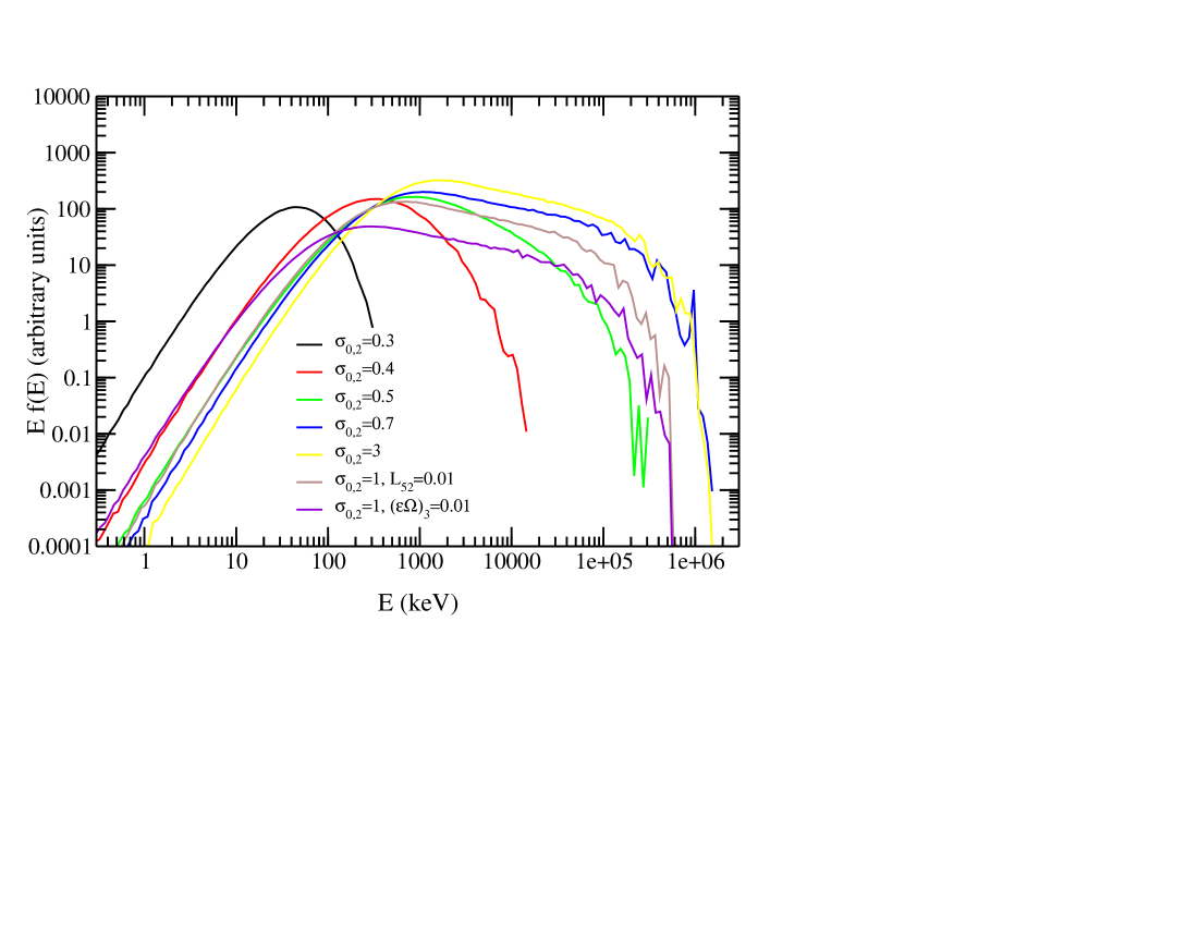
Figure 1: Photospheric spectrum of the reconnection model for GRB flows (photon energies in the central engine frame). For moderate and high initial Poynting flux ratio $\sigma_{0}$ the spectra peak around 1 MeV. The flat high energy tail is the result of inverse Compton scattering of photons off hot electrons close to the photospheric radius. For low $\sigma_{0}$ dissipation stops below the photosphere, and the resulting spectrum is quasi-thermal.

A selection of characteristic emergent spectra from the calculations are presented in Fig. 1 in $E\cdot f(E)$ representation for different values of the parameters of the model. The spectra are plotted in the central engine frame with arbitrary normalization (the energetics are discussed in the next Section). The peak of the spectrum is close to $\leavevmode\nobreak\ 1$ MeV for a large region of the parameter space which is relevant for GRB flows. The dependence of the peak energy on the parameters of the model is very weak. This can be understood from the fact that the peak energy is related to the peak of the thermal emission advected with the flow at the equilibrium radius which, in the central engine frame, is $E_{\rm p,th}\propto T_{\rm eq}^{\rm ce}\propto\Gamma(r_{\rm{eq}})T_{\rm th}(r_{\rm eq})\propto L_{52}^{1/9}(\varepsilon\Omega)_{3}^{1/3}\sigma_{0,2}^{1/3}$, where in the last step the expressions (9), (LABEL:gamma) and (10) have been used. The detailed numerical investigation leads to very similar dependence of $E_{\rm p}$ on the model parameters (see eq. 14).

The inverse Compton scattering that takes place above the equilibrium radius leads to a moderate increase of the energy of the peak and, most important, to a power-law high energy emission with photon number index $\sim-2.5$ that extends up to a few hundred MeV. This high energy part of the spectrum is the result of unsaturated Comptonization taking in the $\tau\mathbin{\lower 3.0pt\hbox{$\hbox to0.0pt{\raise 5.0pt\hbox{$\char 60\relax$}\hss}\mathchar 29208\relax$}}1$ region and appears for flows with $\sigma_{0}\mathbin{\lower 3.0pt\hbox{$\hbox to0.0pt{\raise 5.0pt\hbox{$\char 62\relax$}\hss}\mathchar 29208\relax$}}\sigma_{\rm 0,cr}$.

In the lower $\sigma_{0}$ cases, the emergent spectrum has much weaker emission above its peak. In these cases the magnetic dissipation stops below the Thomson photosphere and there is only weak Compton upscattering taking place in the photospheric region. Such quasi-thermal emission has been observed in a fraction of GRBs (Ryde 2004; 2005) suggesting these may be bursts of low $\sigma_{0}$ (high baryon loading).

3 Analytical fits and parametric study of the spectra

The spectra obtained with our Monte-Carlo radiative transfer calculations have systematic dependencies on the parameters of the model (initial Poynting flux to kinetic flux ratio $\sigma_{0}$, luminosity per steradian $L$ and reconnection rate which appears in the combination $\epsilon\Omega$). In this section we condense these dependences into a more practically useful form by developing fitting formulas.

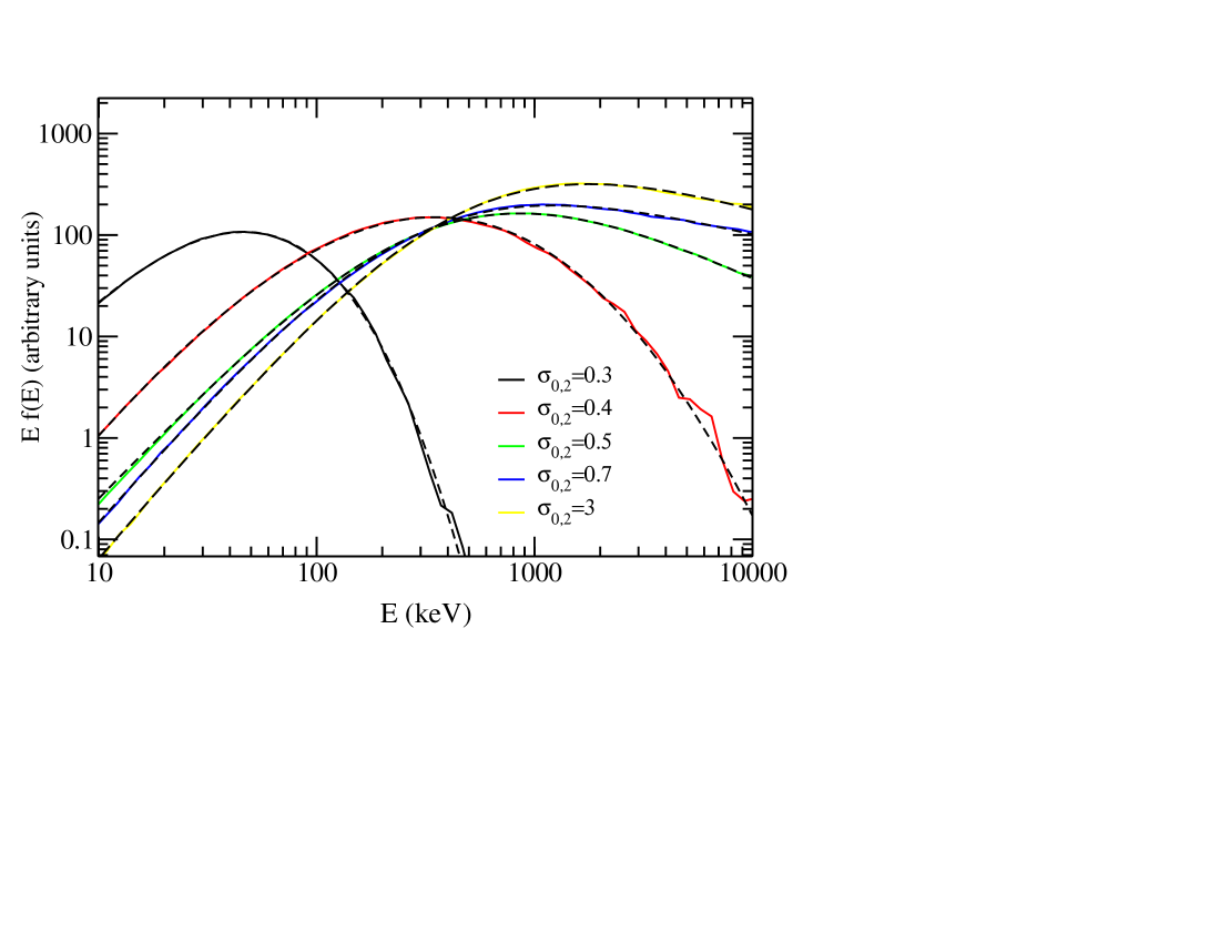
Figure 2: Smoothly-broken power law fits (dashed) to the spectra of Fig. 1 (solid). Photon energies in the central engine frame. The 5-parameter SBPL formula (eq. (11)) fits the numerically calculated spectra very accurately in the 10 keV to 10 MeV energy range.

After various attempts to find analytical functions that fit the numerically computed spectra, it turned out that the smoothly connected power law (hereafter SBPL model Preece et al. 1994; Ryde 1999; Kaneko et al. 2006) provides a very good description in the 10 keV to 10 MeV energy range, which is the most relevant for observations of the prompt emission of GRBs. The SBPL is a generalization of the sharply broken power law model by the addition of a parameter governing the width of the transition from the low energy spectral slope to the high energy slope. The fitting model has five parameters: an amplitude $A$, low and high photon indexes $\lambda_{1}$ and $\lambda_{2}$, a break energy $E_{\rm{b}}$ and a break scale $\Lambda$. The transition in slope is described by a hyperbolic tangent function.

The SBPL model fits the data (in our case the spectrum) with the expression (for the derivation see for example Ryde 1999)

$$f(E)=A\Big{(}\frac{E}{100}\Big{)}^{\frac{\lambda_{1}+\lambda_{2}+2}{2}}\Big{(}\frac{e^{q}+e^{-q}}{e^{q_{\rm piv}}+e^{-q_{\rm piv}}}\Big{)}^{\frac{\lambda_{2}-\lambda_{1}}{2}\Lambda},$$ (11)

where

$$q=\frac{\ln(E/E_{\rm b})}{\Lambda},\quad q_{\rm piv}=\frac{\ln(100/E_{\rm b})}{\Lambda}.$$

The amplitude $A$ is in photons $s^{-1}$ and all energies in keV.

The break energy $E_{\rm b}$ is related to the peak energy $E_{\rm p}$ of the distribution $Ef(E)$ by

$$E_{\rm p}=E_{\rm b}\Big{[}-{\lambda_{1}+2\over\lambda_{2}+2}\Big{]}^{\Lambda/2}$$ (12)

(e.g., Kaneko et al. 2006).

Since this fitting model does not have a high energy exponential break, it cannot describe the spectra above $\sim 100$ MeV. The SBPL fits also show small systematic deviations for energies below $\sim$several keV. Thus, we limit our fits to the, nevertheless broad, 10 KeV - 10 MeV energy range. We have used the SBPL model to fit a large number of theoretical spectra for models of varying luminosity $L$, baryon loading $\sigma_{0}$ and reconnection rate parameterized by $\varepsilon\Omega$.

A few, rather representative, examples of such fits are shown in Fig. 2. The fits (shown as dashed curves) lie very close to the numerical results with the exception of the lowest end of the energy range considered. Overall, SBPL fits are a very good way to summarize the photospheric spectrum predicted by the dissipation model.

With these fits, the low and high energy slopes $\lambda_{1}$ and $\lambda_{2}$ and the peak energy $E_{\rm p}$ of the spectrum can be presented as functions of the parameters of $L$, $\sigma_{0}$ and $\varepsilon\Omega$ of the model.

Fig. 3 shows the ratio of the photospheric emission to total flow luminosity, i.e. the (photospheric) radiative efficiency of the model and Fig. 4 the peak energy $E_{\rm p}$ of the spectrum. For $\sigma_{0}$ around the critical value $\sigma_{\rm 0,cr}$, the radiative efficiency peaks at $\approx 0.35f_{\rm e}$, independent of the luminosity of the flow $L$ and the reconnection rate parameter $\varepsilon\Omega$ . For $\sigma_{0}<\sigma_{\rm 0,cr}$, the magnetic dissipation stops below the photosphere and radiation suffers substantial adiabatic cooling before it decouples from matter; this results in a steep increase of the radiative efficiency and of the peak energy as functions of $\sigma_{\rm 0}$. Changes in $L$ and $\varepsilon\Omega$ lead to characteristic displacements of the curves in the $L_{\rm ph}/L-\sigma_{0}$ and $E_{\rm p}-\sigma_{0}$ planes (see Figs. 3 and 4).

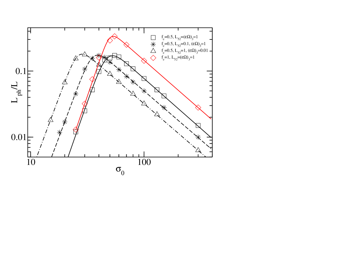
Figure 3: The (photospheric) radiative efficiency of the flow (ratio of photospheric luminosity to flow luminosity), as a function of the initial Poynting flux to kinetic energy flux ratio $\sigma_{0}$. At low $\sigma_{0}$, most of the dissipation happens at great optical depth, and the photospheric radiation field is reduced by adiabatic expansion. At high $\sigma_{0}$ most dissipation takes places beyond the photosphere. The solid red line shows the effect of increasing the electron fraction of the dissipated energy from 50 to 100%. Changes in luminosity $L$ and $\varepsilon\Omega$ are equivalent to shifts along the $\sigma$-axis. The curves are fits to smoothly broken power laws (best fit values in the appendix A.2).

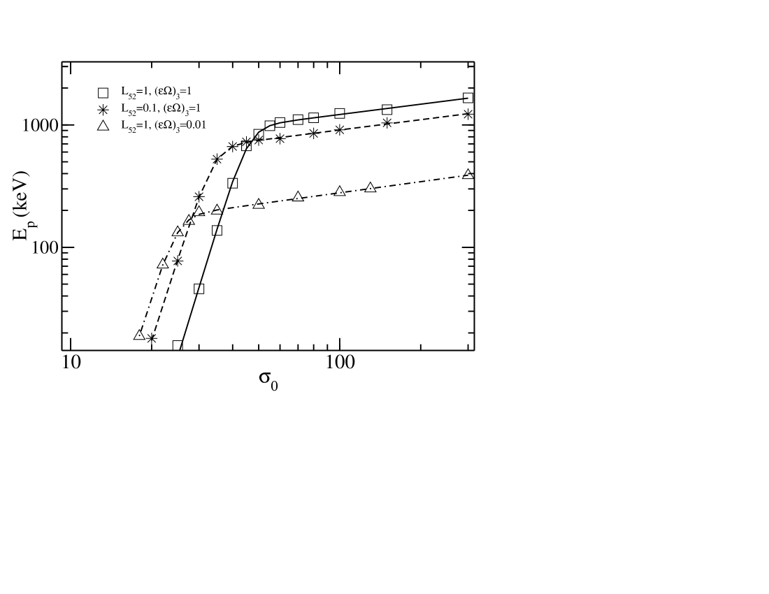
Figure 4: Dependence of peak energy (peak of the photospheric $E\cdot f(E)$ spectrum) on baryon loading, flow luminosity and reconnection speed. Above the characteristic Poynting flux parameter $\sigma_{0,{\rm cr}}$ (Eq. 7), $E_{\rm p}$ depends only weakly on baryon loading. At high baryon loading (low $\sigma_{0}$), the spectrum becomes quasithermal (cf. Fig. 1), peaking at a low energy. Curves show the smoothly broken power law fits (cf. appendix A.2).

Analytic fits for the radiative efficiency and peak energy as functions of the characteristics of the flow are given in the appendix. These expressions reduce to simple power laws when $\sigma\mathbin{\lower 3.0pt\hbox{$\hbox to0.0pt{\raise 5.0pt\hbox{$\char 62\relax$}\hss}\mathchar 29208\relax$}}\sigma_{\rm cr}$. Thus, for a sufficiantly high initial magnetization parameter in the flow, the radiative efficiency has the following dependence on the model parameters (see Sect. A.2)

$$L_{\rm ph}/L\approx 0.07\sigma_{0,2}^{-1.5}(\varepsilon\Omega)_{3}^{0.2}L_{52}^{0.2},\quad\sigma_{0}>\sigma_{\rm 0,cr}.$$ (13)

Similarly, for $\sigma_{0}>\sigma_{\rm 0,cr}$ the expression for the peak energy simplifies to (see Sect. A.3)

$$E_{\rm p}\approx 1200L_{52}^{0.11}(\varepsilon\Omega)_{3}^{0.33}\sigma_{0,2}^{0.3}\quad{\rm keV},\quad\sigma_{0}>\sigma_{\rm 0,cr}.$$ (14)

The high-energy photon index $\lambda_{2}$ is almost constant at $\sim-2.5$ for $\sigma_{0}\mathbin{\lower 3.0pt\hbox{$\hbox to0.0pt{\raise 5.0pt\hbox{$\char 62\relax$}\hss}\mathchar 29208\relax$}}\sigma_{\rm 0,cr}$ and decreases rapidly for smaller $\sigma_{0}$ (because there is little or no dissipation close to the photosphere for low values of $\sigma_{0}$). The expression for $\lambda_{2}$ as a function of the characteristics of the flow is given in the appendix A.4. The low-energy photon index $\lambda_{1}$ shows very small variations and remains approximately $\sim 0$ in most the parameter space investigated. For simplicity, we keep $\lambda_{1}=0$ independently of the characteristics of the flow. On the other hand, significant softening of $\lambda_{1}$ appears when the spectral peak approaches the lowest energy range over which the spectral fits are performed (i.e. at 10 keV). This may lead to deviations of the fitting formulas and the actual predictions of the photospheric model in the $\sim 10$ keV range (in the frame of the central engine). The break scale $\Lambda$ is practically constant $\sim 1.6$ for high $\sigma_{0}$ and makes a transition to the value $\sim 2.8$ for $\sigma_{0}<\sigma_{\rm 0,cr}$. This transition can be modeled by a hyperbolic tangent (see appendix A.2).

3.1 The non-photospheric emission

The spectra above were obtained with an outer boundary set at a scattering optical depth of 0.1. In the optically thin part of the flow ($\tau<0.1$) the electron temperature will continue to rise if significant dissipation takes place there, and this will contribute to the Comptonization. We have not included this contribution so far because the assumption of a thermalized electron distribution becomes questionable at $\tau\mathbin{\lower 3.0pt\hbox{$\hbox to0.0pt{\raise 5.0pt\hbox{$\char 60\relax$}\hss}\mathchar 29208\relax$}}0.1$, and a nonthermal distribution will change the Comptonization process. This makes the emission in these regions dependent on poorly known details of the magnetic dissipation process.

Notwithstanding this, it is possible to get an idea concerning at which energy band the optically thin emission may be expected to take place by extending the outer boundary of the Monte Carlo calculation to larger radii (or equivalently to smaller optical depths in the flow). In this excercise we assume that the electrons still follow a thermal distribution in this region. In Fig. (5) the emitted spectrum for the reference values of the parameters of the model is shown for various values of the optical depth $\tau_{\rm out}$ at the outer boundary of the numerical calculation. The spectrum below the peak energy remains essentially the same. The higher energy emission is significantly enhanced as a result of scattering in the very hot, optically thin part of the flow. The high-energy spectral slope hardens, approaching $\lambda_{2}\sim-2$, and there is substantial emission in the $\sim$GeV energy range.

The vertical dashed lines show the energy range used for the fitting formulas presented in the previous section. The optically thin emission affects the high-energy spectral slope $\lambda_{2}$ somewhat, which now lies in the $\sim-2$ to $-2.5$ range. The optically thin emission increases the luminosity in the 10-1000keV range only moderately, but can produce a significant peak in the GeV range.

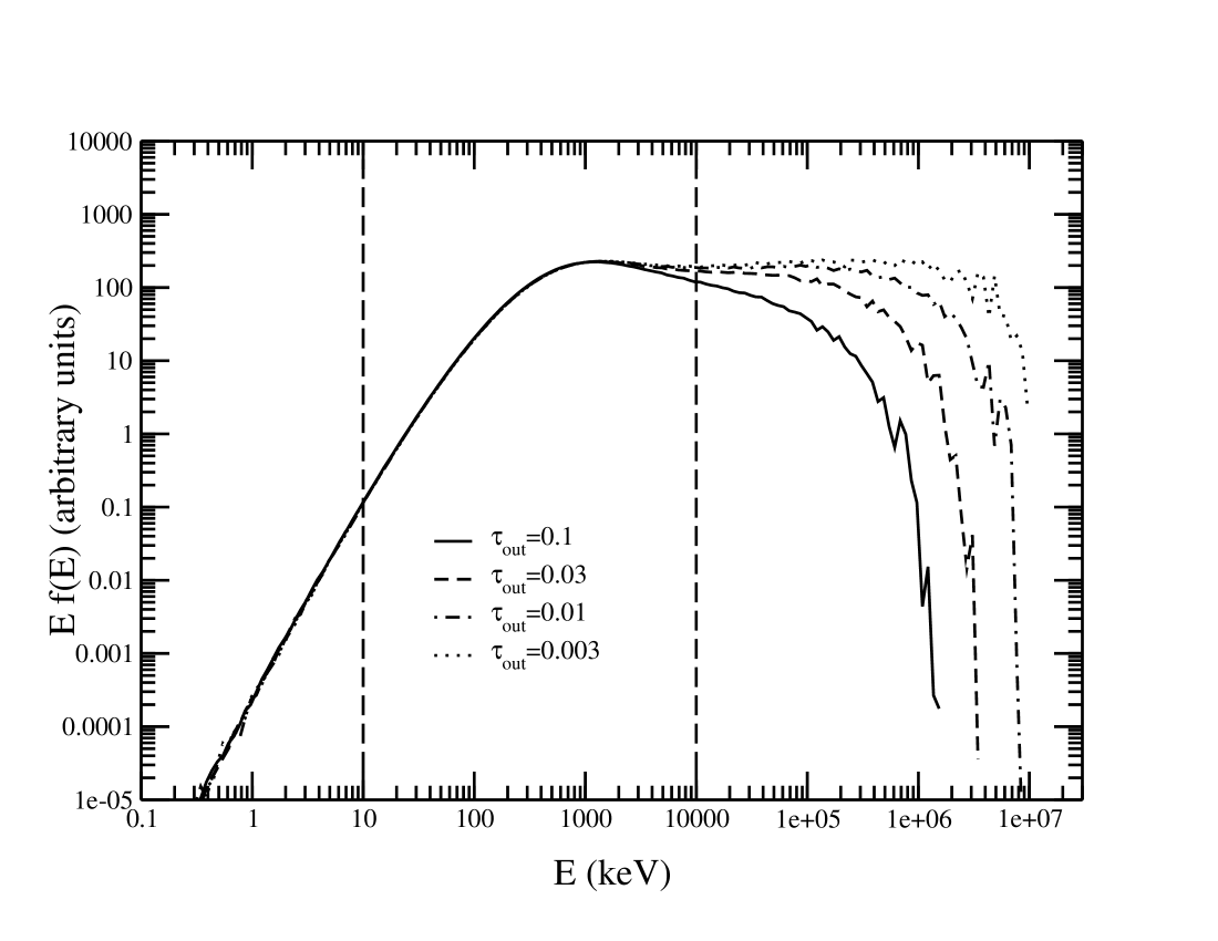
Figure 5: Modification of the spectrum when an estimate of the emission in the optically thin part of the flow is included. [Electron distribution is assumed to remain thermal at low optical depths.] Parameter is the optical depth at the outer boundary of the calculation (photon energies in the central engine frame). Dashed lines mark the range used for the fitting formulas.

4 Interpretation of the observations

In the following we use a first comparison with observations to make inferences about the properties of GRB outflows in the magnetic dissipation model.

4.1 The value of $E_{\rm p}$

The observed spectral peak of the prompt emission spectrum of GRBs has a narrow distribution peaking at $\sim$250 keV (Band et al. 1993; Kaneko et al. 2006); by far the largest amount of data emanates from BATSE. To compare this distribution with the prediction of the photospheric model (14) the redshift distribution of GRBs has to be taken into account. This distribution is not well known for the BATSE bursts, but various estimates indicate that an average value of $z\sim 1.5-2$ is reasonable. For a typical burst at this redshift the model predicts that (cf. eq. (14))

$$E_{\rm p}^{\rm obs}=\frac{E_{\rm p}}{1+z}\simeq 450L_{52}^{0.11}(\varepsilon\Omega)_{3}^{0.33}\sigma_{0,2}^{0.3}\quad{\rm keV}.$$ (15)

The dependence on the characteristics of the flow is weak; the model thus predicts a narrow distribution of the peak energy of bursts, in agreement with observation. For the reference values of the parameters used in eq. (15), the peak energy predicted by the model is at 450 keV, a factor of $\sim 2$ above the value for BATSE bursts. Though this is not a large factor, the weak dependence on model parameters implies a significant difference in one or more of them compared with the reference value. A low value for $\sigma_{0}\ll 100$ is not attractive, since then the flow becomes too slow to explain the typical GRB. The very weak dependence of the peak energy on the luminosity also excludes the burst luminosity. Since the central engine is most likely a stellar mass compact object, the rotation rate, $\Omega$, must be of the order $10^{3}-10^{4}$ rad s^-1. The most uncertain parameter of the magnetic dissipation model is actually the reconnection speed parameter $\varepsilon$, for which we have so far assumed a value $\sim 0.1$ (Drenkhahn 2002). $\Omega=10^{4}$ rad s^-1 is perhaps on the high side for the torus in a collapsar, and $\varepsilon=0.1$ possibly too optimistic. A value $(\varepsilon\Omega)\sim 100$ rad s^-1 instead of $10^{3}$, which would bring the predicted value of $E_{\rm p}$ into agreement with observation, can easily be accommodated within these uncertainties.

This indicates that magnetic dissipation timescale is one order of magnitude longer than that assumed by the reference values of the parameters. In the following we adopt $(\varepsilon\Omega)=10^{2}(\varepsilon\Omega)_{2}$ as a reference value for the parameterization of the dissipation timescale.

4.2 The Amati relation

There are indications in the literature that the peak energy $E_{\rm p}$ of a burst correlates with the isotropic equivalent energy: $E_{\rm p}\propto E_{\rm iso}^{0.5}$ (Amati et al. 2002; Amati 2006), although this correlation is probably not universal (Nakar& Piran 2005; Band & Preece 2005). The isotropic equivalent energy of the prompt emission is $E_{\rm iso}\sim L_{\rm ph}t_{\rm GRB}$, where $t_{\rm GRB}$ is the duration of the burst. For an estimate of the energy of the prompt emission, the relevant luminosity is that of the photosphere $L_{\rm ph}$ and not that of the flow $L$.

Using the expressions (14) and (13) one can find the dependence on the parameters of the flow of the ratio

$$\frac{E_{\rm iso}^{1/2}}{E_{\rm p}}\propto\frac{L^{0.5}t_{\rm GRB}^{0.5}}{(\varepsilon\Omega)^{0.23}\sigma_{0}^{1.1}}.$$ (16)

According to the Amati relation, this ratio stays approximately constant over a wide range of $E_{\rm iso}$. Since the dispersion in the distribution of durations of $t_{\rm GRB}^{1/2}$ for long GRBs is rather small $\sim 10^{1/2}$, it is unlikely that a dependence in a systematic way of $t_{\rm GRB}$ with another parameter (say the luminosity) is responsible for keeping the ratio (16) constant. On the other hand, the ratio is approximately constant for $\sigma_{0}\propto L^{\sim 0.4-0.5}$ in different bursts. The Amati relation, therefore, indicates that there is a corelation of baryon loading and luminosity, in the sense that the most luminous GRB flows have more energy per baryon. We see in the next Section that if the same baryon loading-luminosity corelation holds during the evolution of individual GRBs, the model predicts the observed energy dependence of the width of pulses in the GRB lightcurves.

4.3 GRB variability and spectral evolution

Up this point, we have dealt with a steady flow that is characterized by fixed luminosity and baryon loading. This approach can, to some extent, describe the rough, time average, properties of a GRB. On the other hand, the GRB lightcurves are highly variable and are composed by a sequence of pulses believed to be the “building blocks” of their lightcurves (e.g. Fenimore et al. 1995). The question that rises as to where the variability comes from in the photospheric model for the prompt emission and under what conditions a steady state model such as the magnetic reconnection one can describe a variable flow.

An ultrarelativistic flow that varies on a timescale $\delta t$ can be still described by a steady state model as long as $\delta t>r/\Gamma^{2}c$. When the last condition holds, the leading and trailing parts of a piece of the flow with width $\delta r\simeq c\delta t$ have not come into causal contact. As long as this is the case, different parts of the flow behave as part of a steady wind. A robust proof of this statement can be found in Piran et al. (1993) for fireballs and Vlahakis & Königl (2003) for MHD flows. The relevant radius of interest in this study is the photospheric radius. As far as the photospheric emission is concerned, the steady state approximation is valid for a flow which varies on timescales

$$\delta t>\frac{r_{\rm ph}}{\Gamma^{2}(r_{\rm ph})c}\simeq 2\cdot 10^{-3}\frac{L_{52}^{1/5}}{(\varepsilon\Omega)_{2}^{4/5}\sigma_{0,2}^{3/2}}\quad{\rm s},$$ (17)

where eqs. (7) and (LABEL:gamma) are used in the last step. The flow can treated as approximately steady for all but the shortest observed (sub-millisecond) timescales.

4.3.1 Central engine: the stronger the cleaner

Variability and dissipation are, a priori, unrelated in the magnetic reconnection model in which dissipation takes place, even in a steady magnetic outflow. On the other hand, the flow does evidently evolve during a GRB. In the context of the present model, the observed variability reflects changes in the luminosity (and possibly the initial magnetization parameter or even the reconnection rate $\varepsilon\Omega$) during the burst. Since the flow up to the photosphere can be treated as quasi-stationary for all but the shortest time scales observed in a burst, the variation of spectral properties during a burst directly reflects variations in the central engine. This is in contrast to models in which the prompt radiation is produced at much larger distances from the source, such as external shock models. It is also in contrast with the internal shock model, since the internal evolution of the flow between the source and the level where radiation is emitted is a key ingredient in this model. Deducing properties of the central engine from observed burst properties is thus a much more direct prospect in the magnetic dissipation model.

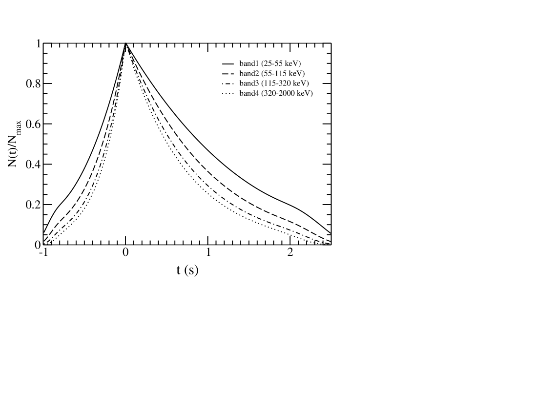
Figure 6: Narrowing of pulse width with photon energy, as predicted by the model for individual subpulses of the burst. The assumption is that the relation between luminosity and baryon loading deduced from the Amati relation, $\sigma_{0}\propto L^{0.4}$, holds also within a burst.

As a first application we consider here the width of subpulses in a burst. The observations show this width to be a decreasing function of photon energy (e.g. Fenimore et al. 1995). GRBs with complex light curves (composed of many subpulses) follow the same Amati relation as simple ones (with one or a few pulses). In the above, we have shown how this relation implies a dependence of the baryon loading of the burst on its luminosity. We now make the logical extrapolation of assuming that this same relation also holds for the time-dependent flow during a burst. Varying the luminosity of the flow with time in such a way that it mimics the typical pulse profile, one can simulate the pulse appearance predicted by the photospheric model in different energy bands. To reproduce the characteristic pulse shape, we consider time dependence of the luminosity of the flow of the form (cf. Norris et al. 1996)

$$L(t) = L_{\rm max}e^{-|t/t_{\rm r}|},\quad t<0$$

$$L(t) = L_{\rm max}e^{-t/t_{\rm d}},\quad t>0$$

where $t_{\rm r}=0.2/(1+z)$ s and $t_{\rm d}=0.5/(1+z)$ s are the rise and decay timescales of the lightcurve (in the central engine frame) respectively and $L_{\rm max}=10^{52}$ erg s^-1 sterad^-1. We also assume that the baryon loading tracks the luminosity with the expression $\sigma_{0,2}=L_{52}^{0.4}$ (indicated by the Amati relation) and set $\varepsilon\Omega=100$ rad s^-1. The redshift of the burst, needed to correct for photon reshifting and cosmological time dilation, is taken to be $z=2$.

Having specified the parameteres of the flow as functions of time, one can calculate the lightcurve (in the observer’s frame) of the photopsheric emission at different energy bands predicted by the photospheric model using eq. (11) and the expressions in the appendix. In fig. 6, the predicted lightcurves in the BATSE energy bands are plotted. The lightcurves of the harder energy bands are narrower than those of the softer. The width in the 320-2000 keV band being approximately half of that of the 25-55 keV band close to what is observed. The energy dependence of the lightcurves comes from the spectral hardening of the photospheric emission with increasing luminosity $L$ (and therefore increasing photospheric luminosity $L_{\rm ph}$; see eqs. (13) and (14)). This spectral hardening results in relatively enhanced emission in the hard bands (with respect to the softer ones) when the luminosity is close to its peak.

5 Discussion/conclusions

In the magnetic reconnection model, the flow that powers a GRB is initially Poynting flux dominated. The model is characterized by gradual dissipation of magnetic energy that leads to acceleration of the flow and an increase in its internal energy. For characteristics of the flow typical to those expected for GRB flows (i.e., high luminosities and low baryon loadings) the dissipation continues at distances outside the point where the flow becomes transparent with respect to Thomson scattering (i.e. outside the Thomson photosphere). The energy release close to the photospheric radius leads to a hot photosphere. Inverse Compton scattering of the advected with the flow photon field by hot electrons leads to photospheric spectra with a characteristic non-thermal appearance and with peak energy and spectral slopes close to those observed in the prompt phase of GRBs. The radiative transfer problem has been studied in detail, with both analytical and numerical tools, in G06.

Here, we build further on that study by providing an accurate analytical description of the spectra predicted by the model in the x-ray and $\gamma$-ray regime. We show that the photospheric emission from the reconnection model is well described by a smoothly broken power law model. Simple fitting formulas are presented for the bolometric luminosity and peak energy of the $E\cdot f(E)$ spectrum as a function of the flow parameters (i.e. the luminosity of the flow $L$, the baryon loading $\sigma_{0}$ and the reconnection timescale parameter $\varepsilon\Omega$).

The model predicts the observed clustering of the peak energy of the $E\cdot f(E)$ spectrum in the sub-MeV range and its quantitative comparison with observations indicates that the combination of parameters $(\varepsilon\Omega)$ (where $\varepsilon$ stands for the fraction of the Alfvén speed with which reconnection takes place and $\Omega$ for the angular frequency of the rotator) has values $(\varepsilon\Omega)\sim 100$ rad s^-1. This is compatible with reconnection speed proceeding with $\varepsilon\sim 0.03$ and a rotator with angular frequency $\Omega\sim 10^{3.5}$rad s^-1. The Amati relation (i.e. $E_{\rm p}\sim E_{\rm iso}^{0.5}$; Amati et al. 2002; 2006) can be explained by the model provided that the most luminous bursts are characterized by higher energy-to-rest-mass ratio.

More constraints to both the model and the operation of the central engine can come from the study of the variability properties of the GRBs. In the photospheric model, the observed variability is a direct manifestation of the activity of the central engine. Individual pulses, considered to be the building blocks of the GRB lightcurves (e.g. Fenimore et al. 1995) come from modulations of the luminosity and the baryon loading of the flow and are ultimately linked to the central engine variability. Modeling of the observed properties of the GRB pulses can, thus, provide us with a unique probe into oparation of the central engine on diferent timescales during the GRB prompt phase.

We have simulated GRB pulses by assuming that the luminosity of the flow varies following the typical observed pulse profile (cf. Norris et al. 1996) and that the magnetization parameter $\sigma_{0}$ corelates with the luminosity of the flow as indicated by our interpretation of the Amati relation. The pulse width predicted by the model is narrower in the harder energy bands, in agreement with observation.

Appendix A Fitting functions for the spectral parameters

Here we give the expressions that describe how the photospheric luminosity $L_{\rm ph}$, the peak energy $E_{\rm p}$, the high frequency power law $\lambda_{2}$ and the spectral break $\Lambda$ depend on the physical parameters $L$, $\sigma_{0}$ and $\varepsilon\Omega$ of the reconnection model. We first, derive some useful expressions related to the SBPL model that will simplify the apearance of the fitting formulas.

A.1 A note on the Smoothly connected power-law model

The expression that describes the SBPL model can be quite generally written (e.g., Ryde 1999)

$$g(x)=A\Big{(}\frac{x}{x_{\rm piv}}\Big{)}^{\frac{\lambda_{1}+\lambda_{2}}{2}}\Big{(}\frac{e^{q}+e^{-q}}{e^{q_{\rm piv}}+e^{-q_{\rm piv}}}\Big{)}^{\frac{\lambda_{2}-\lambda_{1}}{2}\Lambda},$$ (19)

where

$$q=\frac{\ln(x/x_{\rm b})}{\Lambda},\quad q_{\rm piv}=\frac{\ln(x_{\rm piv}/x_{\rm b})}{\Lambda}.$$

The value $x_{\rm piv}$ is a reference value of the $x$ variable one has the freedom to choose. For $x=x_{\rm piv}$ one easily check that $g(x_{\rm piv})=A$.

This expression can be simplified if the reference value $x_{\rm piv}$ is taken sufficiently far from the break $x_{\rm b}$. If, for example, $e^{q_{\rm{piv}}}\gg e^{-q_{\rm{piv}}}$, one can simplify the expression for the SBPL model.

Under the condition that $e^{q_{\rm{piv}}}\gg e^{-q_{\rm{piv}}}$ eq. (19) can be brought into the form

$$g(x)=A\Big{(}\frac{x}{x_{\rm piv}}\Big{)}^{\frac{\lambda_{1}+\lambda_{2}}{2}}\Big{(}\frac{x_{\rm b}}{x_{\rm piv}}\Big{)}^{\frac{\lambda_{2}-\lambda_{1}}{2}}\Big{(}e^{q}+e^{-q}\Big{)}^{\frac{\lambda_{2}-\lambda_{1}}{2}\Lambda}.$$ (20)

One can also derive the asymptotic expressions for the low and high power-law dependence of $g(x)$ on $x$ in the limits $e^{q}\gg e^{-q}$ and vice versa. So expression (20) gives

$$g(x)=A\Big{(}\frac{x}{x_{\rm piv}}\Big{)}^{\lambda_{2}},\quad e^{q}\gg e^{-q}$$ (21)

and

$$g(x)=A\Big{(}\frac{x}{x_{\rm piv}}\Big{)}^{\lambda_{1}}\Big{(}\frac{x_{\rm b}}{x_{\rm piv}}\Big{)}^{\lambda_{2}-\lambda_{1}},\quad e^{q}\ll e^{-q}.$$ (22)

The form (20) of the SBPL model is used below for fitting the dependency of the photospheric spectrum on the parameters of our magnetically powered GRB flow.

A.2 Fitting formulas

The dependency of the photospheric bolometric luminosity on $\sigma_{0}$ is well modeled by a SBPL model (see fig. 3) of the form

$$L_{\rm ph}=A_{\rm L}\Big{(}\frac{\sigma_{0}}{100}\Big{)}^{1.5}\Big{(}\frac{\sigma_{\rm 0,cr}}{100}\Big{)}^{-3}\Big{(}e^{q}+e^{-q}\Big{)}^{-0.5},$$ (23)

where

$$q=6\ln(\sigma_{0}/\sigma_{\rm 0,cr})$$

and $\sigma_{\rm 0,cr}=42\big{(}L_{52}(\varepsilon\Omega)_{3}\big{)}^{2/15}$ (defined in eq. (8)). The best fit for $A_{\rm L}$ is

$$A_{\rm L}\approx 7\cdot 10^{50}(\varepsilon\Omega)_{3}^{0.2}L_{52}^{1.2}\quad\rm{erg\cdot s^{-1}}.$$ (24)

The rather sharp break means that for $\sigma_{0}>\sigma_{\rm 0,cr}$ the photospheric luminosity is well represented by (see also eq. (21))

$$L_{\rm ph}=7\cdot 10^{50}(\varepsilon\Omega)_{3}^{0.2}L_{52}^{1.2}\sigma_{0,2}^{-1.5}\quad\rm{erg\cdot s^{-1}}.\qquad(\sigma>\sigma_{0})$$ (25)

The fit for the peak energy of the $E\cdot f(E)$ spectrum on $\sigma_{0}$ is

$$E_{\rm p}=A_{\rm p}\Big{(}\frac{\sigma_{0}}{100}\Big{)}^{3.6}\Big{(}\frac{\sigma_{\rm 0,cr}}{100}\Big{)}^{-3.3}\Big{(}e^{q}+e^{-q}\Big{)}^{-0.55},$$ (26)

with

$$A_{\rm p}\approx 1200(\varepsilon\Omega)_{3}^{0.33}L_{52}^{0.11}\quad{\rm keV}.$$ (27)

For $\sigma_{0}>\sigma_{\rm 0,cr}$ this reduces to (cf. eq. (21))

$$E_{\rm p}\approx 1200(\varepsilon\Omega)_{3}^{0.33}L_{52}^{0.11}\sigma_{0,2}^{0.3}\quad{\rm keV}.$$ (28)

The fit for the high-energy slope is

$$\lambda_{2}\approx-2.5\Big{(}\frac{\sigma_{0}}{100}\Big{)}^{-1.8}\Big{(}\frac{\sigma_{\rm 0,cr}}{100}\Big{)}^{1.8}\Big{(}e^{q}+e^{-q}\Big{)}^{0.3}.$$ (29)

The break scale is approximately constant, $\Lambda\simeq 1.6$, for high $\sigma_{0}$ and makes a transition to $\Lambda\simeq 2.8$ for low values of $\sigma_{0}$. The transition is modeled with the hyperbolic tangent function with best fit

$$\Lambda\approx 2.2-0.6\tanh\Big{(}8\frac{\sigma_{0}-\sigma_{0,{\rm cr}}}{\sigma_{0,{\rm cr}}}\Big{)}.$$ (30)

An approximation to the spectrum itself, as a function of baryon loading, flow luminosity and reconnection rate, is given by eq. (11), with parameters given by the fitting formulas above. The normalization factor $A$ in eq. (11) follows by equating the integrated luminosity $\int f(E)\,{\rm d}E$ to the photospheric luminosity from 23.

References

- (1) Abramowicz, M. A., Novikov, I. D., & Paczyński, B. 1991, ApJ, 369, 175
- (2) Amati, L., Frontera, F., Tavani, M., et al. 2002, A&A, 390, 81
- (3) Amati, L. 2006, MNRAS, 372, 233
- (4) Band, D., & Preece, R. D. 2005, ApJ, 627, 319
- (5) Band, D., Matteson, J., Ford, L., et al. 1993, ApJ, 413, 281
- (6) Blandford, R. D., & Payne, D. G. 1982, MNRAS, 199, 883
- (7) Coroniti, F. V. 1990, ApJ, 349, 538
- (8) Crider, A., Liang, E. P., Smith, I. A., et al. 1997, ApJ, 479, L39
- (9) Daigne, F., & Mochkovitch, R. 2002, MNRAS, 336, 1271
- (10) Drenkhahn, G. 2002, A&A, 387, 714
- (11) Drenkhahn, G., & Spruit, H. C. 2002, A&A, 391, 1141
- (12) Fenimore, E. E., in ’t Zand, J. J. M., Norris, J. P., Bonnell, J. T., & Nemiroff, R. J. 1995, ApJ, 448, L101
- (13) Frontera, F., Amati, L., Costa, E., et al. 2000, ApJS, 127, 59
- (14) Ghirlanda, G., Celotti, A., & Ghisellini, G. 2003, A&A, 406, 879
- (15) Ghisellini, G., & Celotti, A. 1999, A&AS, 138, 527
- (16) Giannios, D. 2006, A&A, 457, 763
- (17) Giannios, D., & Spruit, H. C. 2005, A&A, 430, 1
- (18) Giannios, D., & Spruit, H. C. 2006, A&A, 450, 887
- (19) Goodman, J. 1986, ApJ, 308, L47
- (20) Kaneko, Y., Preece, R. D., Briggs, M. S., et al. 2006, ApJS, 166, 298
- (21) Lyubarsky, Y. E. 2005, MNRAS, 358, 113
- (22) Lyutikov, M., & Blandford R. D. 2003, astro-ph/0312347
- (23) Mészáros, P., & Rees, M. J. 1997, ApJ, 482, L29
- (24) Mészáros, P., & Rees, M. J. 2000, ApJ, 530, 292
- (25) Michel, F. C. 1969, ApJ, 158, 727
- (26) Nakar, E., & Piran, T. 2005, MNRAS, 360, L73
- (27) Norris, J. P., Nemiroff, R. J., Bonnell, J. T., et al. 1996, ApJ, 459, 393
- (28) Paczyński, B. 1986, ApJ, 308, L43
- (29) Pe’er, A., Mészáros, P., & Rees, M. J. 2005, ApJ, 635, 476
- (30) Piran, T. 2005, Rev. Mod. Phys., 76, 1143
- (31) Piran, T., Shemi, A., & Narayan, R. 1993, MNRAS, 263, 861
- (32) Preece, R. D., Briggs, M. S., Mallozzi, R. S, & Brock, M. N. 1994, “WINdows Gamma SPectral ANalysis (WINGSPAN)”
- (33) Preece, R. D., Briggs, M. S., Mallozzi, R. S, et al. 1998, ApJ, 506, L23
- (34) Ramirez-Ruiz, E. 2005, MNRAS, 363, L61
- (35) Rees, M. J., & Mészáros, P. 1994, ApJ, 430, L93
- (36) Ryde, F. 1999, Astroph. Lett. and Comm., 39, 281
- (37) Ryde, F. 2004, ApJ, 614, 827
- (38) Ryde, F. 2005, ApJ, 625, L95
- (39) Sari, R., & Piran, T. 1997, MNRAS, 287, 110
- (40) Spruit, H. C., & Drenkhahn, G. D. 2004, Magnetically powered prompt radiation and flow acceleration in GRB, in Proceedings “Gamma Ray Bursts in the Afterglow Era, Third Workshop”, Rome, Sept 2002. ASP Conference Proccedings, 312, 357
- (41) Spruit, H. C., Daigne, F., & Drenkhahn, G. 2001, A&A, 369, 694
- (42) Thompson, C. 1994, MNRAS, 270, 480
- (43) Thompson, C., Mészáros, P., & Rees, M. J. 2006, ApJ, submitted, astro-ph/0608282
- (44) Uzdensky, D. A., & MacFadyen, A. I. 2006, ApJ, 647, 1192
- (45) Vlahakis, N., & Königl, A. 2003, ApJ, 596, 1080