Estimation of time delays from unresolved photometry

Abstract

Context. Longtime monitoring of gravitational lens systems is often done using telescopes and recording equipment with modest resolution. Still, it would be interesting to get as much information as possible from the measured lightcurves. From high resolution images we know that the recorded quasar images are often blends and that the corresponding time series are not pure shifted replicas of the source variability.

Aims. In this paper we will develop an algorithm to unscramble this kind of blended data.

Methods. The proposed method is based on a simple idea. We use one of the photometric curves, which is supposedly a simple shifted replica of the source curve, to build different artificial combined curves. Then we compare these artificial curves with the blended curves. Proper solutions for a full set of time delays are then obtained by varying free input parameters and estimating statistical distances between the artificial and blended curves.

Results. We performed a check of feasibility and applicability of the new algorithm. For numerically generated data sets the time delay systems were recovered for a wide range of setups. Application of the new algorithm to the classical double quasar QSO 0957+561 A,B lightcurves shows a clear splitting of one of the images. This is an unexpected result and extremely interesting, especially in the context of the recent controversy about the exact time delay value for the system.

Conclusions. The proposed method allows us to properly analyse the data from low resolution observations that have long time coverages. There are a number of gravitational lens monitoring programmes that can make use of the new algorithm.

1 Introduction

Gravitationally lensed quasar images can be monitored for a long period of time. The obtained time series can then be used to estimate time delays for different light paths to the observer. The best example of this kind of long-term photometry is a time series obtained by R. Schild and collaborators (see for instance Schild et al. Schild (1997)) for the ubiquitous system QSO 0957+561. Typically, such long programmes can be carried out only on small telescopes and consequently they will have a modest resolution. For many interesting multiply lensed systems, some of the images may remain unresolved. It occurs that for a reasonably long time series it is possible to recover complex time delay systems even from the blended images.

There are a number of different time delay estimation methods used by various research groups. For a short review of the popular methods see for instance Kundic̀ et al. (Kundic (1997)). Some recent more peculiar approaches can be found in Hjorth (Hjorth (1992)), Pijpers (Pijpers (1997)), Barkana (Barkana (1997)), Burud (Burud (2001)), and Gil-Merino (GilMerino (2002)). These methods can roughly be divided into three classes:

• cross-correlation based methods;

• methods based on interpolation (linear, polynomial, spline, etc.);

• methods which use dispersion spectra.

In principle, nearly all the known methods can be reformulated so that they can handle more complex models of time series, such as those treated in the current paper. Because of the simplicity and familiarity of the last class of methods, the new methods described hereafter are also based on the computing of dispersion spectra, introduced in Pelt et al. (Pelt94 (1994)) and refined in Pelt et al. (Pelt96 (1996)).

In Pelt et al. (Pelt98 (1998)), dispersion analysis was generalised for systems with multiple images. However, in previous papers and algorithms it was always assumed that observed curves are time-shifted replicas (perhaps distorted by microlensing) of the source variability. In practice, especially if we deal with low resolution photometry, this is not always the case. Often the photometric aperture covers several weak images and what we effectively get is the blend of different lightcurves. From physical considerations we can predict that the components of the blends are certain weighted sums of the time-shifted source variability curves. Typically, the time delays between blended components are remarkably shorter than the delays between images, which are significantly separated. A singular case of blending, where we observe only the sum of multiple components, was analysed in Geiger (Geiger (1996)). In this method a certain amount of extra information is used from additional interferometric observations.

Our paper is organised as follows. First we introduce general ideas of the proposed new algorithms. Then we formulate the algorithms in the terms of the specific time series operations involved. In the next part we describe the numerical tests we made to evaluate the algorithms. Then we consider applicability of the method in different contexts and apply the method to a real observed data sequence – the classical system QSO 0957+561 A,B. It is well known (from radio observations and deep images) that the photometric sequences for this system are not blends. However, as will be shown below, one of the observed curves can be disentangled into two quite clearly shifted source curves. Why it is so we do not know yet, but it is not ruled out that the well-known “small delay difference” controversy may be connected with this effect (see Yonehara Yonehara01 (1999); Gil-Merino et al. GilMerino01 (2001); Goicoechea Goicoechea (2002); Yonehara et al. Yonehara02 (2003)). Finally, we give a few recommendations for observers on how to plan long monitoring programmes for not fully resolved images.

2 Method

Here we use a slightly different formalism to introduce the new method (cf. original introduction of dispersion spectra in Pelt et al. (Pelt94 (1994, 1996))). In general, the source quasar image in a gravitational lens system is split due to the gravitational field of the intervening galaxy into multiple images $f_{1},\dots,f_{K}$. The source variability $q(t)$ shows itself in the measured lightcurves. Because of different flight paths the total flight times $t_{k},k=1,\dots,K$ differ. Consequently, the observed luminosities can be described as shifted (and possibly magnified) functions of the source variability $f_{k}(t)=a_{k}q(t-t_{k})$. For a fully resolved case we will have in total $K$ continuous curves $f_{k}(t)$. This somewhat oversimplified model ignores microlensing effects (variability of the magnification coefficients $a_{k}$ in time) and also other possible distortions. For each pair of images $f_{i},f_{j}$ we have the corresponding time delay $\Delta t_{i,j}=t_{j}-t_{i}$. From $N(N-1)/2$ delays only $N-1$ can be considered as independent. If we know all these independent delays, we can talk about a full set of time delays.

2.1 Two fully resolved lightcurves

Let us have two unblended images $f_{1}(t)=a_{1}q(t-t_{1})$ and $f_{2}(t)=a_{2}q(t-t_{2})$. We can shift the second curve by a time delay $\Delta t$ and multiply it by an arbitrary magnification ratio $a$ to form a difference $d(t)$

$$d(t,\Delta t,a)=f_{1}(t)-af_{2}(t+\Delta t).$$ (1)

If it happens that $\Delta t=\Delta t_{1,2}=t_{2}-t_{1}$ and $a=a_{1}/a_{2}$ then the difference vanishes, $d(t,\Delta t,a)=0$, and we say that the two curves match each other. In the case of noisy curves the match cannot be perfect. However, we expect that the dispersion of the difference is minimised for proper parameter values.

Finally, for discrete measurement series, we can hope that for each set of trial parameter values there are at least some time point pairs that can be used to estimate the dispersion. This dispersion is used then as a merit function to compare different combinations of parameters. This simple example shows that we can start from continuous curve models to build (using free parameters) matching pairs and then translate our algorithm into language of dispersion spectra. For the details of the method see Pelt (Pelt96 (1996)).

2.2 More than two fully resolved lightcurves

Sometimes we may have more than two fully resolved images and corresponding lightcurves (see Pelt Pelt98 (1998)). Just for simplicity let us look at a case when we have three images $f_{1}(t)=a_{1}q(t-t_{1})$, $f_{2}(t)=a_{2}q(t-t_{2})$, and $f_{3}(t)=a_{3}q(t-t_{3})$. Now we have three amplifications and three time delays from which only two are independent. There are also three different possibilities to match curves. As shown in Pelt (Pelt98 (1998)) it is reasonable to add dispersions from all three matches. This allows us to use information maximally in the sampled and noisy curves. The number of independent variables in this case is four – two delays and two amplification ratios.

2.3 A clean image and a blend

For three images we have basically only one interesting scheme with blended images. In this case we can observe one pure image, say $f_{1}(t)$ and one blend $f(t)=f_{2}(t)+f_{3}(t)=a_{2}q(t-t_{2})+a_{3}q(t-t_{3})$. These curves cannot be matched. However, we can use a “clean” curve $f_{1}(t)=a_{1}q(t-t_{1})$ to build an artificial blend curve $g(t)=f_{1}(t)+\alpha f_{1}(t-\Delta_{s})$, where $\alpha$ and $\Delta_{s}$ are additional free parameters to be determined. In the terms of the source curve we get $g(t)=a_{1}q(t-t_{1})+\alpha a_{1}q(t-t_{1}-\Delta_{s})$. It is not hard to see that in a fortunate case when $\Delta_{s}=\Delta t_{2,3}$ and $\alpha=a_{3}/a_{2}$, the curves $f(t)$ and $g(t)$ are shifted and amplified versions of each other and can be matched. Then we will have three parameters to vary: the two artificial blend parameters $\alpha$, $\Delta_{s}$ and the matching parameter $\Delta_{l}=\Delta t_{1,2}=t_{2}-t_{1}$. In the matching process we also estimate (for every parameter triple) two additional regression parameters: $a$ and $b$, which are discussed briefly in Sect. 2.5. As we see, in addition to subtraction (to match curves), we must also know how to add discretely sampled curves to build artificial blends.

2.4 Two blends

If we have four images, then there are many possibilities. The unblended scheme can be treated similarly to the case of three images. The only difference is that the combined dispersion has to be estimated, using the sum of 6 pairwise matches. The number of free parameters is 6 and the search grid can be quite large. However, it is sometimes possible to reduce the number of free magnification ratios. For the case of one blend and two clean images we can combine clean images into an artificial blend and then compare the combined curve with the measured blend curve.

The most interesting case is where we have only two blends, say $g_{1}(t)=f_{1}(t)+f_{2}(t)$ and $g_{2}(t)=f_{3}(t)+f_{4}(t)$. It is not possible to build proper matches in this general case, but very often the blend components (in both blends) are of nearly equal luminosity. In this case we can form two artificial blends, one from the first observed blend curve and another one from the second curve. Now we can estimate values for input parameters using the dispersion of the differences between two artificial blend curves. If it happens that the delay we used to build the second artificial blend is just the delay between $f_{1}$ and $f_{2}$ and vice versa, that is, if the delay with which we built the first artificial blend is equal to the delay between $f_{3}$ and $f_{4}$, then these artificial blends are shifted versions of each other. (The delay between the artificial blends is the third time delay to be varied.) In a similar way we can proceed further to more complex systems. Unfortunately, the parameter space is becoming untreatably large for such systems, although we can always choose some image subsets and then apply one of the simpler schemes.

2.5 Subtraction of sampled curves

Till now we presented possible algorithms in the language of continuous lightcurves. The real data is always sampled, and consequently we need to reformulate our algorithms for this case. For every pair of input data tables $t_{n},f_{n},W_{n},n=1,2,\dots,N$ and $t_{m},g_{m},W_{m},m=1,2,\dots,M$ (where $W_{n}=1/(\Delta f_{n})^{2}$ and $W_{m}=1/(\Delta g_{m})^{2}$ are statistical weights computed from standard errors $\Delta f_{n}$, $\Delta g_{m}$ given by the observer), we can define their “statistical” difference or distance between two curves.

To be consistent with actual codes implementing the proposed methods, we assume that the first curve can be amplified by a certain coefficient $a$ and it can have a different baseline value $b$. For a particular set of input parameters we can form a table of triples:

$${t_{n}+t_{m}\over 2},(af_{n}+b-g_{m})^{2},W_{n,m},$$ (2)

where $W_{n,m}$ are the statistical weights for every row. The actual values for the $a$ and $b$ parameters are to be estimated using the least-squares routine, and they are always calculated for every set of $\alpha$, $\Delta_{s}$, and $\Delta_{l}$ in our method. All the rows in this table are not equally significant. If it happens that $t_{n}=t_{m}$, then we can assign a full weight to the corresponding row. But if the time difference between the two points is quite large (say larger than a certain pregiven value $\sigma$), then comparing the values for different curves does not make sense. Following these heuristics we introduce the following downweighting function:

$$S_{n,m}=\cases{1-{|t_{n}-t_{m}|\over\sigma},&if $|t_{n}-t_{m}|\leq\sigma$,\cr 0,&if $|t_{n}-t_{m}|>\sigma$\cr}.$$ (3)

Finally, the combined statistical weights for every row in the table of squared differences (Eq. 2) can be written as:

$$W_{n,m}=S_{n,m}{W_{n}W_{m}\over W_{n}+a^{2}W_{m}}.$$ (4)

The normalised estimator of the dispersion of the difference between the two curves is now

$$D^{2}=\min_{a,b}{\sum_{n,m}(af_{n}+b-g_{m})^{2}W_{n,m}\over\sum_{n,m}W_{n,m}},$$ (5)

and we may call it statistical distance. From the point of view of the parameter estimation scheme, it is also a merit function to compare different sets of parameters.

Because one of the parameters we search for, $a$, is included in the weight system, the minimisation proceeds iteratively. We first fix $a=1$, and compute the weights using this value. Then we use a standard weighted least-squares routine to estimate both the parameters $a$ and $b$. By inserting the estimated $a$ back into the weights, we can proceed iteratively until convergence is achieved. Fortunately, only a small number (about four for 0.1% precision) of iterations is needed.

In some cases the parameter combination that minimises the statistical distance can be unphysical. For particular shifts one curve can approximately match the mirror image of the other, and then the $a$ value can be negative. The distance computation procedure must take this possibility into account and mark unphysical parameter combinations. It must be said that the described ”statistical” subtraction procedure is quite general. Input data sets can be original data tables, data with shifted time arguments, or artificial blends computed from input data by adding time-shifted variants of it.

2.6 Addition of sampled curves

We start again from two input tables $t_{n},f_{n},W_{n},n=1,2,\dots,N$ and $t_{m},g_{m},W_{m},m=1,2,\dots,M$. Now we must compute a discrete analogue to the combined curve $f(t)+\alpha g(t)$. Using similar considerations as above for the case of subtraction, we can form the triples

$${t_{n}+t_{m}\over 2},f_{n}+\alpha g_{m},W_{n,m},$$ (6)

where the combined weights

$$W_{n,m}=S_{n,m}{W_{n}W_{m}\over\alpha^{2}W_{n}+W_{m}},$$ (7)

consist of appropriately propagated weights and downweighting function.

Figure 1: Combining an original time series with its shifted version. Depending on the spacing of time points and the downweighting parameter $\sigma$, the resulting series can be sparser (middle part of the series) or denser (right part). The combined error estimates are larger than the original (given) values.

The total number of selected triples (with non-zero weights) depends on the downweighting parameter $\sigma$. In Fig. 1 we have added an original time series (lower part of the figure) and its shifted version to form a combined curve (upper part of the figure). In the case of a dense sampling, our constructed data set is quite redundant, especially for larger values of $\sigma$. If the sampling step is smaller than $\sigma$, we may get sparser time series as well. It is very hard to choose a proper value for $\sigma$ from purely theoretical considerations. However, the proper range of usable values can be established by using model or trial calculations. The sets of triples Eq. 2 or Eq. 6 can be looked upon as a new input data set for further operations. Combining shifting in time and the adding and subtracting of discrete lightcurves, we can now build different discrete models for algorithms described above for the continuous case.

3 Time delays from a clean curve and a single blend

As shown in the previous section, there are a number of possibilities to build interesting algorithms, which allow us to search for multiple time delays from blended lightcurves. To be specific, we restrict ourselves to only one particular scheme, where we have two observed curves: a clean curve $C$ with a flight time $t_{1}$ and a blend $A=A1+A2$, where the flight time for $A1$ is $t_{2}$ and the flight time for $A2$ is $t_{3}$. We use the clean curve to build artificial blends $B(t)=C(t)+\alpha C(t-\Delta t_{2,3})$ and compare the artificial blends with the observed blend $A$. The additional parameter – the magnification factor $\alpha$ – takes into account the possibility that the two source images $A1$ and $A2$ have different amplifications. For every set of trial delays $\Delta t_{1,2}$, $\Delta t_{2,3}$ and the factor $\alpha$ we statistically subtract two blends and evaluate their distance $D^{2}$.

A global search for the best parameter combination consists of computing the statistical distances for a large grid of parameter triads. For some of the triads the distance computation can reveal unphysical matches. These combinations are discarded and are also marked as special in the corresponding multidimensional plots. The best parameter combination corresponds to the global minimum of $D^{2}$ and is searched for only among physically plausible solutions.

There is one interesting aspect in this global search procedure – it is essentially degenerate. The degeneracy comes from the fact that the long and short delays between the blend components can be computed differently. The short delay depends on how we assign names to hypothetical parts of the blend. In one case the delay is $t_{3}-t_{2}$, but in another case $t_{2}-t_{3}$. And corresponding long delays will be also different: $t_{3}-t_{1}$ and $t_{2}-t_{1}$. This degeneracy results in symmetrically placed minima on the grid of the time delays (see for instance Fig. 2). For finite sequences both solutions can give slightly different values for the merit function because of the boundary effects. Sometimes physical considerations can define the proper order of total flight times and then we do not need to compute full grids, but can restrict our computations to only one half of them.

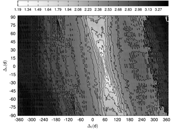
Figure 2: The two-dimensional grid of merit function values for a computer generated random walk and a blend computed from it. The general minimum must indicate the true pair of long and short delay values. The plot demonstrates degeneracy in full-scale computations well – there is obvious symmetry between the areas for positive and negative values of short delays. Values on the colour key represent the $log(D^{2})$ and spacing of the contours. The same type of colour key is used in all two-dimensional plots.

It is also important to check how the actual distribution of time moments in input data sets influences the statistical weights in the final expression for dispersion. Even in the case of the comparison of two pure (one of them shifted) lightcurves, it is not ruled out that for a particular time delay the observations of one curve occur just in the gaps of the other. The well-known controversy on the time delay of the classical double quasar QSO 0957+561 was just a result of this kind of accident (see for details Press et al. 1992a ; 1992b ; and Pelt et al. Pelt94 (1994)). Multidimensional graphs of the parameter dependent sums of weights from Eq. 5 can reveal regions where there is not sufficient information to estimate the parameters of the model.

4 Tests with simulated data sets

Our goal in this paper is to show that the approach described above can be useful – if not generally – then in many interesting situations. We do not have observed data sets for real systems at our disposal that are long enough and have been measured for blended systems. Thus we have to use computer-generated models. We hope that availability of the new method gives an extra motivation for astronomers observing at telescopes with modest resolutions to carry out long monitoring programmes for gravitational lens systems.

The generation of simulated data is simplified by the fact that model curves for different images can be computed from the same source curve. We can apply different shifts to time points of a given or generated sampling scheme, then interpolate values from the source curve at shifted positions, and finally combine the obtained values into blends. To achieve an appropriate degree of realism, we often used time points and weighting sequences from real observations. This allowed us to analyse very irregular and inhomogeneous distributions with caps.

In most cases we used a simple random walk procedure to generate the source variability curves. The time steps for the curves were selected according to two principles: they must be shorter than typical sampling intervals and they must be longer than typical photometric integration times. A random value of $\pm 1.0$ was assigned cumulatively to each step in the intensity scale. If we wanted to model actual observations (especially to use their statistical weight systems), then the resulting curves were appropriately scaled. One of the generated curves and the blend constructed from it is shown in Fig. 3.

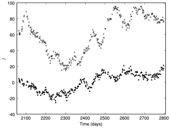
Figure 3: A basic computer-generated random walk $C$ (lower curve) and a computer generated blend curve $A$ ($\Delta_{l}=50.2$, $\Delta_{s}=10.6$, the amplification parameter $\alpha=1.3$; we added $5\%$ noise to both curves and shifted the blend up by $60$ units).

It was interesting to observe that sometimes the generated curve was quite poor in features (minima and maxima, etc.). In these cases we discarded them. There is a similar effect when dealing with actual lens systems. A quasar can be “quiet” for a long time and its photometry is not sufficient for time delay estimation.

4.1 Random sampling

Figure 4: A classical dispersion spectrum computed for the computer generated curve $C$ and the artificial blend $A$. It reveals a shift $\Delta t\approx 59$ days. However, the blend was generated by using a long delay value $50.2$ days and a short delay $10.6$ days. Consequently, blending can mask proper time delay values. The fully resolved case is shown in Fig. 2.

We started our analysis with a simple sampling scheme where the initial time points were generated by using random step sizes from the interval $[0.2,1.8]$ days. The generated time points were then used to read off (using appropriate time shifts and linear interpolation) three different data sequences for the images $C$, $A1$, and $A2$. From the two last images we formed the blend $A=A1+\alpha A2$ with a fixed amplification ratio $\alpha$. In a particular example displayed in Figs. 2 - 4, the following parameters were used: the “long” time delay between $C$ and $A1$ was $\Delta_{l}=50.2$, the “short” delay between the blend components was $\Delta_{s}=10.6$, and the amplification parameter $\alpha=1.3$. To take into account daylight and randomly changing observational conditions, part of the time points were discarded. A typical run of our scheme is given in Fig. 3. From the initially generated $734$ sample points, only $306$ were left in the time series. Finally, we added a random 5% Gaussian noise component to the curves $C$ and $A$.

The two resulting model curves $C$ and $A$ can be used as input for a standard time delay estimation procedure. As seen from Fig. 4, in this example there is a quite well pronounced global minimum in the dispersion curve, but its position is at $\Delta t\approx 59$ days. Blending can move dispersion minima from one place to another.

To recover both delays, we need to apply our new method with artificial blends. First we form a three-parameter search grid $[-360,360:1.0]\times[-90,90:1.0]\times[0.6,1.6:0.1]$ and compute the merit function $D^{2}$ values for each grid point. The value for downweighting parameter $\sigma$ was taken at $2.5$ days. (See Sect. 6 for discussion on choosing the value of parameter $\sigma$.) The parameter combination for the minimum value of the merit function is then selected as the solution. In the current example the best triple occurred at $\Delta_{l}=50$ days, $\Delta_{s}=11$ days, and $\alpha=1.1$. The two-dimensional slice at $\alpha=1.1$ of the search grid is given in Fig. 2. In this plot we can clearly see the degenerate character of our procedure. Depending on the ordering of the blend components, we can attain the deepest minima in two symmetrically placed areas. Formally, both global minima are of equal value, but typically the actual merit function values for both minima differ slightly. If we do not have any additional information (say from deep lens system images) we can just formally select the strongest minimum. Another interesting point of the current example is the fact that our algorithm did not exactly recover the amplification ratio parameter (we found 1.1 instead of 1.3). This is quite typical – for every particular pair of delay values the merit function dependence on the parameter $\alpha$ is quite weak and the corresponding curve has a wide minimum around the correct value.

For high quality data (with small errors) we can look for a final solution with higher precision. For each strong minima found during the rough analysis, we can build refined local parameter grids in the vicinities of the preliminary solutions. An example of such local refinement is given in the next subsection.

4.2 Real sampling

To test our method under real sampling conditions, the time points from the observational data by Schild were used to sample the $C$ and $A$ curves built from a computer-generated random walk pattern. The standard errors given by Schild were scaled according to the ratio of the full amplitudes of the real and simulated data. Next these scaled errors were used as standard deviations for Gaussian noise components, which were added to each point of simulated data. The resulting curves for one particular run are shown in Fig. 5.

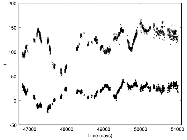
Figure 5: A random walk $C$ (lower curve) and a blend $A$ (upward-shifted curve) with real sampling.

The values of parameters used in this simulation were: $\Delta_{l}=420.15$ days, $\Delta_{s}=20.21$ days, $\alpha=0.8$. We selected a 4202 day time-interval from Schild’s observations and the number of data points in the input table was 1032. A crude search grid $[-150,1000:1.0]\times[-200,200:1.0]\times[0.6,1.6:0.1]$ was used to estimate the amplification parameter $\alpha$. The grid slice with the best value $\alpha=0.9$ was then used to refine other two parameters. (Here and in the next section the value for the downweighting parameter $\sigma$ was taken at $7$ days.) Finally we got the estimates for the delays $\Delta_{l}=420.2$ days, $\Delta_{s}=20.0$ days. The plot of merit function values in the slice $[-150,1000:0.1]\times[-200,200:0.1]$ is shown in Fig. 6. Again, we can see the two symmetrically placed minima.

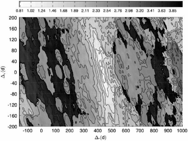
Figure 6: Merit function values for simulated data and real sampling.

To see how observational errors would affect the results, we performed an additional experiment in the vicinity of the obtained solution. We added gradually varying levels of Gaussian noise to the simulated data and evaluated merit function values for the slice $[360,480:0.1]\times[-40,40:0.1]$ ($\alpha=0.9$). The corresponding plots for the four noise levels are given in Fig. 7. It is clearly seen how the minima are smeared out when the noise level rises. From Table 1 we can see how the global solution behaves when noise is added. As was mentioned above, sometimes the solution can jump to its mirror place (and in this case we essentially do not lose it). For higher noise values we can completely lose the correct solution. When planning for a long time photometric monitoring it is reasonable to establish the appropriate levels of measurement precision. For that purpose similar model calculations as carried out in this section can be useful.

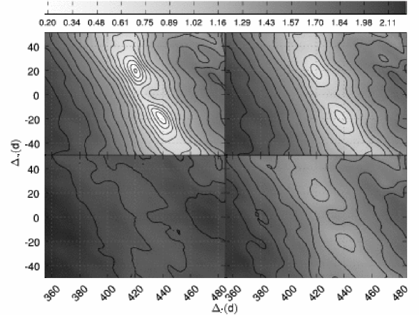
Figure 7: Vanishing of the characteristic minima of the merit function values due to observational errors. The noise levels are (clockwise from upper left): 0%, 2%, 5%, and 10%.

Table 1: Location of global minima depending on added Gaussian noise.

Noise	$\Delta_{l}$	$\Delta_{s}$
(percent)
0	420.6	19.0
1	420.5	19.9
2	419.9	19.1
3	438.5	$-19.0$
4	423.4	20.0
5	419.5	26.9
6	417.5	80.9
10	480.0	46.9
15	499.4	80.9
20	481.4	43.9

4.3 Error estimation

To test statistical properties of the new method we used Monte Carlo type calculations. We added appropriately scaled Gaussian noise components to the noise-free model curves from the previous section, so that the expected signal-to-noise ratios were the same as those for Schild’s data. Using Estonian GRID resources, we repeated this 3500 times and stored the obtained optimal parameter triples. From this resulting table we calculated the average values and standard deviations: $\Delta_{l}=419.6\pm 0.8$ and $\Delta_{s}=20.14\pm 1.22$ days, $\alpha=0.94\pm 0.10$. The resulting biases $419.6-420.15$, $20.14-20.21$ and standard errors for this particular experiment setup are reasonably small.

5 Results for a real system

To evaluate the new method in a more realistic context, we used the master data set for the double quasar QSO 0957+561 A,B kindly provided by Rudy Schild (6806 days, 1233 time points, R-band optical CCD photometry). As far as we know, the components of the system itself cannot be considered as blends and consequently we used this data set as a model for time point spacing and observational error distribution for a long and realistic monitoring programme, as was discussed in Sect. 4.2. In the course of experimentation we also performed some calculations with the full Schild data set and got unexpected results. Assuming that $B$ is a blend, we indeed got a distribution characteristic to the blended case, shown in Fig. 8. The estimates for the time delays in real data are $\Delta_{l}=412,\Delta_{s}=22$ days. The amplification factor was held fixed at $\alpha\equiv 1.0$. ($\alpha\approx 1.0$ is the expected value for short $\Delta_{s}$). In the current section, the value for the downweighting parameter $\sigma$ was taken $10$ days.

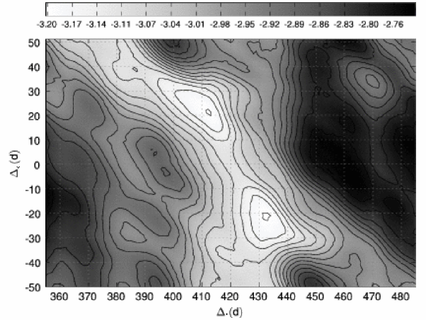
Figure 8: Merit function values for the actual double quasar data. It differs significantly from Fig. 9.

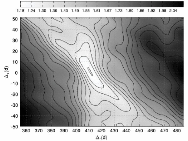
Figure 9: Merit function values for a random walk and its shifted version ($\Delta_{l}=412$ days). Timepoints and standard errors are from Rudy Schild’s monitoring programme.

To convince ourselves that the symmetric minima in Fig. 8 are not caused by boundary effects of our computational algorithm, we performed some additional tests. First we used the real time moments and error estimates from the same data set and built a pair of artificial curves with a given single time delay between the two curves $\Delta_{l}=412$. Then we disturbed both curves by appropriately scaled random errors. The resulting two-dimensional slice of the merit function is shown in Fig. 9. It is well seen that there is one unique global minimum near the true delay value, indicating that we do not have a blend here, the delay applied is recovered and the estimated short shift value (if we assume that the B curve is a blend) is zero. Consequently, our method does not generate symmetrically placed minima just as an artifact of the procedure.

Finally we built an artificial blended model with the long and short delays found from the real curves $A$ and $B$. The resulting grid for the optimal amplification parameter is shown in Fig. 10. From the last simulation we found $\Delta_{l}=412$, $\Delta_{s}=25$ days, indicating that the time delay values found from the real data are real. The three-day long estimation error in short shift characterises the precision of the algorithm at the given level of observational accuracy.

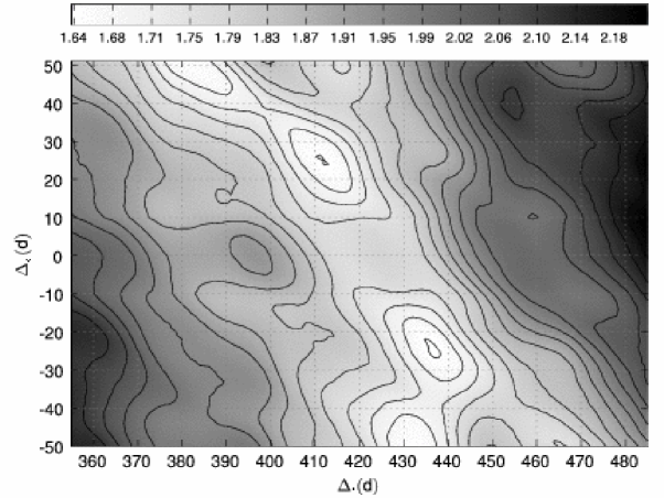
Figure 10: Merit function values for a computer generated random walk and the blend computed from it using the parameters found from the real observational data.

To check how statistically stable the merit function values are for different parameter combinations, we calculated expected sums of weights for the time delay grid of Schild data. As it is seen from Fig. 11, $\Delta_{l}=412$ and $\Delta_{s}=22$ days fall into the region of higher weights and should be considered a reliable result. It is currently very difficult to tell why the $B$ curve of the classical double quasar behaves as a blend. It is known that there is something wrong with the estimated time delays and magnification ratios (if optical data is compared with radio data). The peculiar form of microlensing proposed in Press (Press98 (1998)) can solve the problem of magnification ratios. However, it is hard to expect that the spacing of microlensing events in time can mimic a proper blend. In another development, Goicoechea (Goicoechea (2002)) singles out the different features in the double quasar lightcurves which give different values for time delays. As a possible explanation he uses a quasar model with spatially distant flares, as discussed also in Yonehara (Yonehara01 (1999)) and Yonehara et al. (Yonehara02 (2003)). Similar and even more radical ideas can be found in a recent work by Schild (Schild05 (2005)). Our computations show that not only single events, but the full $B$ curve of the system can be decomposed into a sum of two similar and shifted curves. What theoretical interpretation can be given to this phenomenon remains an open question.

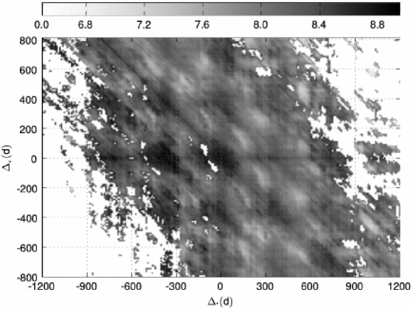
Figure 11: The expected sums of weights for the time delay space of Schild’s data. Zero values represent areas with unphysical negative parameter $a$ values as described in the text.

6 Discussion

Above, we tried to demonstrate that a very interesting data processing method exists, which allows us to estimate integral time-delay systems for blended (not fully resolved) lightcurves. There are not yet enough real observed sequences to evaluate the full potential of the new method, but our computations allow us to get at least a preliminary idea about the applicability of such algorithms. When planning a new monitoring programme we suggest to consider the following aspects:

• The total time base of observations must be determined from the expected length of the longest time delays. We cannot sensibly find longer time delays from the observed time series, than about half of the length of the time series itself.

• Sampling should be dense enough to match the characteristic periods of variability of the source quasar. In more precise terms – the sums of weights for every parameter combination to be compared must be large enough to avoid statistically unstable merit function values.

• Sampling determines the shortest possible delay we are able to find from the particular data. If the downweighting parameter $\sigma$ (see formula 3) is too small for a given sampling, we will have too few pairs in the calculation of the merit function and the map of $D^{2}$ will be poor due to noise and boundary effects. On the other hand, enlargement of $\sigma$ is limited because of the smoothing effect of this parameter – using larger $\sigma$ reduces the possibility of finding shorter time delays. As a rule of thumb $\sigma$ should be kept equal to or smaller than half of smallest possible time delay $\Delta_{s}$ we are trying to find. For sound statistics, we should have on the average at least 3–5 pairs for every observed time point when combining and subtracting the time series. In practice it would be useful to carry on computations with varying values of $\sigma$ to check statistical stability and robustness. See for instance Pelt (Pelt96 (1996)) where such an analysis was used for a simple case of delay estimation.

• A sufficiently dense and truly random distribution of the time points is best for the method described above. The strongest source of uncertainty for the described algorithms is periodicity of data gaps. Unfortunately, ground-based astronomical observations tend to be of this kind. To lessen the effect of gaps, combined observations from different sites can be used.

• As we saw in Sect. 4.2, observational errors for typical experimental setups must be kept under 5% of the amplitude of lightcurve.

• As a sanity check, it is worth to compute merit function values for a larger parameter grid. Then the overall pattern of symmetrically shaped and mirrored minima allow us to get the general impression of the validity of our solutions.

The software modules we have developed can be used to model situations that can occur in real long-time monitoring programmes. By varying model parameters we can estimate sufficient durations for observational sessions and also the accuracy of observation needed. Unfortunately, even accurately planned sessions can result in a failure because the source quasars themselves can show persistent stationarity or the time series observed can be contaminated by strong microlensing. It is not ruled out that the proposed method can be used in absolutely different contexts. One of the applications we are presently considering is disentangling echo components in certain high energy events of cataclysmic stars.

7 Conclusion

A method of finding time delays from photometry of unresolved gravitationally lensed quasar images has been developed and tested using simulated and real data sets. It can be used to analyse already existing data sets and also to plan new observations. We encourage observers to run long time monitoring programmes of blended images to reveal time delays from obtained data.

- (1) Barkana R., 1997, ApJ 489, 21
- (2) Burud I., Magain P., Sohy S., Hjorth J., 2001, A&A 380, 805
- (3) Chartas G., Dai X., Garmire G.P., in Carnegie Observatories Astrophysics Series, Vol.2: Measuring and Modeling the Universe, ed. W.L. Freedman, 2004
- (4) Dai X., Chartas G., Agiol E., Bautz M.W., Garmire G.P., 2003, ApJ 589, 100
- (5) Fassnacht C.D., Pearson T.J., Readhead A.C., et al., 1999, ApJ 527, 498
- (6) Fassnacht C. D., Xanthopoulos E., Koopmans L. V. E., Rusin D., 2002, ApJ 581, 823
- (7) Geiger B., Schneider P., 1996, MNRAS 282, 530
- (8) Gil-Merino R., Goicoechea L. J., Serra-Ricart M., et al., 2001, MNRAS 322, 397
- (9) Gil-Merino R., Wisotzki L., Wambsganss J., 2002, A&A 381, 428
- (10) Goicoechea L.J., 2002, MNRAS 334, 905
- (11) Hjorth P.G., Villemoes L.F., Teuber J., Florentin-Nielsen R., 1992, A&A 255, L20
- (12) Kochanek C. S., Mochejska B., Morgan N. D., Stanek K. Z., 2006, ApJ 637, L73
- (13) Kundić T., Turner E.L., Colley W.N., et al., 1997, ApJ 482, 75
- (14) Morgan N.D., Caldwell J.A.R., Schechter P.L., Dressler A., Egami E., Rix H.-W., 2004, AJ 127, 2617
- (15) Pelt J., Hoff W., Kayser R., Refsdal S., Schramm T., 1994,A&A 286, 775
- (16) Pelt J., Kayser R., Refsdal S., Schramm T., 1996, A&A 305, 97
- (17) Pelt J., Hjorth J., Refsdal S., Schild R., Stabell R., 1998, A&A 337, 681
- (18) Pelt J., 2005, in e-Proceedings of the GLQ Workshop (http://grupos.unican.es/glendama/e-Proc.htm), C5
- (19) Pijpers F.P., 1997, MNRAS 289, 933
- (20) Press W.H., Rybicki G.B., Hewitt J.N., 1992a, ApJ 385, 404
- (21) Press W.H., Rybicki G.B., Hewitt J.N., 1992b, ApJ 385, 416
- (22) Press W.H., Rybicki G.B., 1998, ApJ 507, 108
- (23) Schild R., Thomson D.J., 1997, AJ 113, 130
- (24) Schild R., 2005, AJ 129, 1225
- (25) Yonehara A., 1999, ApJ 519, L31
- (26) Yonehara A., Mineshige S., Takei Y., Chartas G., Turner E.L., 2003, ApJ 594, 107