Six large coronal X-ray flares observed with Chandra

Abstract

Aims. A study of the six largest coronal X-ray flares in the Chandra archive is presented. The flares were observed on II Peg, OU And, Algol, HR 1099, TZ CrB and CC Eri, all with the High Energy Transmission Grating spectrometer (HETG) and the ACIS detectors.

Methods. We reconstruct an Emission Measure Distribution $EMD(T)$, using a spectral line analysis method, for flare and quiescence states separately and compare the two. Subsequently, elemental abundances are obtained from the $EMD$.

Results. We find similar behaviour of the $EMD$ in all flares, namely a large high-$T$ component appears while the low-$T$ ($kT<$ 2 keV) plasma is mostly unaffected, except for a small rise in the low-$T$ Emission Measure. In five of the six flares we detect a First Ionization Potential (FIP) effect in the flare abundances relative to quiescence. This may contradict previous suggestions that flares are the cause of an inverse FIP effect in highly active coronae.

1 Introduction

Table 1: Observations used in this work.

Obs. ID	HD	Other Name	Exposure (ks)	Start Date	Type	Radius	Distance (pc)H	Porb (d)
1451	224085	II Peg	43.3	1999-10-17 23:28:28	K2IV+?	2.2S	42.34	6.7
1892	223460	OU And	96.9	2001-08-11 00:18:00	Single G1IIIe	9F	135
604	19356	Algol	52.4	2000-04-01 02:20:34	B8V+G8IIIB	2.8/3.54B	28.46	2.86B
62538	22468	HR1099	95.9	1999-09-14 22:53:10	G5IV+K1IVS	1.3/3.9S	28.96	2.84
15	146361	TZ CrB	84.8	2000-06-18 13:41:55	F6V+G0VS	1.22/1.21S	21.69	1.14
6132	16157	CC Eri	30.95	2004-10-01 01:46:49	K7Ve/M4S	0.7/?S	11.51	1.56
4513	16157	CC Eri	89.45	2004-10-01 20:54:39	…	…	…	…

H - The HIPPARCOS catalog (Perryman et al., 1997)

S - Strassmeier et al. (1993)

B - Budding et al. (2004)

F - Fekel et al. (1986)

The ongoing multi-wavelength research on stellar coronae has shown that coronal activity in cool stars is closely related to the magnetic activity. While in the solar case the coronal structures are spatially resolved, one has to rely on accurate spectroscopy in analyzing the unresolved stellar corona. Although showing general similarity to the sun, some stellar systems exhibit coronal activity 3-4 orders of magnitude more energetic than in the sun, especially during large flares. Whether this indicates a scaled up version of the solar coronal activity or a differently structured corona is not yet clear.

Another effect which is not well understood is the abundance variations between the photospheres and coronae of the stars. In the solar case this has been known as the First Ionization Potential (FIP) effect (Feldman, 1992), where compared to their photospheric abundances, elements with low FIP (under$\sim$10 eV) are over-abundant relative to elements with higher FIP. Many systems show this effect, but some active systems show an opposite effect where it is the high FIP elements who are over abundant. This was labeled the Inverse FIP (IFIP) effect (Brinkman et al., 2001). Audard et al. (2003) found that highly active RS CVn binaries show an IFIP effect while less active systems show either no effect or a solar FIP effect. Telleschi et al. (2005) found a related result in a sample of solar like stars, where abundances change from IFIP to FIP with the age (and decreasing activity) of the star. This has led to the suggestion that activity affects coronal abundances, possibly by flares that evaporate high-FIP material from the lower chromosphere to the corona (Brinkman et al., 2001) and by electric currents that suppress the diffusion of low-FIP species to the corona (Telleschi et al., 2005). Observationally, however, the association to date of flares with FIP or IFIP effects is ambiguous. Güdel et al. (1999) and Audard et al. (2001) found an increase in low FIP abundances during flares on the RSCVn UX Ari and HR 1099, respectively. In some cases the variations in abundances were not FIP-related (Osten et al., 2003; Güdel et al., 2004). In other cases, no abundance variations were found at all, e.g., Maggio et al. (2000) and Franciosini et al. (2001), though the last two works are based on low spectral resolution data.

The X-ray band offers several advantages in the study of stellar flares. The high temperatures in the flares, typically with $kT\leavevmode\nobreak\ \geq 1$ keV, mean that most of the emission is in the X-ray band and the major emission lines of the highly ionized elements fall in the 1.8 to 40 Å range. This provides measurements of line fluxes from up to 10 Fe K- and L- shell ionization degrees (Fe XVII to Fe XXVI), as well as from the two K-shell ions of the other common elements. While previous instruments limited plasma emission models to two- or three- thermal components, line resolved spectra from Chandra enable the reconstruction of a more accurate distribution of plasma temperatures, as well as better measurements of electron densities and abundances.

The reconstruction of the emission measure distribution ($EMD$) that describes the plasma thermal structure, and the measurements of abundances are difficult, not only because the two are entangled, but also due to the poor mathematical definition of the problem as shown by Craig & Brown (1976). Small variations of observed line fluxes result in large variations in the derived $EMD$. Almost any variation of the $EMD$ can be accommodated to produce the same spectra, up to measurements uncertainties, if done on small enough temperature scales. Consequently, many authors avoid setting confidence intervals on their fitted $EMD$, or use $EMD$ smoothing, which makes the comparison of $EMD$s produced by different methods a difficult task. The correlation between $EMD$ parameters and deduced abundances is often neglected or ignored.

In this work, we scanned the public Chandra archive for bright flares that enable good line flux measurements. Six such flares were found on the systems: II Peg, OU And, Algol, HR 1099, TZ CrB & CC Eri. While these are not the only flares in the archive, they represent the brightest and best resolved flares available. Some of these observations have been analyzed before, but not always with regard to the flare and not in a way that allows a comparison with other analysis methods. We refer to these previous works in section 5.2.

We apply the same analysis methods, employing the derivation of a continuous EMD and relative abundances, for the six targets in flaring and quiescence states. The method is based on the one used in Nordon et al. (2006). Emphasis is given to the ability to compare the results in a statistically significant way in order to seek real variations in the thermal structure and abundances between flare and quiescent states. In particular, we want to establish whether the large flares had a statistically significant effect on the coronal abundances and whether it is FIP-related.

2 Observations

2.1 The Sample

The Chandra public archive was searched for observations of cool stars (spectral types A to M) in any system configuration, featuring strong, long-duration flares. The main selection criterion was the requirement for enough photons in the flare to allow a detailed spectral analysis. So, while there are other observed flares not included in this work, this sample represents the best flares, in terms of photon counts, observed with Chandra. All grating observations were examined, however, the selected sample happens to contain only the ACIS+HETG instrument configuration, which is the most common configuration used for coronal targets.

The details of the selected observations and targets are summarized in table 1. The data for CC Eri are composed of two observations separated by a short time gap. The flare occurred at the end of the first observation and the last part of the flare decay was cut-off. Due to low flux in the quiescence state, we integrated both the period before the flare from the first observation, and the entire second observation for the spectral extraction of the quiescence state.

2.2 Light Curves and Spectra

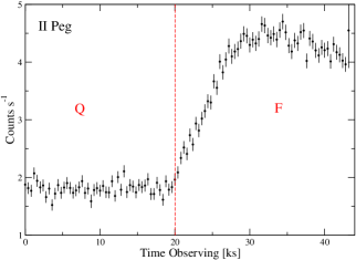
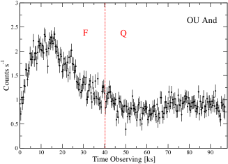
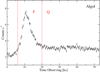
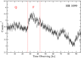
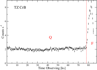
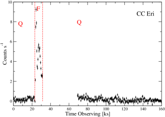
Figure 1: Light curves of the observations using 400 s bins. All orders of diffraction are included and background is subtracted. The vertical dashed lines indicate the segments considered as flaring or quiescence and marked with letters F and Q respectively. The CC Eri observation consists of two nearly continuous observations.

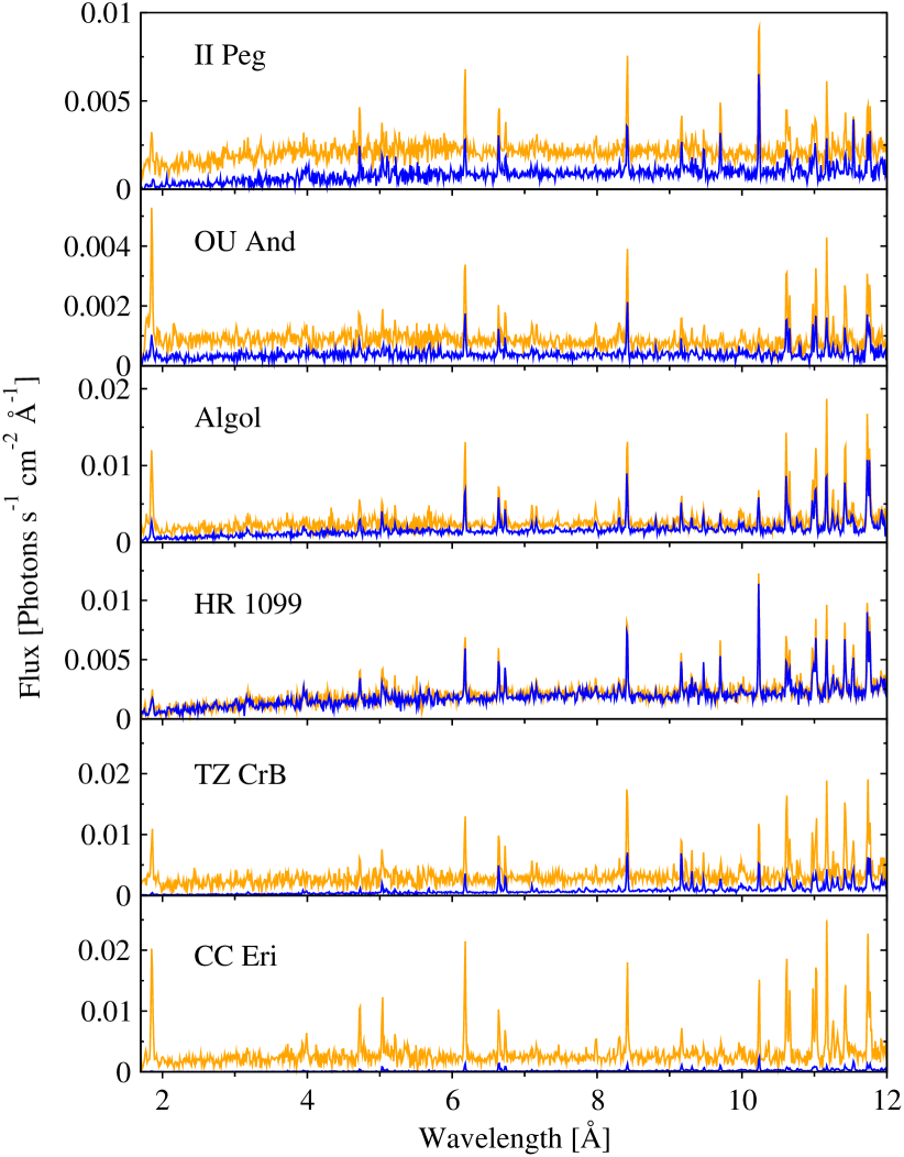
Figure 2: Time averaged flare and quiescence spectra of the 6 targets in the 1.7-12 Å range. HEG and MEG gratings 1st orders are combined at MEG resolution and 0.01 Å bins. Orange is flare and blue is quiescence.

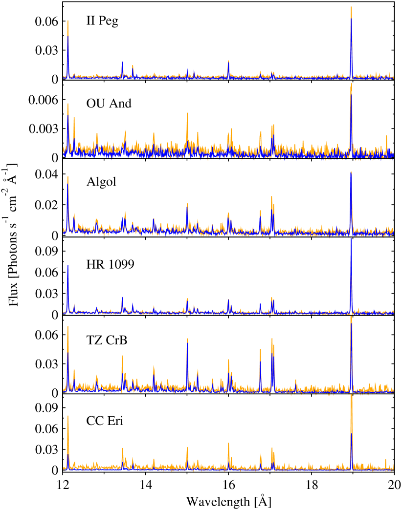
Figure 3: Time averaged flare and quiescence spectra of the 6 targets in the 12-20 Å range. HEG and MEG gratings 1st orders are combined at MEG resolution and 0.01 Å bins. Orange is flare and blue is quiescence.

Light curves were produced using combined counts of the High (HEG) and Medium (MEG) energy grating arms of all orders as well as the zero-order region. Background, though negligible, was estimated and subtracted using off-source CCD regions. The light curves are presented in Figure 1 using 400 s bins. Segments used for flare and quiescence spectra extraction are marked with F and Q respectively.

Flare and quiescent spectra are presented in figures 2–3 and correspond to the time segments of the observations marked in figure 1. In the Algol observation, the time segment before the flare was excluded as the system was still in eclipse. The plots are in 0.01 Å bins and use combined fluxed spectra of HEG and MEG.

3 Modelling Method

3.1 Emission measure distribution

While seeking the plasma parameters that reproduce the properly measured fluxes of several selected lines, we are particularly interested in examining the thermal structure and elemental abundances independently. Therefore, we develop and use a method that disentangles the mutual dependence in a simple way. The continuum emission is problematic for two reasons; One being the typical low level of continuum emission in quiescent states. The other reason is the lack of unique features in the continuum, which makes the distinction between thermal and non-thermal components, or between high-$T$ components and low metalicity, difficult and ambiguous. Better constraints are provided by the high energy end of the bremsstrahlung spectrum, but in cases of a wide temperature distribution even the distinctive bremsstrahlung peak may be blurred. Moreover, in flares, the continuum turnover is often beyond the instrument band. Thus, we avoid using the continuum and rely on the more accurate line fluxes.

The observed line flux $F^{q}_{ji}$ of ion $q$ due to the atomic transition $j\rightarrow i$ can be expressed by means of the element abundance with respect to hydrogen $A_{z}$, the distance to the object $d$, the line power $P^{q}_{ji}$, the ion fractional abundance $f_{q}$ and the $EMD$ as:

$$F^{q}_{ji}=\frac{A_{z}}{4\pi d^{2}}\int_{0}^{\infty}{P^{q}_{ji}(T)f_{q}(T)EMD(T)\mathrm{d}T}$$ (1)

The line emissivity $\epsilon^{q}_{ji}(T)=P^{q}_{ji}(T)f_{q}(T)$ describes ion and line specific parameters, while the general plasma parameters are described by the $EMD$ as:

$$EMD=n_{e}n_{H}dV/dT$$ (2)

Where $n_{e}$ and $n_{H}$ are the electron and hydrogen number densities averaged over the volume of plasma in the temperature interval [$T$, $T+\mathrm{d}T$].

The strongest unblended line from each ion is selected for the analysis and density sensitive lines are avoided. Nonetheless, a complete set of ionic spectra are used to account for residual blending. The temperature dependence of the line emissivity $\epsilon^{q}_{ji}(T)$ comes mainly from $f_{q}(T)$ and therefore a second line from the same ion contributes little additional information, except for more photon statistics. It could however, in some cases, provide statistical compensation for uncertainties in the atomic parameters of the strong line.

We use the primary line from every Fe ion (Fe XVII to Fe XXV) in the observed spectra to get a set of integral equations, whose solution yields the $EMD$ scaled by the unknown Fe abundance:

$$F^{q}_{ji}=\frac{A_{Fe}}{4\pi d^{2}}\int_{T_{0}}^{T_{max}}{P^{q}_{ji}(T)f_{q}(T)EMD(T)\mathrm{d}T}$$ (3)

In order to include lines of other elements, but without the need to fit their abundances, we use ratios of the He-like to H-like line fluxes, from the same element. Thus, the element abundance $A_{z}$ cancels out. This adds another set of equations that constrain the shape of the $EMD$, but do not depend on the abundances:

$$R_{z}=\frac{F^{He-like}_{ji}}{F^{H-like}_{lk}}=\frac{\int_{T_{0}}^{T_{max}}{P^{He}_{ji}(T)f_{He}(T)EMD(T)\mathrm{d}T}}{\int_{T_{0}}^{T_{max}}{P^{H}_{lk}(T)f_{H}(T)EMD(T)\mathrm{d}T}}$$ (4)

The X-ray spectra we use here include as many as ten Fe ions, but no more than two ions from other elements. For every observation we are able to use similar equations, but different specific ions, depending on which lines have a sufficiently good signal.

The line fluxes and flux ratios are then fitted using the least squares best fit method to solve this set of equations for the $EMD$, where the $EMD$ is expressed by a parameteric non-negative function of $T$ (see details in section 3.3). The minimization algorithms used are Levenberg-Marquardt and Nedler-Mead (simplex) alternately and combined, taking the best result. The fit yields the estimated shape of the $EMD$, independent of any assumptions for the abundances, and is scaled by the Fe abundance. In other words, we solve for the product of $A_{Fe}\cdot EMD$. The integration in eqs. (3, 4) is started at $kT_{0}=0.2$ keV and cut-off at $kT_{max}=10$ keV, under and over which the $EMD$ is completely degenerate, as no new lines emerge from these temperature regimes. This means that some of the flux in high-$T$ lines may originate from plasma at even higher temperatures, the effect of which will be emission measure (EM) added to the last high-$T$ bin. The same applies to the lower temperature cut-off. Some emission in the low-$T$ lines may originate from temperatures lower than the cut-off. For this reason, we avoid using lines with significant emissivity below the cut-off temperature, even if they are available (e.g. O VII). The coolest forming ion we use is O VIII whose emissivity peaks at $\sim$0.25 keV and for which over 95% of the emissivity lies above the threshold. Gu et al. (2006) showed that below 0.2 keV HETG cannot constrain the $EMD$. The abundance-independent approach, namely using abundance independent equations for fitting the $EMD$ and then using the $EMD$ to resolve the abundances, has been used in other works as well, for example: Schmitt & Ness (2004) and Telleschi et al. (2005).

The atomic data for the line powers are calculated using the HULLAC code (Bar-Shalom et al., 2001). The ionic abundances ($f_{q}$) for: Fe, Ar, S, Si, Mg are taken from Gu (2003). Mazzotta et al. (1998) is used for the other elements.

3.2 Line fluxes

In order to measure the line fluxes and solve for possible line blending, we preform an ion-by-ion fitting to the spectra. The line powers for each ion are calculated at its maximum emissivity temperature and then passed through the instrument response. This accounts for all of the lines and fixes the ratios of lines from a given ion.

The observed spectrum is then fitted by sets of complete individual-ion spectra simultaneously, together with a bremsstrahlung continuum, composed of several discrete-temperature components. This results in an excellent fit that accounts for all the observed lines and blends. Since we ultimately use only several selected lines for the analysis, we make sure that they fit well and the fitting of the other lines serves for estimating the blends in the selected lines (which is small to begin with). The fitted continuum parameters are independent of the reconstructed $EMD$ and are not used in the following analysis. The synthetic continuum serves only for measuring line fluxes above it. Due to the high resolving power of the HETG that produces narrow line profiles and the ionic spectra that include all lines that may contribute to a pseudo continuum, the local continuum level is reliable. The narrow line profiles of HETG also mean that slight deviations in local continuum level have little effect on the measured line flux. This process is similar in principle to the one used in Behar, et al. (2001) and in Brinkman et al. (2001).

The line fluxes measured from all the observations and used in the following analysis are listed in tables 4-6 in the appendix.

3.3 EMD parametrization and fitting

Our goal is to compare the $EMD$ of the flare and quiescence states. It is important to note that the solution for the $EMD$ is not unique as is the case with integral equations of this sort (Craig & Brown, 1976). On scales much smaller than the width of the ions emissivity curves, or in temperature regions where the relative emissivities vary slowly, there is no way of constraining the shape of the $EMD$ from measurements alone. However, in order to be able to compare different $EMD$ solutions, we need to have meaningful confidence intervals. Currently, we do not have a theoretical model that describes the $EMD$ of a full corona, although ther are theoretical predictions for the $EMD$, under various assumptions. We therefore make no assumptions as to the shape of the $EMD$ and choose to fit a staircase shaped function to allow for local confidence intervals estimates. It also makes the equations for the Fe line fluxes, which give the best constraints, linear in the fitted parameters.

$$EMD(T)=\{C_{n}\hskip 10.0ptT_{n}<T<T_{n+1}\>;\>n=0...N-1\}$$ (5)

Where $N$ is the number of EM temperature bins, $T_{n}$ is the lower temperature of bin $n$. $C_{n}\geq 0$ is the parameter to be fitted, which is the averaged $EMD$ over the bin. The confidence intervals are calculated using the inverse $\chi^{2}$ distribution, meaning we search the parameter space for the $\chi^{2}$ contour that gives a deviation from the best-fit that corresponds to the requested confidence level. A $1\sigma$ deviation is defined as the contour of $\chi^{2}_{min}+1$. The selection of the number of bins and their widths is not trivial and optimal $EMD$ binning can vary between different spectra. The line emissivity curves have considerable widths and some extend to temperatures much higher than their peak emissivity, resulting in strong negative correlations between the $EMD$ in neigbouring bins. Since, as discussed above, we are interested in meaningful confidence intervals, we cannot use many narrow bins, as this will result in excessive error bars. By making narrow bins they also become closer in temperature, the emission contribution of neighbouring bins becomes similar, thus increasing the degeneracy. Ultimately, if meaningful confidence intervals are to be obtained, the number of bins has to be kept small, and the tradeoff between temperature resolution (number of bins) and constraints (degeneracy of the solution), optimized. No smoothing algorithm is applied to the $EMD$.

In addition, we fit an $EMD$ parameterized as an exponent of a polynomial ensuring that the $EMD$ remains positive:

$$EMD(T)=\exp\left(\sum_{n=0}^{N}{C_{n}P_{n}(T)}\right)$$ (6)

where $P_{n}(T)$ is an $n$-degree polynomial represented as a Chebyshev polynomial for numerical convenience and summed up to $N=7$. This is similar in principle to the method used by Huenemoerder et al. (2001), but with no smoothing. In this method, local confidence intervals can not be produced, but we use it to verify that our results do not depend on the $EMD$ parameterization.

3.4 Integrated EM

The physical measurable quantity is the observed line flux, which results from the entire plasma (an integration over the $EMD$, eq. 1). Therefore, the meaningful quantity is the integral of the $EMD$ over a range of temperatures. In other words, the total EM in that range. Since emissivity curves are smooth, uncertainties in the exact way the EM is distributed over a temperature range, narrower than the emissivity widths, will not have a significant effect on the total EM in that range. When integrating and taking correlations into account, uncertainties caused by the strong correlation between neighboring $EMD$ bins that were integrated over, disappear. This results in much smaller errors.

Temperature regions with little emissivity variations lead to poor localization of the $EMD$ that in turn create spikes in the fitted $EMD$ if no smoothing algorithm is used. Such spikes in the solution are likely to appear when too narrow bins are used. This reflects the fundamental mathematical instability of the solution. The progressively Integrated EM as a function of temperature (IEM($T$)) provides natural smoothing to these spikes as the confidence intervals always vary smoothly. When comparing two different $EMD$s (e.g., flare and quiescence states), since we propagate the confidence intervals, the IEM indicates with greater certainty where the two solutions differ. It also allows the comparison of results obtained by different methods or by different binning as it clears out correlation related uncertainties. Over-binning, thus, which can make the $EMD$ meaningless, will not render the IEM unusable.

For the staircase $EMD$, the IEM is tracked at each stage of the search for the parameters confidence intervals. This way, we get good estimates for the upper and lower limits of the IEM curve, inside a $\chi^{2}$ surface that represents a $1\sigma$ deviation. We also integrate over the $EMD$ from the exponential model to verify that the IEM is consistent regardless of the chosen $EMD$ parameterization.

3.5 Abundances

In order to extract the X/Fe abundance ratios, we calculate the non-Fe line fluxes predicted by the fitted, Fe-scaled, $EMD$.

$$F^{q}_{ji}=\frac{A_{Fe}}{4\pi d^{2}}\left(\frac{A_{Z}}{A_{Fe}}\right)\int_{T_{0}}^{T_{max}}{P^{q}_{ji}(T)f_{q}(T)EMD(T)\mathrm{d}T}$$ (7)

The ratio of the actual measured fluxes to these calculated fluxes gives the X/Fe abundance values. Note that for calculating abundances, one line from each element is sufficient, while for the $EMD$ equations we require two lines of different ionization degrees. This is why we can estimate abundances for elements not used in the $EMD$ fitting. Such is the case with Oxygen where we exclude O VII as it forms mostly at temperatures below our low-T cutt-off, but use O VIII for the abundace.

Abundance uncertainties are directly related to the specific element line flux errors, but they are also indirectly a result of $EMD$ uncertainties. We take into account the latter by tracking the upper and lower limits on the abundances as we fit the $EMD$ and calculate its confidence intervals. This gives the possible abundance values within a one $\sigma$ variation of the $EMD$. Since $EMD$ is determined mostly by Fe and a combination of other elements, it is justified to treat the two error contributions as uncorrelated. We have also calculated the abundances using the exponential $EMD$ model and verify that the results of the two models are in good agreement.

We do not calculate the absolute abundances, i.e., the abundances relative to hydrogen. The absolute abundaces are sensitive to the continuum, which is produced mainly by the less constrained high-T $EMD$. This is demonstrated in the work of Gu et al. (2006) where different instruments observing the same source produce different absolute abundances, but similar relative abundances. Since we are interested in abundance variations during the flare, we use the relative (to Fe) abundances, obtained strictly from line fluxes.

4 Results

4.1 EMD and integrated EM

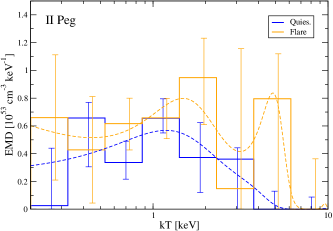
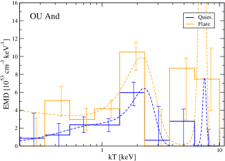
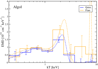
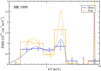
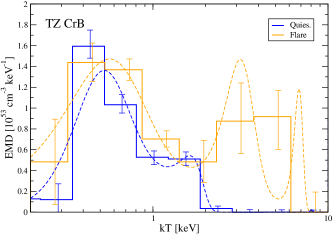
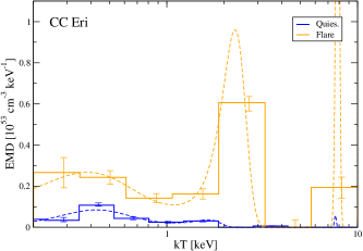
Figure 4: Emission measure distributions for flare and quiescence states. Solid lines are the binned $EMD$ models with 1$\sigma$ errors. Dotted lines are the exponent of polynomials $EMD$ models. For scaling purposes only, a solar Fe/H abundance of 3.24$\times 10^{-5}$ is assumed (Feldman, 1992).

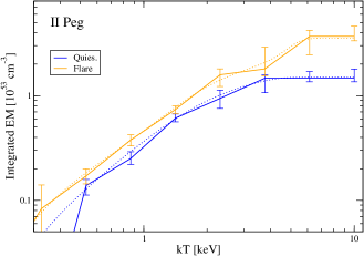
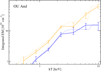
Figure 5: The total EM integrated over the $EMD$ from 0.2 keV to $kT$. Solid line is from the staircase $EMD$ model and includes 1$\sigma$ errors. Dotted line is using the exponent of polynomials $EMD$ model.

The best-fit $EMD$ for each of the six targets is plotted in figure 4. The error bars on the staircase $EMD$ model (eq. (5)) are 1 $\sigma$ errors and include correlation uncertainties. The smooth dashed line with no confidence intervals is the exponential model (eq. (6)). Since the $EMD$ is scaled by the Fe abundance and since we do not measure the absolute Fe/H abundance, we assume in Fig. 4 a solar abundance of 3.24$\times$10^-5 (Feldman, 1992). This has no effect on the following results and is done purely for the purpose of setting a reasonable absolute $EMD$ scale.

In all cases, the two models (staircase and exponential) agree with each other quite well within the errors over most of the temperature range considered. The exponential model tends to place a very sharp peak at $\sim$8 keV, especially for the flaring states. The reason for this is that the constraints on the $EMD$ in this region are almost exclusively set by Fe XXIV and Fe XXV. In order to set the observed line flux ratio only one temperature is needed and the solution tends to a delta function around that temperature. When we look at the staircase $EMD$ we can see from the large correlation-induced error bars in the last bins, that this component can easily be placed in the neighbouring bin without changing the resulting spectrum significantly.

Comparing the flare and quiescence $EMD$ for each target we see a general pattern: At temperatures typical of the quiescence state the $EMD$ is similar or increased by some small factor and at higher temperatures a new component appears during the flare. In CC Eri, the lower-$T$ $EMD$ is increased by a considerable factor of roughly 3. The HR 1099 flare differs from the others by having very little added $EMD$ at temperatures higher than those of the quiescence state.

The integrated EM from zero to $kT$ is plotted in figure 5 for all targets with 1$\sigma$ error bars. The smooth dashed line without confidence intervals is the integral over the exponential model. In the 0.5-2 keV temperature region, where many L-shell emissivity curves peak, the IEM from both models (staircase and exponential) agree very well. At higher temperatures, the localization of the EM is not as good and the two models diverge slightly, but they always do re-converge at higher temperatures, once the integration covers the full range. At 10 keV the total EM is remarkably similar for both models and well within the error bars.

In most of the flares (II Peg, OU And, Algol and TZ Crb) the IEM of the flare, runs parallel to the IEM of quiescence up to $\sim$2 keV in the log-log plot, which indicates that the thermal structure remains the same or uniformly increased by a small factor. In the CC Eri flare, the increase in low-$T$ EM is much more significant and reaches a factor of 4.3 at 2 keV, where the flare IEM is still increasing while the quiescence IEM has nearly reached its maximum value. The HR 1099 flare IEM is generally parallel and above the quiescence IEM, except around 1.5 keV where they are similar.

Several theoretical works attempt to predict the $EMD$ of a static loop or flaring loops. They commonly predict a power law type distribution up to a peak temperature:

$$EMD(T)\propto T^{\alpha-1}$$ (8)

where $\alpha$ is determined by the details of the cooling processes. Note the different definitions of the EMD in various papers. For purely radiative cooling, $\alpha=-\gamma+1$ where $\gamma$ is a parameter (in the range $\gamma\approx 0\pm$0.5) of the approximated radiative cooling function:

$$\Lambda(T)\propto T^{\gamma}$$ (9)

i.e. $\alpha=0.5-1.5$, while for conductive cooling $\alpha\approx 1.5$ and for evaporation $\alpha\approx 0.5$ (Antiochos, 1980). Of special relevance to this work, where we integrate the spectra over the entire flare, is the calculation by Mewe et al. (1997). They predict for a time-averaged $EMD$ of a quasi-statically cooling flaring loop $\alpha=19/8$. Since we can resolve the $EMD$ only down to 0.2 keV, fitting a power law up to the first peak is possible only to in those systems that peak is around 2 keV. We also fitted the flare in the range of 4-10 keV, where the quiescence emission is low. The fits were preformed on the IEM curves as the errors there are smaller. The results are shown in table 2. We see that $\alpha$ is in the range of 1.5-2, which is slightly higher than expected from radiative and conductive $EMD$ models, significantly higher than expected from evaporation models and significantly lower than expected from the effect of time averaging over a single temperature cooling loop.

Table 2: Fitted powerlaws for the EMD.

	quiescence (0.2-2 keV)			Flare (0.2-2 keV)			Flare (4-10 keV)
System	$\alpha$	$\sigma$	red. $\chi^{2}$	$\alpha$	$\sigma$	red. $\chi^{2}$	$\alpha$	$\sigma$	red. $\chi^{2}$
II Peg	1.47	0.14	1.33	1.48	0.18	0.06	0.8a	0.4	0.26
OU And	1.96	0.24	0.51	1.87	0.16	1.4	1.5	0.3	0.2
Algol	1.57	0.07	4.0	1.66	0.11	3.9	0.8	0.2	0.25

^a - Due to low EM at very high T, a temperature range of 2.5-6 keV was used.

4.2 Abundances

The abundances relative to Fe, as calculated from the staircase model are summarized in Tables 7-12 in the appendix. Quoted errors include both flux and $EMD$ uncertainties as explained in section 3.5. Abundances measured using the exponential $EMD$ agree well with these results within a few percent of a std-dev. The difference between the $EMD$ representations is so small that we only quote the values from the staircase model. Since we obtain the element abundance for individual ions, elements with more than one ion in the spectrum may have several abundance values. The abundance value in the table is the statistically weighted average of these individual-ion abundances. Note that abundances derived from different ions of the same element are expected to be consistent, since this was assumed in the $EMD$ reconstruction algorithm (see eq. (4)).

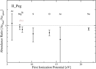
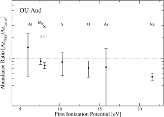
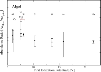
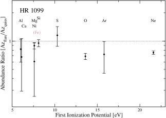
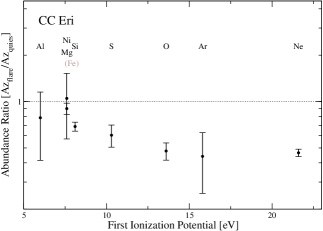
Figure 6: Flare abundances relative to quiescence abundances as a function of FIP.

5 Discussion

5.1 Present work

The $EMD$ plots depict the average variation in the thermal structure of the plasma coupled with possible density variations. The $EMD$ in each temperature bin represents the averaged $EMD$ over the bin temperature range. It is apparent that the systems that are considered coronally active, namely Algol, HR1099 and OU And show a similar $EMD$ shape during quiescence: A gradual increase with $kT$ up to about 2 keV and a sharp drop beyond that, becoming negligible at 3-4 keV. This is in contrast with the two other systems: TZ CrB and CC Eri, which have most of the emission localized around 0.5 keV during quiescence, but still have a small amount of EM up to 2 keV. II Peg is a middle case where the $EMD$ peaks around 1 keV and a significant portion of the EM is likely to be above 2 keV.

Looking at figure 5, for most targets, the flare and quiescence IEM curves run nearly parallel (in log scale) to each other up to a point where the EM in the flare increases sharply relative to quiescence. It is clear that most of the excess EM is located at the very high temperatures, typically above 2 keV. HR 1099 is the exception to this rule as no significant amount of EM is added at high temperatures during the flare. The IEM in CC Eri is unique. There is much excess low-$T$ EM ($\sim$ factor 4) in the flare, starting apparently from the lowest temperatures observed.

The similarity in flare and quiescence $EMD$ at temperatures below 2 keV, differing only by a constant factor was also observed by Nordon et al. (2006) in a flare on $\sigma$ Geminorum. This effect was clear from a direct comparison of the flare and quiescence spectra. In that case, the line emission at wavelengths above 12 Å was increased by a uniform 25%, corresponding to a uniform $EMD$ increase by the same factor under $\sim$2 keV temperature. Audard et al. (2001) also reported a similar effect in a flare on HR 1099 detected by XMM-Newton.

The added EM at low temperatures can be either a real variation of the quiescence corona, or an effect caused by the time averaging of the flare heating and/or cooling. In other words, a narrow temperature component from the flare (moving up or down in $kT$) will mimic a continuous distribution when averaged over time. Ideally, we would repeat the $EMD$ analysis for shorter segments of time to reproduce the time evolution. Unfortunately, that also means higher statistical uncertainties on the line fluxes, leading to too high uncertainties on the $EMD$ to make the comparison feasible. We did extract light curves for the brightest lines in the spectrum and looked for a direct indication of heating or cooling. No clear conclusion could be made. In the case of a narrow temperature component, the cooling through the low-$T$ range would have to be fast enough in order to pass the significant amount of excess EM from high-T to below the minimum temperature, without adding much to the time averaged $EMD$. The fact that this added cool EM is present even in the II Peg observation, where most of the decay phase is not observed, suggests that it is not a time averaging effect, but rather a genuine increase in EM over a broad temperature range in all flares. A note should be added that the $EMD$ is scaled by the unknown Fe abundance relative to H. Therefore, a possible increase in Fe abundance could explain the uniform increase in the cool range $EMD$. This possibility has no effect on, and is consistent with, the FIP related abundance variations which we discuss below.

The contrast between the small low-T EM excess and the large high-T EM excess could be due to rapid expansion (e.g., evaporation, relaxed pinch, loss of magnetic confinement), which results in a rapid loss of high-T EM. In this case, the flare either reaches low temperatures when its EM is small, or the flare originates in a hot environment and therefore cools down only to the (high) ambient temperature.

Table 3: Total integrated EM^a from 0.2 to 10 keV and averaged luminosities^b in the 1.8–20 Å range.

	Quiescence		Flare		EM Ratio	Flare Int.	Total Net Flare
	EM	LX c	EM	LX c	Flare/Quies.	Time	Energy
Traget	[1053 cm-3]	[1030 erg s-1]	[1053 cm-3]	[1030 erg s-1]		[ks]	[1034 erg]
II Pegd	1.47${}^{+0.32}_{-0.11}$	9.8$\pm$0.2	3.7${}^{+0.9}_{-0.35}$	22.5$\pm$0.2	2.5	22.7	28.7$\pm$0.6
OU And	15.25${}^{+4.1}_{-5.0}$	40.6$\pm$0.8	63.2${}^{+8.9}_{-9.4}$	95.5$\pm$1.3	4.1	39.5	216$\pm$6
Algol	3.14${}^{+0.37}_{-0.43}$	7.69$\pm$0.06	8.3${}^{+1.2}_{-1.1}$	12.8$\pm$0.2	2.6	13.7	7.0$\pm$0.2
HR 1099	2.4${}^{+0.5}_{-0.3}$	9.61$\pm$0.08	3.0${}^{+0.5}_{-0.5}$	10.7$\pm$0.1	1.25	15.9	1.85$\pm$0.2
TZ CrB	1.19${}^{+0.07}_{-0.03}$	2.92$\pm$0.02	5.1${}^{+0.7}_{-0.6}$	9.5$\pm$0.2	4.3	6.2	4.1$\pm$0.1
CC Eri	0.079${}^{+0.005}_{-0.007}$	0.223$\pm$0.003	2.0${}^{+0.2}_{-0.2}$	2.42$\pm$0.04	25.3	8.0	1.76$\pm$0.03

^a Using the staircase EMD

^b Luminosities are averaged over the time intervals as indicated on the light curves

^c Luminosity of the averaged spectra during quies./flare states

^d Observation ended while excess flux was still high.

Table 3 summarizes the values of the total integrated EM (last data point in figure 5). We see that in most cases the flares cause an increase in EM by a factor of 2–4. In HR 1099, interestingly, it increased by only 25%, while in CC Eri it increased by a factor of $\sim$25, although the total EM of CC Eri is still very small relative to the other systems. This means that the quiescent corona of CC Eri is very small and the emission in the flare could be attributed entirely to the flare heated plasma. In the other systems we observe a mix of flare plasma with a background of the strong quiescent corona.

Overall, there are no dramatic variations in abundances, but several elements do show a tendency of decreased abundances relative to Fe during the flares, mainly O and Ne. A similar effect has also been observed in a flare on $\sigma$ Gem (Nordon et al., 2006). It should be noted that in those flares where the low-$T$ EM ($kT<$ 2 keV) during the flare is not significantly larger than in quiescence, the measured flare abundances are practically a weighted average of the abundances in the flaring plasma and the background quiescence plasma.

Figure 6 shows the flare to quiescence abundance ratios plotted as a function of FIP. Since the abundances are plotted relative to Fe it means that if the Fe/H abundance has changed in the flare, all the ratios in the figure will be multiplied by a uniform factor of $Fe_{quies}/Fe_{flare}$. This may re-scale the plot, but will not change the pattern or our conclusions. We see that in all flares, with the exception of TZ CrB, high FIP elements show reduced abundances. For the low FIP elements the picture is not as clear as the elements with FIP lower than Fe: Al and Ca, have large error bars. Still, elements with FIP of 8 eV and below seem to vary together with Fe (flare/quies is $\sim$1). This behaviour is similar to the solar FIP effect. TZ CrB is the exception, with no apparent abundance effects as all abundance ratios are consistent with unity.

This is somewhat surprising as other works have shown that increased coronal activity leads to the IFIP effect. Audard et al. (2003) have examined abundances on RS CVn systems and found that high FIP elements were increasingly over-abundant as the typical temperature (used as an indication of activity) increased. Telleschi et al. (2005) have found a similar effect in solar like stars where the FIP effect switched to IFIP as activity increased. For stars with an IFIP corona, chromospheric composition would appear to be FIP in comparison. The change in abundances during the flare indicates that the excess plasma is not heated coronal plasma, but more likely heated chromospheric plasma. This would mean that, if flares are at all responsible for the IFIP effect, the selective element transport would have to operate during the cooling or post-flare stage since we detect a low-FIP enriched composition during the flare itself.

From looking at the light curves in figure 1, we clearly see two types of flare behaviours: Symmetric flares with a sharp peak and a rapid decay (CC Eri & Tz CrB), and asymmetric flares that rise fast, but decay slowly, which creates a broad peak (II Peg, HR1099, OU And). Algol, at first glance, appears to belong to the first kind, but the flare occurred just as the system was coming out of eclipse. As noted by Chung et el. (2004), it is likely that if most of the emission originates from near chromospheric level, the rise phase in the X-ray light curve is governed by the exposure of the flaring region behind the eclipsing companion and not by the rise of the flare. Both of the rapid decay flares occurred on the cooler dwarf stars, while the long duration flares are all on the giant or sub-giant stars. However, CC Eri flare shows the clearest FIP effect in the flare relative to quiescence, similar to the long duration flares, while TZ CrB shows no abundance variations. The sample is too small to draw any substantiated conclusions, but it seems that there is no clear correlation between the type of flare and abundance effects.

5.2 Comparison With Previous Works

Several of the observations used in this work (table 1) were published before by other researchers, although for the most part the focus was not on the flare effects. Also, the methods were different than ours and the presentation of results makes comparisons difficult. We bring here a short summary of the results of those individual works as well as references to other relevant high-resolution X-ray observations of these targets.

Obs. 1451 of II Peg was analyzed by Huenemoerder et al. (2001) who found that during the flare, at temperatures of $\log T=7.3$ to $\log T=8.0$ K, a large EM component was added while the cooler emission was hardly changed. We find a similar pattern, but the cooler emission tends to be slightly higher during the flare, which could be due to Fe abundance variation as previously discussed. The abundance ratio of Ne/Fe relative to solar drops from 22$\pm$6 preflare to 17$\pm$5 (a factor of 0.77) during the flare, which is only slightly more than the present ratio of 0.86$\pm$0.05.

Obs. 1892 of OU And has not been fully analyzed to date. The system has also been observed by XMM-Newton during a quiescent state as reported by Gondoin (2003).

Obs. 604 of Algol was analyzed by Chung et el. (2004). They investigated slight line shifts and showed that the X-ray emission is dominated by the secondary star in the system. The corona is likely to be asymmetric and located closer toward the center of mass of the system. There is no special treatment of the flare. Algol is a well studied target in quiescence by the high resolution instruments. Schmitt & Ness (2004) used a line fitting method on a different Chandra LETG observation, to get a smooth $EMD$ solution for Algol in its quiescence state. Depending on the details of the fitting, they get various $EMD$ solutions with peaks at 1–2 keV, consistent with ours. A flare on Algol has also been observed during an eclipse by XMM-Newton and allowed for spatial information to be extracted, see: Schmitt et al. (2003). Only limited spectral information was used.

Obs. 62538 of HR 1099 was performed as part of a multi-wavelength campaign involving Chandra, EUVE, HST and the VLA. Results from this collaboration were published by Ayres et al. (2001), however no $EMD$ or abundances were published. HR 1099 was also observed during a large flare with XMM-Newton as reported by Audard et al. (2001) who found an abundance enhancement of the low-FIP elements Fe and Si during the flare, while high-FIP Ne remained constant. (The quiescent abundances were reported to have an overall IFIP trend.) This FIP bias during the flare is similar to what we find for HR 1099 and in general for five of the six flares we have analyzed. Osten et al. (2004) used EUVE observations and found an HR 1099 quiescence $EMD$ in agreement with the one presented here, showing a broadly distributed EM in the range of 0.4 keV to 2.5 keV where their plot is cut-off.

Obs. 15 of TZ CrB which was part of a campaign that included Chandra, EUVE, and the VLA, was analyzed by Osten et al. (2003). They report an overall increase in absolute abundances and no FIP related pattern during either quiescence or flares. In our work absolute abundances (relative to H) were not calculated, but we also find no FIP pattern in the flare relative to quiescence. We also detect a Ni XIX line at 12.43 $\AA$, while Osten et al. (2003) claim the absence of Ni XIX lines. Though this Ni line is somewhat blended with Fe lines, the combined emissivity of Fe contributes less than 50% of the total flux in the feature according to our flux measurement method. An $EMD$ was constructed by Osten et al. (2003), but no error bars are given, making a comparison difficult. Their $EMD$, similar to ours, features two major components, one at 0.5 keV which exists also in quiescence and the other at about 3 keV which emerges with the flare. This target has also been observed with XMM-Newton by Suh et al. (2005). They confirm the absence of a clear FIP bias.

Obs. 6132 and 4513 of CC Eri were not published yet. CC Eri was previously observed in low resolution by ASCA, simultaneously with EUVE and the VLA (Osten et al., 2002). No flares were observed.

6 Conclusions

We have analyzed six large X-ray flares observed with Chandra on six different systems. Emission measure distribution and integrated EM were calculated, including well-localized confidence intervals allowing for an unambiguous comparison between flare and quiescence states. Relative abundances were measured from the $EMD$ and compared between states. We verified that the derived abundances do not depend on the representation of the $EMD$. Integration over both staircase and exponential $EMD$s produce the same total EM to high accuracy, showing that the inevitable degeneracy of the $EMD$ solution has little effect on the total EM. Thus, we conclude that in contrast with the local $EMD(T)$, the EM integrated from a low temperature to a (continuously varying) high temperature is a convenient quantity useful for comparison between different emission states and different targets.

During the six flares analyzed in this work, the $EMD$ at temperatures below $\sim$2keV appears to be similar to that during quiescence with a small, roughly uniform enhancement observed during the flare. In five of the six flares, the added EM is predominantly at temperatures of $kT>2$ keV. The total EM is increased by a factor of 2–4 for most flares, but by a factor of $\sim$25 for the CC Eri flare and only by 25% for HR 1099. Five out of the six targets show a statistically significant flare FIP bias in which the high-FIP to low-FIP abundance ratios decrease during the flares. The exception is the TZ CrB flare that showed no statistically significant abundance variations. We conclude that in our sample, flaring activity tends to evaporate plasma with abundances biased toward a (solar) FIP effect and not an IFIP effect. Note that this conclusion does not require the knowledge of and therefore is independent of photospheric or quiescent coronal abundances.

The different element composition observed during the flare and the significant increase in total EM indicate that the flaring plasma is likely to be heated chromospheric plasma, rather than locally heated coronal plasma. This might support the chromospheric evaporation scenario. On the other hand, our results are inconsistent with previous suggestions that flaring activity and chromospheric evaporation produce an IFIP effect. If flares are indeed responsible for the transition from FIP to IFIP coronal composition in very active coronae, and in order to be consistent with our observations, the fractionation mechanism must operate during the cooling stage or after the flare. If what we observe in flares is indeed photospheric composition plasma heated to coronal temperatures, flares may provide a mean to measure photospheric abundances in active stars. On the other hand, it could be the flare itself that introduces the FIP bias by selectively injecting low FIP material into the corona.

Appendix A Measured Line Fluxes

Table 4: Measured line fluxes in 10^-4 photons s^-1 cm^-2 of II Peg and OU And

		II Peg						OU And
		Quiescence		Flare		Flare/Quies.		Quiescence		Flare		Flare/Quies.
Ion	Wave	Flux	Err	Flux	Err	Ratio	Err	Flux	Err	Flux	Err	Ratio	Err
Fe XVII	15.01	1.18	0.17	1.45	0.17	1.23	0.22	0.48	0.08	1.00	0.13	2.09	0.43
Fe XVIII	14.21	0.64	0.15	0.83	0.16	1.30	0.39	0.27	0.06	0.43	0.10	1.63	0.52
Fe XIX	13.51	0.54	0.14	0.72	0.15	1.35	0.45	0.26	0.06	0.40	0.09	1.55	0.50
Fe XX	12.84	0.47	0.13	0.68	0.15	1.43	0.49	0.27	0.06	0.40	0.08	1.47	0.43
Fe XXI	12.28	0.69	0.11	0.80	0.12	1.16	0.26	0.36	0.05	0.61	0.08	1.70	0.31
Fe XXII	11.77	0.50	0.09	0.66	0.10	1.31	0.29	0.23	0.03	0.43	0.05	1.88	0.36
Fe XXIII	11.00	0.42	0.07	0.59	0.07	1.40	0.28	0.32	0.03	0.55	0.05	1.71	0.21
Fe XXIV	10.64	0.50	0.07	1.06	0.09	2.12	0.35	0.50	0.03	1.18	0.06	2.34	0.19
Fe XXV	1.85	0.04	0.14	0.38	0.17	10.13	37.70	0.16	0.07	0.83	0.13	5.09	2.21
Fe XXVI	1.78	0.00	0.27	0.15	0.28	-	-	0.03	0.13	0.30	0.21	9.58	40.17
O VII	21.60	3.26	2.20	2.36	2.03	0.72	0.79	0.05	0.77	0.00	1.11	0.01	20.65
O VIII	18.97	16.75	1.00	20.32	1.02	1.21	0.09	1.57	0.25	2.31	0.40	1.47	0.35
Ne IX	13.45	3.40	0.23	3.96	0.23	1.17	0.10	0.17	0.05	0.16	0.07	0.94	0.50
Ne X	12.13	10.73	0.32	13.83	0.33	1.29	0.05	0.96	0.07	1.16	0.10	1.21	0.14
Mg XI	9.17	0.42	0.05	0.48	0.06	1.16	0.21	0.13	0.02	0.22	0.03	1.73	0.37
Mg XII	8.42	0.76	0.07	1.23	0.08	1.62	0.18	0.40	0.03	0.80	0.05	2.02	0.22
Al XII	7.76	0.04	0.04	0.00	0.04	0.00	1.13	0.007	0.014	0.01	0.02	1.45	4.27
Al XIII	7.17	0.09	0.04	0.21	0.06	2.33	1.25	0.029	0.016	0.10	0.03	3.38	2.13
Si XIII	6.65	0.53	0.06	0.60	0.06	1.13	0.17	0.23	0.02	0.32	0.03	1.42	0.20
Si XIV	6.18	0.57	0.07	0.99	0.08	1.73	0.25	0.35	0.03	0.69	0.05	1.97	0.21
S XV	5.04	0.31	0.10	0.35	0.12	1.14	0.54	0.068	0.036	0.19	0.06	2.85	1.77
S XVI	4.73	0.45	0.12	0.63	0.14	1.40	0.47	0.13	0.04	0.25	0.07	1.95	0.86
Ar XVII	3.95	0.140	0.073	0.130	0.087	0.93	0.79	0.046	0.028	0.053	0.047	1.15	1.25
Ar XVIII	3.73	0.061	0.076	0.132	0.098	2.17	3.16	0.011	0.031	0.081	0.055	7.10	19.59
Ca XIX	3.18	0.000	0.060	0.131	0.082	-	-	0.017	0.027	0.061	0.046	3.67	6.53
Ca XX	3.02	0.000	0.079	0.073	0.110	-	-	0.019	0.031	0.117	0.056	6.20	10.63
Ni XIX	12.43	0.031	0.073	0.091	0.086	2.98	7.66	0.000	0.028	0.045	0.046	-	-
NOTE: Fluxes of H-like ion lines include both transitions of the unresolved Ly-$\alpha$ doublet.
Fluxes of He-like ion lines include only the resonant transition.
Fluxes of L-shell Fe ion lines include all transitions within $\pm$0.03 Å of the specified wavelength.

Table 5: Measured line fluxes in 10^-4 photons s^-1 cm^-2 of Algol and HR 1099

		Algol						HR 1099
		Quiescence		Flare		Flare/Quies.		Quiescence		Flare		Flare/Quies.
Ion	Wave	Flux	Err	Flux	Err	Ratio	Err	Flux	Err	Flux	Err	Ratio	Err
Fe XVII	15.01	4.77	0.18	5.55	0.35	1.17	0.09	4.12	0.22	5.73	0.31	1.39	0.11
Fe XVIII	14.21	2.67	0.15	2.73	0.28	1.02	0.12	2.09	0.19	2.49	0.29	1.19	0.17
Fe XIX	13.51	2.33	0.15	2.50	0.28	1.07	0.14	1.70	0.16	1.93	0.22	1.14	0.17
Fe XX	12.84	2.12	0.14	2.39	0.27	1.13	0.15	1.78	0.22	1.71	0.21	0.96	0.17
Fe XXI	12.28	2.25	0.13	2.73	0.24	1.21	0.13	1.94	0.14	1.95	0.19	1.00	0.12
Fe XXII	11.77	1.82	0.09	2.04	0.17	1.12	0.11	1.18	0.10	1.35	0.14	1.14	0.15
Fe XXIII	11.00	1.79	0.08	2.67	0.15	1.50	0.11	1.23	0.08	1.64	0.11	1.33	0.12
Fe XXIV	10.64	2.52	0.08	4.76	0.17	1.89	0.09	1.35	0.08	2.00	0.12	1.49	0.13
Fe XXV	1.85	0.43	0.12	2.02	0.35	4.69	1.58	0.22	0.12	0.27	0.20	1.22	1.12
Fe XXVI	1.78	0.05	0.17	0.67	0.46	12.94	44.59	0.00	0.19	0.06	0.32	-	-
O VII	21.60	4.25	1.68	0.02	2.88	0.00	0.68	1.48	1.79	0.82	2.60	0.55	1.88
O VIII	18.97	11.73	0.57	11.88	1.15	1.01	0.11	26.27	0.97	24.48	1.22	0.93	0.06
Ne IX	13.45	2.12	0.15	1.85	0.26	0.87	0.14	4.39	0.21	4.54	0.29	1.04	0.08
Ne X	12.13	7.70	0.20	8.56	0.39	1.11	0.06	16.04	0.33	15.86	0.43	0.99	0.03
Mg XI	9.17	0.79	0.06	0.92	0.10	1.16	0.15	0.74	0.06	0.86	0.09	1.18	0.15
Mg XII	8.42	1.82	0.07	2.88	0.14	1.58	0.10	1.46	0.08	1.64	0.12	1.12	0.10
Al XII	7.76	0.07	0.03	0.15	0.07	2.10	1.42	0.23	0.04	0.16	0.06	0.69	0.29
Al XIII	7.17	0.25	0.04	0.35	0.08	1.45	0.42	0.19	0.05	0.25	0.07	1.31	0.47
Si XIII	6.65	0.99	0.06	1.42	0.11	1.43	0.14	0.83	0.06	0.89	0.08	1.07	0.13
Si XIV	6.18	1.51	0.07	2.65	0.15	1.75	0.13	0.95	0.07	1.32	0.11	1.38	0.15
S XV	5.04	0.60	0.09	0.79	0.19	1.32	0.37	0.39	0.10	0.75	0.16	1.90	0.63
S XVI	4.73	0.52	0.09	0.87	0.20	1.66	0.48	0.53	0.11	0.66	0.17	1.25	0.41
Ar XVII	3.95	0.21	0.06	0.23	0.13	1.11	0.72	0.31	0.08	0.33	0.11	1.06	0.44
Ar XVIII	3.73	0.10	0.06	0.31	0.15	3.13	2.55	0.20	0.08	0.18	0.12	0.87	0.67
Ca XIX	3.18	0.21	0.06	0.38	0.12	1.84	0.77	0.19	0.07	0.24	0.10	1.21	0.68
Ca XX	3.02	0.04	0.06	0.28	0.16	6.83	11.42	0.20	0.09	0.00	0.11	0.00	0.53
Ni XIX	12.43	0.37	0.073	0.52	0.15	1.41	0.49	0.32	0.08	0.23	0.12	0.74	0.42
NOTE: Fluxes of H-like ion lines include both transitions of the unresolved Ly-$\alpha$ doublet.
Fluxes of He-like ion lines include only the resonant transition.
Fluxes of L-shell Fe ion lines include all transitions within $\pm$0.03 Å of the specified wavelength.

Table 6: Measured line fluxes in 10^-4 photons s^-1 cm^-2 of TZ CrB and CC Eri

		TZ CrB						CC Eri
		Quiescence		Flare		Flare/Quies.		Quiescence		Flare		Flare/Quies.
Ion	Wave	Flux	Err	Flux	Err	Ratio	Err	Flux	Err	Flux	Err	Ratio	Err
Fe XVII	15.01	12.76	0.18	14.20	0.83	1.11	0.07	2.49	0.09	7.72	0.75	3.09	0.32
Fe XVIII	14.21	5.04	0.12	6.91	0.69	1.37	0.14	0.86	0.06	3.43	0.64	3.97	0.80
Fe XIX	13.51	3.65	0.10	4.29	0.54	1.18	0.15	0.57	0.05	2.79	0.48	4.91	0.93
Fe XX	12.84	2.78	0.09	4.12	0.51	1.48	0.19	0.51	0.04	2.21	0.42	4.35	0.90
Fe XXI	12.28	2.47	0.08	3.49	0.44	1.41	0.18	0.41	0.03	2.03	0.40	4.95	1.06
Fe XXII	11.77	1.43	0.05	1.97	0.29	1.37	0.21	0.26	0.02	2.53	0.28	9.66	1.35
Fe XXIII	11.00	0.97	0.04	2.13	0.24	2.19	0.26	0.23	0.02	3.44	0.24	15.16	1.59
Fe XXIV	10.64	0.87	0.04	4.93	0.30	5.68	0.43	0.22	0.02	6.98	0.31	32.05	3.14
Fe XXV	1.85	0.06	0.04	1.68	0.57	27.42	20.26	0.03	0.03	3.15	0.59	-	-
Fe XXVI	1.78	0.01	0.07	0.17	0.84	12.13	81.06	0.01	0.05	0.67	0.77	-	-
O VII	21.60	2.48	0.35	0.71	6.56	0.29	2.65	3.66	0.41	7.28	7.85	1.99	2.16
O VIII	18.97	19.92	0.57	32.78	2.95	1.65	0.16	14.75	0.51	40.15	3.62	2.72	0.26
Ne IX	13.45	4.25	0.12	5.38	0.61	1.26	0.15	2.96	0.08	5.10	0.55	1.72	0.19
Ne X	12.13	9.28	0.15	15.54	0.78	1.67	0.09	4.96	0.10	16.81	0.74	3.39	0.16
Mg XI	9.17	1.54	0.04	1.70	0.22	1.10	0.15	0.27	0.01	1.01	0.15	3.71	0.58
Mg XII	8.42	1.67	0.04	4.07	0.25	2.43	0.16	0.28	0.02	3.37	0.25	12.12	1.21
Al XII	7.76	0.14	0.02	0.17	0.12	1.17	0.88	0.02	0.01	0.07	0.10	3.66	5.25
Al XIII	7.17	0.10	0.02	0.44	0.15	4.52	1.74	0.02	0.01	0.30	0.12	13.52	7.37
Si XIII	6.65	1.16	0.03	1.84	0.19	1.58	0.17	0.37	0.02	1.93	0.16	5.18	0.49
Si XIV	6.18	0.78	0.03	2.54	0.24	3.28	0.35	0.28	0.02	4.83	0.26	17.55	1.41
S XV	5.04	0.38	0.04	1.28	0.35	3.38	0.99	0.18	0.02	2.05	0.33	11.31	2.34
S XVI	4.73	0.14	0.04	1.07	0.37	7.79	3.39	0.10	0.02	2.53	0.37	24.91	6.53
Ar XVII	3.95	0.11	0.02	0.27	0.24	2.41	2.21	0.04	0.01	0.70	0.22	18.08	8.32
Ar XVIII	3.73	0.02	0.02	0.36	0.26	18.00	24.46	0.02	0.01	0.40	0.23	20.63	18.37
Ca XIX	3.18	0.07	0.02	0.40	0.22	5.83	3.59	0.00	0.01	0.33	0.20	-	-
Ca XX	3.02	0.01	0.02	0.35	0.27	25.25	42.87	0.01	0.01	0.22	0.22	20.97	33.24
Ni XIX	12.43	0.65	0.04	1.10	0.30	1.69	0.47	0.16	0.02	0.60	0.25	3.87	1.73
NOTE: Fluxes of H-like ion lines include both transitions of the unresolved Ly-$\alpha$ doublet.
Fluxes of He-like ion lines include only the resonant transition.
Fluxes of L-shell Fe ion lines include all transitions within $\pm$0.03 Å of the specified wavelength.

Appendix B Measured Abundances

Table 7: II Peg abundances relative to Fe during flare and quiescence.

	Quies.		Flare		Ratio
El.	X/Fe	Error	X/Fe	Error	Flare/Quies.	Error
O	133	10	97.2	9.6	0.73	0.09
Ne	51.56	2.5	44.5	1.6	0.864	0.053
Mg	2.92	0.26	2.75	0.19	0.94	0.10
Al	0.30	0.13	0.332	0.01	1.10	0.57
Si	2.39	0.22	2.015	0.15	0.84	0.10
S	1.60	0.36	1.11	0.21	0.70	0.21
Ar	0.57	0.28	0.31	0.16	0.54	0.39
Ca	N/A	N/A	0.28	0.17	N/A	N/A
Ni	0.02	0.05	0.048	0.045	2.4	6

Table 8: OU And abundances relative to Fe during flare and quiescence.

	Quies.		Flare		Ratio
El.	X/Fe	Error	X/Fe	Error	Flare/Quies.	Error
O	22.4	4.3	16.1	3.0	0.72	0.19
Ne	7.47	0.62	4.00	0.36	0.536	0.065
Mg	1.98	0.16	1.80	0.13	0.906	0.097
Al	0.118	0.064	0.169	0.051	1.44	0.89
Si	1.59	0.12	1.244	0.086	0.781	0.079
S	0.46	0.14	0.41	0.090	0.88	0.33
Ar	0.16	0.11	0.118	0.064	0.74	0.65
Ca	0.10	0.12	0.149	0.062	1.4	1.8
Ni	N/A	N/A	0.038	0.040	N/A	N/A

Table 9: Algol abundances relative to Fe during flare and quiescence.

	Quies.		Flare		Ratio
El.	X/Fe	Error	X/Fe	Error	Flare/Quies.	Error
O	22.0	1.8	16.62	2.2	0.75	0.12
Ne	8.90	0.25	6.77	0.32	0.760	0.042
Mg	1.507	0.055	1.513	0.073	1.004	0.061
Al	0.168	0.027	0.167	0.036	0.99	0.27
Si	1.171	0.046	1.198	0.062	1.023	0.066
S	0.500	0.06	0.400	0.068	0.80	0.16
Ar	0.172	0.048	0.133	0.050	0.77	0.36
Ca	0.215	0.06	0.184	0.054	0.85	0.34
Ni	0.063	0.013	0.080	0.023	1.27	0.45

Table 10: HR 1099 abundances relative to Fe during flare and quiescence.

	Quies.		Flare		Ratio
El.	X/Fe	Error	X/Fe	Error	Flare/Quies.	Error
O	74.1	3.4	51.0	3.1	0.69	0.05
Ne	25.23	0.67	19.0	0.6	0.75	0.03
Mg	1.77	0.09	1.58	0.10	0.89	0.07
Al	0.29	0.05	0.24	0.05	0.82	0.22
Si	1.26	0.07	1.20	0.08	0.95	0.08
S	0.65	0.11	0.75	0.12	1.15	0.27
Ar	0.48	0.10	0.35	0.11	0.72	0.27
Ca	0.44	0.14	0.31	0.14	0.68	0.38
Ni	0.065	0.017	0.04	0.02	0.61	0.35

Table 11: TZ CrB abundances relative to Fe during flare and quiescence.

	Quies.		Flare		Ratio
El.	X/Fe	Error	X/Fe	Error	Flare/Quies.	Error
O	25.1	1.7	26.0	3.6	1.04	0.16
Ne	7.95	0.38	8.15	0.44	1.025	0.073
Mg	1.66	0.07	1.71	0.10	1.026	0.076
Al	0.138	0.015	0.172	0.054	1.25	0.41
Si	1.25	0.06	1.176	0.090	0.943	0.085
S	0.492	0.055	0.53	0.12	1.08	0.28
Ar	0.240	0.055	0.142	0.080	0.59	0.36
Ca	0.29	0.09	0.177	0.080	0.60	0.33
Ni	0.057	0.005	0.076	0.021	1.33	0.38

Table 12: CC Eri abundances relative to Fe during flare and quiescence.

	Quies.		Flare		Ratio
El.	X/Fe	Error	X/Fe	Error	Flare/Quies.	Error
O	72.3	3.3	34.6	4.1	0.48	0.06
Ne	21.2	0.5	9.8	0.5	0.465	0.025
Mg	1.49	0.07	1.34	0.10	0.90	0.08
Al	0.13	0.04	0.10	0.04	0.78	0.37
Si	2.17	0.09	1.49	0.08	0.689	0.046
S	1.26	0.15	0.76	0.09	0.60	0.10
Ar	0.40	0.12	0.17	0.05	0.44	0.19
Ca	0.08	0.14	0.10	0.05	1.2	2.1
Ni	0.074	0.012	0.077	0.033	1.05	0.48