Joint H$\alpha$ and X-ray Observations of Massive X-ray Binaries. I.
The B-Supergiant System LS I +65 010 = 2S 0114+650

Abstract

We report on a three year spectroscopic monitoring program of the H$\alpha$ emission in the massive X-ray binary LS I +65 010 = 2S 0114+650, which consists of a B-supergiant and a slowly rotating X-ray pulsar. We present revised orbital elements that yield a period of $P=11.5983\pm 0.0006$ d and confirm that the orbit has a non-zero eccentricity $e=0.18\pm 0.05$. The H$\alpha$ emission profile is formed in the base of the wind of the B-supergiant primary, and we show how this spectral feature varies on timescales that are probably related to the rotational period of the B-supergiant. We also examine the X-ray fluxes from the Rossi X-ray Timing Explorer All-Sky Monitor instrument, and we show that the X-ray orbital light curve has a maximum at periastron and a minimum at the inferior conjunction of the B-supergiant. We also show that the wind emission strength and the high energy X-ray flux appear to vary in tandem on timescales of approximately a year.

1 Introduction

Massive X-ray binaries consist of a massive, luminous star with a neutron star or black hole companion with an orbital separation small enough to power an accretion-driven X-ray source. The mass donor is often a rapidly rotating Be star, and the neutron star companion accretes gas from the slowly outflowing circumstellar disk of the Be star (Coe, 2000). A second kind of massive X-ray binary contains an OB supergiant as the mass donor, and mass transfer occurs by a Roche lobe overflow stream or stellar wind capture (Kaper, 1998). In both cases the mass transfer rate can be time variable and lead to large variations in the X-ray flux. The gas in the immediate vicinity of the mass donor will generally be dense and hot enough to be a source of H$\alpha$ emission, and our goal in this paper is to investigate how the mass loss fluctuations at the source (as observed in H$\alpha$) are related to the X-ray variations, particularly as measured with the All-Sky Monitor (ASM) instrument aboard the Rossi X-ray Timing Explorer (RXTE) satellite (Levine et al., 1996). We present similar investigations of these co-variations in companion papers on the black hole binary Cyg X-1 = HDE 226868 (Gies et al., 2003) and the Be X-ray binaries LS I +61 303 (Grundstrom et al., 2006a) and HDE 245770 = A 0535+26 and X Per (Grundstrom et al., 2006b).

Our subject here is the massive X-ray binary system 2S 0114+650 (4U $0114+65$) whose optical counterpart is LS I +65 010 (V662 Cas; HIP 6081; ALS 6517). The characteristics of the mass donor star in this system were determined in a spectroscopic and photometric study by Reig et al. (1996). They show that the star is a supergiant with a spectral classification of B1 Ia. They also suggest that the H$\alpha$ emission present in the spectrum forms in the stellar wind of the supergiant and that the expected wind parameters and accretion rate are consistent with the observed X-ray properties. The orbital elements were first determined by Crampton, Hutchings, & Cowley (1985) who found that the orbit has a small eccentricity and a period of 11.6 d. The orbital period is also found in the X-ray flux variations (Farrell, Sood, & O’Neill, 2006; Wen et al., 2006) along with two other periodic signals: a super-orbital period of 30.7 d (possibly related to the precession of the disk surrounding the neutron star; Farrell et al. 2006) and the pulsar period of 2.7 hr (Finley, Belloni, & Cassinelli, 1992; Hall et al., 2000; Koenigsberger et al., 2003; Bonning & Falanga, 2005). This is the longest spin period of any known X-ray pulsar, and Li & van den Heuvel (1999) argue that the pulsar was probably born with a huge magnetic field (as a magnetar) in order to have spun down sufficiently within the lifetime of the mass donor star.

Here we outline the results of an H$\alpha$ monitoring program on LS I +65 010 that spanned the years 1998 – 2000. We describe the spectroscopy in §2 and present revised orbital elements in §3. We discuss the properties and temporal variations of the H$\alpha$ emission in §4, and in §5 compare them with the X-ray variations observed by RXTE/ASM.

2 Observations

We obtained 100 optical spectra of LS I +65 010 with the Kitt Peak National Observatory 0.9 m coudé feed telescope during six observing runs between 1998 August and 2000 December. The details of the spectrograph arrangement for each run are listed in Table 1. All the spectra cover the region surrounding H$\alpha$, but they were made using two different spectral dispersions. During the first, fifth, and sixth runs, we used grating B (632 grooves mm^-1 with a blaze wavelength of 6000 Å in second order) and obtained a resolving power of $R=\lambda/\delta\lambda\approx 9500$. The spectra from the other three runs were made with the lower dispersion RC181 grating (316 grooves mm^-1 with a blaze wavelength of 7500 Å; made in first order with a GG495 filter to block higher orders), which yielded an average resolving power of $R=4100-4400$. Exposure times were usually 30 minutes, and the spectra generally have a S/N $\approx 100$ pixel^-1 in the continuum.

The spectra were extracted and calibrated using standard routines in IRAF, and then each continuum rectified spectrum was transformed onto a uniform heliocentric wavelength grid for analysis. The removal of atmospheric lines was done by creating a library of spectra from each run of the rapidly rotating A-star $\zeta$ Aql, removing the broad stellar features from these, and then dividing each target spectrum by the modified atmospheric spectrum that most closely matched the target spectrum in a selected region dominated by atmospheric absorptions.

3 Orbital Radial Velocity Curve

The spectra from different runs cover different portions of the red spectrum (Table 1), but all record both the H$\alpha$ emission line and the He I $\lambda 6678$ absorption line. Thus, we will concentrate on these common features in the analysis. We measured radial velocities by cross-correlating each spectrum with a standard template that was formed by averaging all the spectra from the fifth run (2000 October). The spectral range for the cross-correlation was generally limited to the immediate vicinity of the He I $\lambda 6678$ line, but we also included the region surrounding He I $\lambda 7065$ for the spectra from the final two runs (2000 October and December). The positions of these two features in the template spectrum were measured by parabolic fits to the lower portions of the profiles, and we added their mean radial velocity, $-52.8\pm 0.4$ km s^-1, to each relative velocity to place them on an absolute scale. We note that there are known line-to-line velocity differences in the spectrum that are related to line formation at different depths in the expanding atmosphere (Crampton et al., 1985; Koenigsberger et al., 2003), and velocities based on the strong He I lines are probably systematically more negative than those from lines formed deeper in the atmosphere. We also made cross-correlation measurements of the strong interstellar line at 6613 Å that we used to monitor the radial velocity stability of our spectra. Our results are summarized in Table 2 (which appears in full in the electronic version) that lists the mid-point heliocentric Julian date of observation, the orbital phase, radial velocity, observed minus calculated residual from the fit, the measured velocity difference of the 6613 Å interstellar line from its position in the template spectrum, and the equivalent width of the H$\alpha$ emission (§4). The typical stellar radial velocity errors are about $\pm 1.7$ km s^-1 for the high dispersion spectra and about twice that value for the lower dispersion spectra (based upon the differences of closely spaced pairs of observations).

We determined orbital elements from these velocities using the non-linear least-squares fitting program of Morbey & Brosterhus (1974). We initially determined elements for both the new data and the archival measurements from Crampton et al. (1985), and while most of the elements were in good agreement, we found the systemic velocity $\gamma$ for the new set was 2.5 km s^-1 lower than that based on the data from Crampton et al. (1985). This is not surprising given the existence of systematic line-to-line velocity differences and that Crampton et al. (1985) measured a different set of lines in the blue. Consequently, we subtracted this value from all the archival velocities, and then made a new fit of the merged velocities. The revised elements are presented in Table 3, and the radial velocity curve is shown in Figure 1. The revised orbital elements are in reasonable agreement with the original values from Crampton et al. (1985) that are also listed in Table 3. The main differences are an order of magnitude improvement in the accuracy of the orbital period and a modest decrease in the orbital semiamplitude $K$.

Crampton et al. (1985) were unable to decide between circular and elliptical solutions, but it is now clear that a non-zero eccentricity is required. We made fits assuming both circular and elliptical parameters, and the improvement in the residuals in the elliptical case would only occur by random chance with a probability of $0.8\%$ according to the test of Lucy & Sweeney (1971). Thus, the eccentricity is significantly different from zero, and we report only the elliptical solution in Table 3. The residuals from the fit (rms = 6.4 km s^-1) are larger than those associated with the measurement errors (1.7 – 3.4 km s^-1), and, in fact, we zero-weighted three measurements that had exceptionally large deviations (Fig. 1). We suspect that this scatter is due to the microvariablility inherent to the atmospheres of early-type supergiants (Gies & Bolton, 1986).

4 H$\alpha$ Variations

The H$\alpha$ feature has always appeared in emission in past observations (Reig et al., 1996; Liu & Hang, 1999; Koenigsberger et al., 2003) and emission was consistently present in our spectra as well. However, the shape and strength of the profile varied on a timescale of days. We show in Figure 2 two example time sequences from our best sampled runs. A red-shifted emission peak is generally present and in about half of the spectra a blue-shifted absorption trough is also visible. There are indications in several cases of absorption features that appear to migrate bluewards to velocities of $\approx-400$ km s^-1. These kinds of variations are common among B-supergiants (Fullerton et al., 1997; Markova & Valchev, 2000) and probably result from transient structures in the wind. Similar kinds of blueward absorption variations were also observed in the He I $\lambda 5876$ line in the spectrum of LS I +65 010 by Koenigsberger et al. (2003). Liu & Hang (1999) interpreted episodes of double-peaked H$\alpha$ emission as evidence of a second emission component from the vicinity of the neutron star companion, but our time sequences suggest that they are instead the result of varying stellar wind absorption.

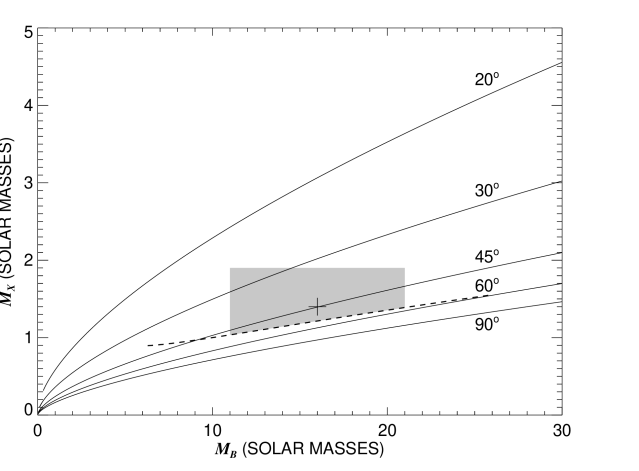
Figure 6: The relations between the supergiant mass $M_{B}$ and neutron star mass $M_{X}$ for LS I +65 010. Lines of constant orbital inclination are constructed from the mass function and are labeled at the right hand side. The dashed line indicates the upper limit on inclination and the lower limit on X-ray source mass based upon the lack of eclipses. The shaded region shows the probable solution space with the plus sign marking the favored solution.

We measured emission equivalent widths for H$\alpha$ by making a simple numerical integration of line flux above the continuum, and our results are listed in the final column of Table 2. The typical measurement errors are approximately $\pm 0.05$ Å for the higher dispersion spectra and about twice that for the lower dispersion spectra. The resulting equivalents widths fall within the range reported in the past (Reig et al., 1996; Liu & Hang, 1999). We searched for any periodic signals in the time variations of the H$\alpha$ equivalent widths using the discrete Fourier transform and CLEAN algorithm (Roberts, Lehár, & Dreher, 1987). These results are summarized for each observing season and for the entire data set in Figure 3. Most of the temporal variability appears to occur on timescales around 10 d (frequency of 0.1 cycles d^-1). We found no compelling evidence of periodic variability at either the orbital (11.6 d) or super-orbital period (30.7 d), and the $1\sigma$ upper limits for such cyclic variations are $<4\%$ and $<10\%$ for these two periods, respectively (based upon sinusoidal fits at these fixed periods). The strongest signal in the power spectrum (among a number of candidate periods in the range between 6 and 12 d) occurs at a period of $9.72\pm 0.02$ d. The false alarm probability that this peak is due to noise is small, $p_{0}\approx N\exp(-z_{0})=0.0002$ where $z_{0}=15.6$ is the ratio of the power peak to the variance and $N=1000$ is the number of quasi-independent frequencies tested over the range in physically interesting timescales between 0 and 1 cycle d^-1 (Scargle, 1982). Although H$\alpha$ variations occurred during each run on such timescales, there were large differences in the mean equivalent width between runs and in the detailed profile shape variations within runs that indicate the importance of other timescales as well. We suggest that this 10 d timescale represents a characteristic recurrence time for ephemeral structures to appear in a wind that is subject to longer term variations in mass loss rate. If the structures are azimuthally distributed with respect to the star’s spin axis, then this characteristic time may correspond to the stellar rotation period (see the case of the B-supergiant HD 64760 discussed by Fullerton et al. 1997 and the models for rotational modulation presented by Harries 2000). We can estimate the rotational period very approximately using the projected rotational velocity $V\sin i=96\pm 20$ km s^-1 and radius estimate $R/R_{\odot}=37\pm 15$ (Reig et al., 1996) plus the probable inclination range (see Fig. 6 below). The timescale for the H$\alpha$ variations falls within the derived range of rotational period of 9 to 15 d.

5 X-ray Variations

The 2S 0114+650 system is one of some hundred targets that have been under continuous surveillance since 1996 March by the All-Sky Monitor on the Rossi X-ray Timing Explorer (Levine et al., 1996). This instrument records the X-ray flux across three energy bands in 90 s observation segments. We extracted the flux measurements from 1996 March through 2006 May from the quick-look results provided by the RXTE/ASM team. The source is relatively weak and there is a significant amount of scatter among the individual measurements. However, since there are currently over 60,000 measurements available for 2S 0114+650, we can achieve a significant increase in S/N by averaging the fluxes into temporal or orbital-phase bins of interest.

We first consider the long term variations in X-ray flux. We show in the upper panel of Figure 4 the high energy band fluxes for the duration of the RXTE mission binned into intervals equivalent to 12 binary orbits (139 d). Each symbol shows the mean and standard deviation of the mean of the flux in the time bin. These means and errors were taken from measurements made only with the Scanning Shadow Camera (SSC) 2 and SSC3, since there is some indication of a long term trend of uncertain origin in the results from SSC1 for this particular source (possibly related to the calibration of gain changes in the proportional counter associated with SSC1). The lower panel illustrates the H$\alpha$ equivalent width measurements over the same dates (but with much more restricted time coverage). There is a significant range in observed equivalent width during each run (§4), but it appears that mean strength was largest in 1998 ($\sim$ HJD 2,451,060), smallest in 1999 ($\sim$ HJD 2,451,460), and intermediate in 2000 ($\sim$ HJD 2,451,860). The binned X-ray fluxes in the top panel also show a similar kind of variation, which is suggestive that the time-averaged H$\alpha$ emission and X-fluxes appear to vary together. Taken at face value, this indicates that long term variations in the B-supergiant mass loss rate are reflected in the X-ray accretion flux. A similar result was found for the massive X-ray binary and microquasar LS 5039 (Reig et al., 2003; McSwain et al., 2004).

Next we binned the ASM fluxes according to orbital phase from our spectroscopic solution (Table 3), and the light curves for the three energy bands are plotted in Figure 5. The orbital light curve is best defined in the 5 – 12 keV band where the observed counts are highest (top panel of Fig. 5; compare with the earlier light curve presented in Fig. 1 of Hall et al. 2000). We see that there is a clear maximum when the stars are closest near periastron (phase 0.0). At that point in the orbit, the neutron star will encounter the densest and slowest portions of the supergiant’s wind, and the wind accretion rate will attain a maximum (Lamers, van den Heuvel, & Petterson, 1976). The highest 5 – 12 keV flux average actually occurs for the bin centered at phase 0.08, corresponding to a time some 22 hours after periastron. This may indicate the interval between accretion and heating to X-ray emitting temperatures or it may represent the transit time for a wind density enhancement created by tidal effects at periastron to reach the vicinity of the neutron star.

The minimum in the X-ray light curve appears near phase 0.63, which is very close to the predicted phase of supergiant inferior conjunction at phase $0.65\pm 0.06$. The X-ray flux does not vanish at this minimum, so we suspect that we are observing an atmospheric rather than a total eclipse (Hall et al., 2000). For example, Wen et al. (1999) show that in the case of Cyg X-1, the decrease in X-ray flux observed when the supergiant is in the foreground is well explained by the attenuation of the X-ray flux by the wind of the supergiant. We suspect that the same explanation applies to the case of the LS I +65 010 = 2S 0114+650 system since Hall et al. (2000) find evidence of an increase in column density near X-ray minimum.

The kind of analysis made by Wen et al. (1999) of the wind attenuation as a function of orbital phase would also be profitable in this case and would presumably help place limits on the orbital inclination. We show in Figure 6 the constraints on the masses of the two components in the mass plane diagram. The solid lines show the mass relations for given values of orbital inclination that are derived from the mass function ($f(m)$ given in Table 3). Reig et al. (1996) estimate that the supergiant mass and radius are $16\pm 5~{}M_{\odot}$ and $37\pm 15~{}R_{\odot}$, respectively, based upon their analysis of the optical and near-IR spectrum. Note that this supergiant radius is much smaller than the star’s Roche radius for the full range of acceptable inclination and mass ratio. The limiting line for the absence of full eclipses is shown by the dashed line in Figure 6 (derived from the radius given above and the projected semimajor axis $a_{1}\sin i$ listed in Table 3). Finally, we can place a weak constraint on a minimum inclination angle of $i=20^{\circ}$ by assuming that the supergiant rotates no faster than the critical rate (based on the given radius and observed projected rotational velocity $V\sin i=96\pm 20$ km s^-1; Reig et al. 1996). This is a weak constraint because it is based upon the assumption that the supergiant’s spin inclination is the same as the orbital inclination, but these inclinations could differ if the neutron star suffered an asymmetric kick at the time of the supernova explosion (Brandt & Podsiadlowski, 1995). The shaded region in Figure 6 shows the probable B-supergiant range together with the observed range in neutron star mass (van Kerkwijk, van Paradijs, & Zuiderwijk, 1995), and a plus sign marks the nominal position for a Chandrasekhar mass neutron star ($1.4~{}M_{\odot}$). This best estimate solution has an inclination of $i=45^{\circ}$, just below eclipse limit near $i=50^{\circ}$, and this orientation is probably consistent with the atmospheric eclipse seen in the X-ray light curve. A realistic model of the X-ray attenuation by the wind of the B-supergiant would provide a reliable estimate of the inclination and better constraints on the masses of both stars.

Table 1: Journal of Optical Spectroscopy

Dates	Spectral Range	Resolving Power	Number
(HJD-2,400,000)	(Å)	($\lambda/\triangle\lambda$)	of Spectra
51053 – 51065	6313 – 6978	9530	23
51421 – 51429	5397 – 6735	4050	11
51464 – 51469	5400 – 6736	4100	14
51491 – 51497	5545 – 6881	4400	14
51817 – 51830	6440 – 7105	9500	16
51890 – 51901	6443 – 7108	9500	22

Table 2: Radial Velocity and Equivalent Width Measurements

Date	Orbital	$V_{r}$	$(O-C)$	$\triangle V_{\rm ISM}$	$W_{\lambda}({\rm H}\alpha)$
(HJD$-$2,400,000)	Phase	(km s-1)	(km s-1)	(km s-1)	(Å)
51053.803	0.481	$-70.8$	0$-4.5$	0$-1.8$	$-$2.05
51053.824	0.483	$-66.8$	0$-0.5$	0$-0.4$	$-$2.01
51055.810	0.655	$-55.1$	0+$1.1$	0+$0.6$	$-$1.98
51055.832	0.656	$-56.3$	0$-0.2$	0+$0.7$	$-$2.10
51055.917	0.664	$-53.9$	0+$1.8$	0+$3.9$	$-$2.02
51056.826	0.742	$-56.1$	0$-6.0$	0+$2.4$	$-$1.70
51056.850	0.744	$-54.4$	0$-4.5$	0+$2.3$	$-$1.68
51056.871	0.746	$-57.0$	0$-7.3$	0+$2.2$	$-$1.74
51057.810	0.827	$-50.5$	0$-5.8$	0+$1.0$	$-$1.53
51057.831	0.829	$-49.7$	0$-5.2$	0+$2.0$	$-$1.59
51057.852	0.831	$-49.7$	0$-5.3$	0+$2.1$	$-$1.66
51058.801	0.912	$-47.0$	0$-4.4$	0+$3.6$	$-$1.15
51058.822	0.914	$-49.8$	0$-7.1$	0+$2.8$	$-$1.16
51058.844	0.916	$-49.2$	0$-6.5$	0+$2.4$	$-$1.28
51061.800	0.171	$-61.0$	0+$5.0$	0$-2.0$	$-$1.77
51061.821	0.173	$-57.6$	0+$8.6$	0$-0.1$	$-$1.77
51061.843	0.175	$-59.2$	0+$7.1$	0+$2.3$	$-$1.73
51063.887	0.351	$-73.2$	0$-2.9$	0+$2.0$	$-$1.11
51063.908	0.353	$-71.4$	0$-1.0$	0+$1.7$	$-$1.13
51063.930	0.355	$-74.6$	0$-4.3$	0+$0.5$	$-$1.17
51065.811	0.517	$-71.5$	0$-6.9$	0+$0.5$	$-$1.54
51065.835	0.519	$-66.0$	0$-1.5$	0$-0.5$	$-$1.63
51065.856	0.521	$-64.4$	0+$0.0$	0+$0.7$	$-$1.75
51421.915	0.220	$-69.0$	0$-0.2$	0$-3.2$	$-$0.98
51423.896	0.391	$-75.5$	0$-5.9$	0$-3.2$	$-$1.30
51425.898	0.563	$-68.8$	0$-6.7$	0$-6.6$	$-$1.27
51425.919	0.565	$-67.4$	0$-5.4$	0$-7.9$	$-$1.28
51426.879	0.648	$-61.4$	0$-4.7$	0$-0.4$	$-$0.82
51426.901	0.650	$-60.9$	0$-4.3$	0$-0.2$	$-$0.85
51427.879	0.734	$-56.3$	0$-5.7$	0+$1.2$	$-$0.86
51428.838	0.817	$-48.2$	0$-3.1$	0$-1.8$	$-$0.79
51428.860	0.819	$-48.7$	0$-3.6$	0$-1.1$	$-$0.82
51429.836	0.903	$-46.1$	0$-3.5$	0$-1.5$	$-$0.93
51429.857	0.905	$-46.4$	0$-3.8$	0+$1.0$	$-$0.90
51464.760	0.914	$-44.5$	0$-1.8$	0$-0.3$	$-$1.43
51464.783	0.916	$-41.9$	0+$0.9$	0+$1.0$	$-$1.17
51465.814	0.005	$-57.9$	0$-9.7$	0$-3.8$	$-$1.57
51465.835	0.007	$-56.0$	0$-7.6$	0$-5.6$	$-$1.63
51465.858	0.009	$-57.5$	0$-8.8$	0$-4.0$	$-$1.50
51466.772	0.087	$-56.0$	0+$1.9$	0$-8.4$	$-$1.28
51466.794	0.089	$-57.1$	0+$1.1$	0$-5.2$	$-$1.26
51466.816	0.091	$-59.0$	0$-0.6$	0$-3.4$	$-$1.35
51467.855	0.181	$-72.7$	0$-5.9$	0$-0.4$	$-$1.03
51467.876	0.183	$-70.7$	0$-3.9$	0$-2.2$	$-$1.19
51468.812	0.263	$-70.9$	0$-0.7$	0+$1.3$	$-$1.46
51468.834	0.265	$-65.4$	0+$4.8$	0+$0.8$	$-$1.49
51469.829	0.351	$-67.6$	0+$2.8$	0$-6.1$	$-$1.28
51469.850	0.353	$-70.5$	0$-0.2$	0$-2.1$	$-$0.72
51491.753	0.241	$-56.9$	+$12.7$	0$-2.9$	$-$1.56
51491.775	0.243	$-58.0$	+$11.7$	$\cdots$	$-$1.64
51492.713	0.324	$-64.2$	0+$6.5$	0+$3.0$	$-$1.70
51492.734	0.326	$-69.8$	0+$0.8$	0$-0.8$	$-$1.66
51493.696	0.409	$-71.9$	0$-2.8$	0+$3.0$	$-$1.46
51493.717	0.411	$-73.0$	0$-3.9$	0+$3.4$	$-$1.43
51494.708	0.496	$-60.3$	0+$5.4$	0$-2.3$	$-$1.14
51494.730	0.498	$-58.9$	0+$6.7$	0$-4.5$	$-$1.22
51495.765	0.587	$-62.5$	0$-1.9$	0+$1.1$	$-$0.91
51495.787	0.589	$-58.9$	0+$1.6$	0+$1.1$	$-$0.89
51496.757	0.673	$-66.3$	$-11.3$	0$-4.3$	$-$0.95
51496.778	0.675	$-66.2$	$-11.3$	0$-4.1$	$-$0.46
51497.718	0.756	$-55.6$	0$-6.5$	0$-2.5$	$-$0.87
51497.739	0.757	$-56.4$	0$-7.4$	0$-1.6$	$-$0.81
51817.702	0.344	$-69.6$	0+$0.8$	0$-1.0$	$-$1.13
51817.739	0.348	$-70.3$	0+$0.2$	0$-1.9$	$-$1.20
51818.722	0.432	$-64.1$	0+$4.2$	0$-1.0$	$-$1.16
51818.746	0.434	$-68.3$	0$-0.0$	0+$0.3$	$-$1.14
51819.693	0.516	$-59.7$	0+$5.0$	0+$1.0$	$-$1.10
51819.716	0.518	$-59.9$	0+$4.7$	0$-2.4$	$-$1.02
51820.735	0.606	$-56.3$	0+$3.2$	0$-0.0$	$-$1.21
51821.698	0.689	$-52.1$	0+$1.7$	0$-0.6$	$-$1.20
51821.720	0.691	$-52.5$	0+$1.2$	0$-1.5$	$-$1.24
51822.710	0.776	$-24.2$	+$23.5$	0+$1.3$	$-$1.21
51823.692	0.861	$-22.2$	+$21.1$	0+$0.2$	$-$1.65
51823.713	0.863	$-21.0$	+$22.2$	0+$0.7$	$-$1.56
51824.687	0.947	$-42.9$	0+$0.8$	0+$3.7$	$-$1.32
51824.708	0.949	$-43.8$	0+$0.1$	0+$4.1$	$-$1.30
51830.713	0.466	$-64.5$	0+$2.5$	0$-1.2$	$-$1.89
51830.735	0.468	$-65.0$	0+$1.9$	0+$0.2$	$-$1.75
51890.622	0.632	$-65.4$	0$-7.6$	0$-2.0$	$-$1.81
51890.643	0.633	$-66.2$	0$-8.5$	0+$0.8$	$-$1.86
51892.613	0.803	$-45.3$	0+$0.6$	0$-2.9$	$-$1.86
51892.635	0.805	$-45.1$	0+$0.8$	0$-1.4$	$-$1.76
51893.642	0.892	$-43.0$	0$-0.4$	0$-0.3$	$-$1.39
51893.664	0.894	$-43.0$	0$-0.4$	0+$0.0$	$-$1.34
51894.640	0.978	$-51.1$	0$-5.4$	0$-2.0$	$-$1.42
51894.661	0.980	$-51.5$	0$-5.5$	0$-0.5$	$-$1.33
51895.620	0.063	$-60.5$	0$-5.5$	0$-0.7$	$-$1.51
51895.642	0.064	$-59.4$	0$-4.2$	0$-0.1$	$-$1.49
51896.662	0.152	$-70.3$	0$-5.7$	0$-0.5$	$-$1.07
51896.683	0.154	$-70.9$	0$-6.2$	0+$0.5$	$-$1.24
51897.664	0.239	$-67.1$	0+$2.5$	0$-1.5$	$-$1.15
51897.685	0.241	$-69.6$	0+$0.0$	0$-0.6$	$-$1.10
51898.667	0.325	$-72.0$	0$-1.4$	0$-1.6$	$-$1.47
51898.688	0.327	$-72.6$	0$-2.0$	0$-1.4$	$-$1.50
51899.670	0.412	$-73.0$	0$-4.0$	0+$0.3$	$-$1.70
51899.691	0.413	$-74.5$	0$-5.5$	0$-1.0$	$-$1.74
51900.664	0.497	$-55.9$	0+$9.7$	0+$1.0$	$-$1.67
51900.685	0.499	$-54.2$	+$11.3$	0+$1.6$	$-$1.64
51901.649	0.582	$-44.9$	+$16.0$	0+$1.2$	$-$1.31
51901.671	0.584	$-48.4$	+$12.5$	0$-1.1$	$-$1.45

Table 3: Orbital Elements

Element	Crampton et al. (1985)	This Work
$P$ (days)	$11.588\pm 0.003$	$11.5983\pm 0.0006$
$T$ (HJD–2,400,000)	$44134.9\pm 0.7$	$51825.3\pm 0.5$
$e$	$0.16\pm 0.07$	$0.18\pm 0.05$
$\omega$ (deg)	$11\pm 11$	$51\pm 17$
$K$ (km s-1)	$17\pm 1$	$14.0\pm 0.7$
$\gamma$ (km s-1)	$-57\pm 1$	$-58.2\pm 0.5$
$f(m)$ ($M_{\odot}$)	$0.006\pm 0.001$	$0.0032\pm 0.0005$
$a_{1}\sin i$ ($R_{\odot}$)	$3.9\pm 0.2$	$3.16\pm 0.16$
r.m.s. (km s-1)	$6.8$	$6.4$

Figure 1: Calculated radial velocity curve (solid line) for LS I +65 010. The measured radial velocities are shown as filled circles. Open circles mark the measurements that were assigned zero weight (§3), and plus signs indicate the measurements from Crampton et al. (1985).

Figure 2: Temporal variations in the H$\alpha$ profile. The left panel shows the profiles from 1998 August while the right panel shows the variations in 2000 December. The vertical bar at upper right indicates the spectral intensity scale relative to a unit continuum. The spectra were smoothed with a Gaussian filter with FWHM = 30 km s^-1.

Figure 3: Periodograms of the H$\alpha$ equivalent width variations for data from 1998, 1999, 2000, and all years (top to bottom, with offsets of 0.6, 0.45, 0.3, and 0.15, respectively). The lower plot shows the CLEANed periodogram (offset by 0.05) derived from a deconvolution of the full sample periodogram.

Figure 4: The long term variations in the RXTE/ASM high energy flux and H$\alpha$ equivalent width. The top panel shows the ASM counts binned into intervals of 139 d (12 orbital periods) while the lower panel illustrates the H$\alpha$ emission strength. The plus signs indicate our measurements while the single $\times$ sign is based on the observation from Koenigsberger et al. (2003).

Figure 5: The RXTE/ASM fluxes binned according to orbital phase (phase 0.0 for periastron). The panels show the bin mean and standard deviation of the mean of ASM counts for each of the three energy bands.

References

- Bonning & Falanga (2005) Bonning, E. W., & Falanga, M. 2005, A&A, 436, L31
- Brandt & Podsiadlowski (1995) Brandt, N., & Podsiadlowski, Ph. 1995, MNRAS, 274, 461
- Coe (2000) Coe, M. J. 2000, in The Be Phenomenon in Early-Type Stars, IAU Coll. 175 (ASP Conf. Vol. 214), ed. M. A. Smith, H. F. Henrichs, & J. Fabregat (San Francisco: ASP), 656
- Crampton et al. (1985) Crampton, D., Hutchings, J. B., & Cowley, A. P. 1985, ApJ, 299, 839
- Farrell et al. (2006) Farrell, S. A., Sood, R. K., & O’Neill, P. M. 2006, MNRAS, 367, 1457
- Finley et al. (1992) Finley, J. P., Belloni, T., & Cassinelli, J. P. 1992, A&A, 262, L25
- Fullerton et al. (1997) Fullerton, A. W., Massa, D. L., Prinja, R. K., Owocki, S. P., & Cranmer, S. R. 1997, A&A, 327, 699
- Gies & Bolton (1986) Gies, D. R., & Bolton, C. T. 1986, ApJS, 61, 419
- Gies et al. (2003) Gies, D. R., et al. 2003, ApJ, 583, 424
- Grundstrom et al. (2006b) Grundstrom, E. D., Finch, C., Gies, D. R., Huang, W., McSwain, M. V., O’Brien, D. P., Riddle, R. L., Trippe, M. L., & Wingert, D. W., & Zaballa, R. A. 2006b, ApJ, submitted
- Grundstrom et al. (2006a) Grundstrom, E. D., et al. 2006a, ApJ, submitted
- Hall et al. (2000) Hall, T. A., Finley, J. P., Corbet, R. H. D., & Thomas, R. C. 2000, ApJ, 536, 450
- Harries (2000) Harries, T. J. 2000, MNRAS, 315, 722
- Kaper (1998) Kaper, L. 1998, in Boulder-Munich II: Properties of Hot, Luminous Stars (ASP Conf. Vol. 131), ed. I. Howarth (San Francisco: ASP), 427
- Koenigsberger et al. (2003) Koenigsberger, G., Canalizo, G., Arrieta, A., Richer, M. G., & Georgiev, L. 2003, Rev. Mexicana Astron. Astrofis., 39, 17
- Lamers et al. (1976) Lamers, H. J. G. L. M., van den Heuvel, E. P. J., & Petterson, J. A. 1976, A&A, 49, 327
- Levine et al. (1996) Levine, A. M., Bradt, H., Cui, W., Jernigan, J. G., Morgan, E. H., Remillard, R., Shirey, R. E., & Smith, D. A. 1996, ApJ, 469, L33
- Li & van den Heuvel (1999) Li, X. D., & van den Heuvel, E. P. J. 1999, ApJ, 513, L45
- Liu & Hang (1999) Liu, Q.-Z., & Hang, H.-R. 1999, A&A, 350, 855
- Lucy & Sweeney (1971) Lucy, L. B., & Sweeney, M. A. 1971, AJ, 76, 544
- Markova & Valchev (2000) Markova, N., & Valchev, T. 2000, A&A, 363, 995
- McSwain et al. (2004) McSwain, M. V., Gies, D. R., Huang, W., Wiita, P. J., Wingert, D. W., & Kaper, L. 2004, ApJ, 600, 927
- Morbey & Brosterhus (1974) Morbey, C., & Brosterhus, E. B. 1974, PASP, 86, 455
- Reig et al. (1996) Reig, P., Chakrabarty, D., Coe, M. J., Fabregat, J., Negueruela, I., Prince, T. A., Roche, P., & Steele, I. A. 1996, A&A, 311, 879
- Reig et al. (2003) Reig, P., Ribó, M., Paredes, J. M., & Martí, J. 2003, A&A, 405, 285
- Roberts et al. (1987) Roberts, D. H., Lehár, J., & Dreher, J. W. 1987, AJ, 93, 968
- Scargle (1982) Scargle, J. D. 1982, ApJ, 263, 835
- van Kerkwijk et al. (1995) van Kerkwijk, M. H., van Paradijs, J., & Zuiderwijk, E. J. 1995, A&A, 303, 497
- Wen et al. (1999) Wen, L., Cui, W., Levine, A. M., & Bradt, H. V. 1999, ApJ, 525, 968
- Wen et al. (2006) Wen, L., Levine, A. M., Corbet, R. H. D., & Bradt, H. V. 2006, ApJS, 163, 372