The Luminosity Function and Star Formation Rate between Redshifts of 0.07 and 1.47 for Narrow-band Emitters in the Subaru Deep Field

Abstract

Subaru Deep Field line-emitting galaxies in four narrow-band filters (NB704, NB711, NB816, and NB921) at low and intermediate redshifts are presented. Broad-band colors, follow-up optical spectroscopy, and multiple narrow-band filters are used to distinguish H$\alpha$, [O ii], and [O iii] emitters between redshifts of 0.07 and 1.47 to construct their averaged rest-frame optical-to-UV spectral energy distributions and luminosity functions. These luminosity functions are derived down to faint magnitudes, which allows for a more accurate determination of the faint end slope. With a large (N $\sim$ 200 to 900) sample for each redshift interval, a Schechter profile is fitted to each luminosity function. Prior to dust extinction corrections, the [O iii] and [O ii] luminosity functions reported in this paper agree reasonably well with those of Hippelein et al. The $z=0.08$ H$\alpha$ LF, which reaches two orders of magnitude fainter than Gallego et al., is steeper by 25%. This indicates that there are more low luminosity star-forming galaxies for $z<0.1$. The faint end slope $\alpha$ and $\phi_{\star}$ show a strong evolution with redshift while $L_{\star}$ show little evolution. The evolution in $\alpha$ indicates that low-luminosity galaxies have a stronger evolution compared to brighter ones. These results can only be achieved with deep NB observations over a wide range in redshift. Integrated star formation rate densities are derived via H$\alpha$ for $0.07<z<0.40$, [O iii] for $0.40<z<0.84$, and [O ii] for $0.89<z<1.47$. A steep increase in the star-formation rate density, as a function of redshift, is seen for $0.4\lesssim z\lesssim 0.9$. For $z\gtrsim 1$, the star-formation rate densities are more or less constant. The latter is consistent with previous UV and [O ii] measurements. Below $z\lesssim 0.4$, the SFR densities are consistent with several H$\alpha$, [O ii], and UV measurements, but other measurements are a factor of two higher. For example, the $z=0.066-0.092$ H$\alpha$ LF agrees with those of Jones & Bland-Hawthorn, but at $z=0.24$ and 0.40, their number density is higher by a factor of two. This discrepancy can be explained by cosmic variance.

1. INTRODUCTION

Over the past decade, deep spectroscopic surveys have utilized emission lines to measure the cosmic star-formation rate (SFR). Estimates of the SFR can be obtained from the H$\alpha$ emission line in star-forming galaxies (Kennicutt, 1983). However, H$\alpha$ is no longer visible (in optical spectrographs) beyond $z\,\sim\,0.4$. To study the SFR at higher redshifts, one must obtain infrared spectroscopy of the H$\alpha$ line or detect bluer emission lines where optical spectrographs are used. Although the former has been successful (e.g., Malkan et al., 1995; Glazebrook et al., 1999; McCarthy et al., 1999; Yan et al., 1999; Hopkins et al., 2000; Moorwood et al., 2000; Tresse et al., 2002; Doherty et al., 2006; Rodriguez-Eugenio et al., 2006), difficulties, such as a bright background (for ground-based observations) and smaller areal coverage limit IR searches to small samples, mostly of the brightest galaxies.

The latter has been attempted by measuring the O ii doublet ([O ii] $\lambda\lambda$3726, 3729). It has been used to determine the SFR out to $z$ = 1.6 (Hogg et al., 1998; Hicks et al., 2002; Hippelein et al., 2003; Teplitz et al., 2003; Drozdovsky et al., 2005), but its measurements are more affected by internal extinction and metallicity uncertainties (Kennicutt, 1992; Kewley, Gellar, & Jansen, 2004). Studies have shown that the comoving SFR density increases by a factor of 10 from $z\sim 0$ to 1-1.5 and declines or flattens out at higher redshifts (Hopkins, 2004). The behavior above a redshift of 3 is not well known for two reasons: ($i$) the amount of UV extinction is questionable, and ($ii$) the shallowness of recent Lyman Break Galaxies studies at $z>5$ has resulted in an extrapolation of the faint-end slope for a SFR estimate.

Since past studies identified galaxies and redshifts via spectra, the measured SFRs are biased toward the small selected sample of bright objects, and spectroscopy requires a greater demand of allocated telescope time, as opposed to the approach of using deep narrow-band (NB) imaging with large fields-of-view. The NB imaging method has proven to be quite effective in finding many emission line galaxies with the appropriate redshift for a strong line (e.g., Ly$\alpha$, H$\alpha$, [O ii] $\lambda$3727, H$\beta$, and [O iii] $\lambda$5007) to fall within the NB filter. For example, Hu et al. (2002), Ajiki et al. (2003), Kodaira et al. (2003), Taniguchi et al. (2003), Hu et al. (2004), Kashikawa et al. (2006), and Shimasaku et al. (2006) have confirmed candidate Ly$\alpha$ emitters (LAEs) at $z=5.7$ and 6.6 with follow-up spectroscopy. These NB emitters (identified when their NB magnitude is substantially brighter than that of the broad-band continuum) provide an opportunity to study the cosmic evolution of star formation. Fujita et al. (2003), Kodama et al. (2004), and Umeda et al. (2004) have measured the H$\alpha$ luminosity function (the latter two are for clusters) at $z$ = 0.24 or 0.40 by identifying NB emitters and then using their broad-band colors to distinguish a few hundred H$\alpha$ emitters from other line emitters. Ajiki et al. (2006) also examined the same field as Fujita et al. (2003) for other strong emission line galaxies such as [O iii] and [O ii]. Fabry-Perot (FP) interferometers have also been used to find emission line galaxies (Jones & Bland-Hawthorn, 2001; Hippelein et al., 2003; Glazebrook et al., 2004), but the comoving volume or limiting flux of past surveys is not comparable to that of the NB imaging technique, and their surveys currently lack broad-band colors. Other work, such as COMBO-17 (Meisenheimer & Wolf, 2002) that uses intermediate-band filters is capable of selecting emission line galaxies, but these wider filters (compared to NBs) will only detect very strong line emitting galaxies.

In this paper, the luminosity function (LF) and SFR in almost a dozen redshift windows between $z$ = 0.07 and 1.47 are presented from line-emitting galaxies in the Subaru Deep Field (SDF; Kashikawa et al., 2004). The approach of using broad-band colors to separate NB emitters will be considered. However, with spectra of some of our NB emitters, galaxies (with appropriate redshifts) from the Hawaii HDF-N (a deep spectroscopic survey), and multiple NB filters to cover two different lines at similar redshifts, the LF for line emitters other than the typical H$\alpha$ and Ly$\alpha$ can be studied. Broad-band (BB) multi-color selection of [O ii] and [O iii] emitters has yet to be done at these intermediate redshifts. The combination of deep, wide imaging with multiple broad- and narrow-band filters makes the SDF scientifically unique. In § 2, deep broad- and narrow-band imaging are presented. Selection criteria for different NB emitters are described and follow-up spectroscopy of the brightest line-emitting galaxies are also presented in § 2. Section 3 will discuss our methods of distinguishing different line emitters, derive emission line fluxes from NB photometry, calculate the luminosity function, and derive SFRs at 11 redshift windows. Comparisons with previous studies will be made in § 4, and a discussion of the evolution of the luminosity function and star formation rate density, and suggestions for future work are given in § 5. Concluding remarks are made in the final section.

A flat cosmology with H_∘ = 70 km s^-1 Mpc^-1, $\Omega_{\Lambda}$ = 0.7, and $\Omega_{M}$ = 0.3 is adopted for consistency with recent papers related to this topic and cosmological measurements (Spergel et al., 2003, 2006). Throughout this paper, all magnitudes are given in the AB system: $m_{\rm AB}=-2.5\log{f_{\nu}}-48.60$, where $f_{\nu}$ is the flux density in ergs s^-1 cm^-2 Hz^-1.

2. OBSERVATIONS

2.1. Optical Imaging

Deep optical imaging of the SDF (centered at 13^h24^m38$\fs$9, +27°29′25$\farcs$9) has been obtained with Suprime-Cam on the 8.2-m Subaru Telescope (Kaifu, 1998; Iye et al., 2004). Five broad-band ($B$, $V$, $R_{\rm C}$, $i$′, and $z$′) and four narrow-band (NB704, NB711, NB816, and NB921) images were obtained with a total integration time of 595, 340, 600, 801, 504, 198, 162, 600, and 899 minutes, respectively. The NB704 and NB711 images were part of a LAE study at $z\,\simeq\,5$ taken in 2001 March-June and 2002 May before the SDF project began (Ouchi et al., 2003; Shimasaku et al., 2003, 2004). The remaining data were obtained as part of the SDF project. The limiting magnitudes (3$\sigma$ with a 2″-aperture) for each 27′ $\times$ 34′ image are ($B$) 28.45, ($V$) 27.74, ($R_{\rm C}$) 27.80, ($i$′) 27.43, ($z$′) 26.62, (NB704) 26.67, (NB711) 25.99, (NB816) 26.63, and (NB921) 26.54. The correction for galactic reddenning is small, $E(B-V)$ = 0.017 (Schlegel, Finkbeiner, & Davis, 1998). Each image contains over 100,000 objects. After removing regions of low quality (the edges of the CCD and saturated regions around foreground stars), the effective field-of-view is about 868 sq. arcmin. Catalogs for each bandpass were constructed using Source Extractor v2.1.6 (SExtractor; Bertin & Arnouts, 1996).

This paper will only discuss low and intermediate redshift NB704, NB711, NB816, and NB921 emitters. High redshift LAEs in the SDF are discussed in Kodaira et al. (2003), Ouchi et al. (2003), Shimasaku et al. (2003, 2004), Taniguchi et al. (2005), Kashikawa et al. (2006), and Shimasaku et al. (2006).

2.1.1 NB704, NB711, NB816, and NB921 Line Emitters

BB-NB excess diagrams for the NB704, NB711, NB816, and NB921 catalogs are shown in Figures 1a-d for NB magnitudes up to the 3$\sigma$ limiting magnitude. The NB704, NB711, NB816, and NB921 excesses are described by $Ri$′ - NB704, $Ri$′ - NB711, $i$′$z$′ - NB816, and $z$′ - NB921, respectively, where $Ri$′ = $\text@frac{1}{2}$($R_{\rm C}+i$′) and $i$′$z$′ = 0.6$i$′ + 0.4$z$′. The limiting magnitude of $Ri$′ is 27.62 and 27.11 for $i$′$z$′. Objects above the short-long dashed magenta lines in Figure 1a-d are fainter than 3$\sigma$ of their broad-band flux ($Ri$′, $i$′$z$′, or $z$′). The median (i.e., featureless spectra) for the NB816 and NB921 excesses are 0.10 and -0.05 mag, respectively. NB line emitters are identified as points above the long-dashed blue (a minimum NB excess) and solid red lines in Figure 1. The solid red lines represent the $3\sigma$ excess: $\pm 3\sigma_{\rm BB-NB}=-2.5\log{[1\mp(f_{3\sigma NB}^{2}+f_{3\sigma BB}^{2})^{0.5}/f_{NB}]}$, where the error $[f_{3\sigma NB}^{2}+f_{3\sigma BB}^{2}]^{0.5}$ is shown in the upper right-hand corners of Figures 1a-d. The minimum NB excesses were chosen ‘by eye’ to be above the NB-BB scatter around NB of 23 mag.

These selection criteria yield 1135 NB704, 1068 NB711, 1916 NB816, and 2135 NB921 line emitters. These values are reduced to 1000, 986, 1563, and 1942 with good photometric errors ($\Delta m<0.1$) for broad-band filters used in the color selections (see §§§ 3.1.1-3.1.3). These line excess limits reach similar equivalent widths (see §§ 3.3) as Fujita et al. (2003) and Umeda et al. (2004).

2.2. Spectral Identification of NB Emitters

H$\alpha$ and [O iii] NB emitters are the easiest to be identified in an optical spectrum. H$\alpha$ emitters can be confirmed from detection of other strong lines, [O iii] and H$\beta$. And in cases (NB816 emitters) where the spectrum is truncated, the [N ii] $\lambda\lambda$6548, 6583 and [S ii] $\lambda\lambda$6718, 6732 doublet can be used. [O iii] emitters are easily confirmed by the presence of its doublet feature, and H$\beta$ for some objects. Also, for some NB921 [O iii] emitters, the [O ii] doublet appears on the blue side of the spectrum. Ly$\alpha$ and [O ii] emitters are difficult to distinguish since the nearest lines are either weak ([Ne iii] $\lambda$3869, H$\delta$, and H$\gamma$) or are AGN lines (C iv, [Ne iii] $\lambda$3869), and low spectral resolution cannot resolve the very close [O ii] doublet (e.g., FOCAS; DEIMOS can resolve the doublet). However, Ly$\alpha$ appears asymmetric at high redshifts, and are undetected in $B$ and $V$ for NB704, NB711, and NB816 emitters, and $B$, $V$, $R_{\rm C}$, and $i\arcmin$ for NB921 emitters. Therefore, the asymmetry of the line and broad-band detection can be used to distinguish [O ii] and Ly$\alpha$ (Kashikawa et al., 2006; Shimasaku et al., 2006).

2.3. Previous Subaru/FOCAS Spectroscopy

Faint Object Camera and Spectrograph (FOCAS; Kashikawa et al., 2002) observations primarily targeting NB816 and NB921 emitters were made on 2002 June 7-10, 2003 June 5-8, and 2004 April 24-27. The description of these observations can be found in Kodaira et al. (2003), Taniguchi et al. (2005), Kashikawa et al. (2006), and Shimasaku et al. (2006). A total of 24 LAEs, 4 [O ii], and 4 [O iii] NB816 emitters were identified with FOCAS. For NB921 emitters, 11 LAEs, 19 [O iii], and 1 H$\alpha$ were identified. These observations were intended to target LAEs, but a range in broad-band colors were allowed to determine the selection effects of a color-selected sample. The photometric and redshift information for non-LAEs are provided in Table 1, and Figure 2 shows the spectrum of NB921 emitters with line fluxes (ordinate) plotted in ergs s^-1 cm^-2 Å^-1. The sky’s spectrum is plotted at the top with arbitrary units. The spectra of NB816 emitters can be found in Shimasaku et al. (2006), so they are not reproduced. In addition, these NB emitters are plotted as open circles in Figure 1 and other figures. The convention throughout this paper is that red, green, and blue points are H$\alpha$, [O iii]/H$\beta$, and [O ii] emitters, respectively. Eight NB816 emitters and eight NB921 emitters remain unclear (either Ly$\alpha$ or [O ii]).

Moreover, deeper broad-band observations have revealed that three NB711 emitters published in Shimasaku et al. (2003) appear to be [O ii] emitters by detection in the $B$ and $V$ filters, but a chance projection of a foreground object cannot be ruled out. These sources are listed at the end of Table 1.

2.4. DEIMOS Spectroscopy of NB816 and NB921 Emitters

Deep Imaging Multi-Object Spectrograph (DEIMOS; Faber et al., 2003) observations were made on 2004 April 23 and 24 on Keck II. A total of four masks were used with an 830 lines mm^-1 grating and a GG495 order-cut filter. Each mask had an integration time of 7 - 9 kiloseconds, and had about 100 slits with widths of 1$\farcs$0 (0.47Å pix^-1, R $\sim 3600$ at 8500Å). The typical seeing for these observations was 0$\farcs$5 - 1$\farcs$0. Standard stars BD +28° 4211 and Feige 110 (Oke, 1990) were observed for the flux calibration. The second mask was flux calibrated with BD +28° 4211, and the other three masks were calibrated with Feige 110. All DEIMOS observations were reduced in the standard manner with the spec2d pipeline. A total of 33 NB816 and 21 NB921 known line emitters (including LAEs) were targeted with DEIMOS. NB816 emitters were selected for having $i$′ - NB816 $\geq$ 1.0 and 20.0 $\leq$ NB816 $\leq$ 25.5 (8.5$\sigma$), and NB921 emitters were selected for $z$′ - NB921 $\geq$ 1.0 and 20.0 $\leq$ NB921 $\leq$ 25.5 (7.8$\sigma$). These criteria were used to identify the brightest line emitters in the sample.

Among the NB816 and NB921 line emitters that have been targeted, 4 [O ii] $z$ = 1.47, 4 [O ii] $z$ = 1.19, 3 [O iii] $z$ = 0.84, 6 [O iii] $z$ = 0.63, 1 H$\alpha$ $z$ = 0.40, and 1 H$\alpha$ emitter at $z$ = 0.24 have been newly identified. Their redshift and photometric information are also provided in Table 1. The flux-calibrated spectra of these sources are shown in Figure 3. For Figure 2 and 3, vertical red lines represent the location of emission lines at the given redshift. For [O ii] emitters, the red lines are for a rest wavelength of 3726Å and 3729Å. While for [O iii] emitters, the lines are 4959Å and 5007Å. In the case of the H$\alpha$ emitters, the bluer part (adjacent panel to the left) of the spectrum has been included to show the [O iii] lines. Red lines near H$\alpha$ are the expected location of the [N ii] doublet. The number of new LAEs at $z$ = 5.70 $\pm$ 0.05 and $z$ = 6.56 $\pm$ 0.05 is 10 and 5, respectively. They are published in Shimasaku et al. (2006) and Kashikawa et al. (2006).

2.4.1 Spectroscopy of ‘Serendipitous’ and ‘Fortuitous’ Sources

Because of the long (up to 10″) DEIMOS slits, other galaxies falling within the slits are identified by the reduction pipeline as ‘serendipitous’. Moreover, other lower priority sources targeted with DEIMOS yield redshifts in the same range as those of the NB filters. These ‘fortuitous’ and serendipitous sources may not satisfy our NB excess selection criterion in §§ 2.1.1 or have any emission lines (some are identified via absorption features), but they provide important information about the broad-band colors at these redshifts. There are five serendipitous sources with relevant redshifts: three $z\approx 0.83$ [O iii] and two $z\approx 1.46$ [O ii] that are included in this paper. They are plotted as filled squares in Figure 1 and subsequent figures, and are listed in Table 1. Twenty fortuitous sources are identified, and are included in Table 1. The spectra of the fortuitous sources are shown in Figure 4, and are identified in NB-excess, and two-color figures as filled triangles.

Therefore, the total (including serendipitous and fortuitous sources) number of spectra that will be used in our line classification scheme is 75. Table 2 summarizes the number of spectroscopically-identified sources within different redshift windows.

2.5. NB Excess Predictions from Sloan Digital Sky Survey

Mean spectra for six galaxy types (from early to late) were obtained from Yip et al. (2004) and were then redshifted for either H$\alpha$, [O iii], or [O ii] to fall within the four NB filters and then convolved with the BB and NB filters. The spectra were averaged over 100 to 20000 Sloan Digital Sky Survey (SDSS) sources. This procedure tests whether or not typical galaxies detected in the SDSS are capable of being detected in the NB filters due to strong emission lines. The BB-NB excesses for the three latest types (Sbc/Sc, Sm/Im, and SBm) are shown as horizontal lines on the left-hand side of Figure 1a-d. The BB-NB excess method shows that the two latest types (Sm/Im and SBm) can easily be detected with NB filters due to their very strong emission lines, and Sbc/Sc can be detected in some cases. The Sm/Im and SBm galaxies make up 0.5% of the entire sample of Yip et al. (2004), and the Sbc/Sc sample consists of 23%. Thus at low redshift, for example, our NB imaging would detect about a quarter of the SDSS galaxies.

3. RESULTS

Multiple possibilities exist for the identification of a detected emission line in a NB filter. Ly$\alpha$, [O ii] $\lambda$3727, H$\beta$, [O iii] $\lambda\lambda$4959, 5007, and H$\alpha$ are the strongest lines that most likely will be identified. The spectra of NB strong emitters show that they are either H$\alpha$, [O iii], or [O ii]; neither of them are H$\beta$. Other objects (serendipitous and fortuitous) with H$\beta$ in the filter have very low NB-BB excess. It is therefore assumed that these NB emitters are more likely to have [O iii] rather than H$\beta$. The redshift range, comoving volume, and luminosity distance ($d_{L}$) are listed in Table 3 for all four NB filters.

3.1. Broad-band Color Selection

Past studies (e.g., Fujita et al., 2003; Kodama et al., 2004; Umeda et al., 2004) that have used multi-color spectral energy distributions (SEDs) of NB emitters, relied on theoretical population synthesis models to identify photometric H$\alpha$ emitters. However, without spectra of a sample of bright galaxies, the identification of these emitters cannot be confirmed. Since spectra have been obtained for a few to over two dozen objects in each redshift bin, the multi-color classification of different ([O ii] and [O iii]) line emitters in this study is more reliable than previous studies. With five broad bandpasses, distinguishing different line emitters is more feasible in a multidimensional color space, as previous studies were limited to two or three broad bandpasses. Many of the colors that will be used rely on the Balmer break falling in a particular bandpass.

The NB704 filter provides the special advantage of determining the redshift of NB921 emitters into two possible intervals. This is almost equivalent to obtaining a spectra, as a line-emitting galaxy in the NB704 and NB921 filters correspond to either a redshift of 0.397-0.411 or 0.878-0.904. The former occurs when the [O iii] $\lambda$5007 line falls within the NB704 filter, and the H$\alpha$ line is within the NB921 filter. The latter is for [O ii] $\lambda$3727 and H$\beta$ (see Table 3). Coincidentally, the FOCAS spectra of an H$\alpha$ emitter (SDFJ132354.9+272016) is one of these NB704+921 line emitters, which shows that multiple NB filters can be used to select sources. The total number of NB704+921 line emitters is 212. As a comparison, other sets of filters were investigated. For NB704 and NB816, only 11 objects are emitters in both filters, and 7 objects for NB711 and NB816. NB816 and NB921 filters yielded 99 objects.

To better distinguish different line emitters, galaxies from the Hawaii HDF-N with known redshifts from either LRIS (Oke et al., 1995) or DEIMOS have been analyzed (Cowie et al., 2004). $B$, $V$, $R_{\rm C}$, $I_{\rm C}$, and $z\arcmin$ photometry have been obtained by Capak et al. (2004) using Suprime-Cam. Currently, no transformation between $I_{\rm C}$ and $i\arcmin$ exists for a sample of galaxies. However, SDSS studies of stars have shown that the transformation between the $I_{\rm C}$ and $i\arcmin$ bandpasses is $I_{\rm C}\approx i\arcmin-0.4(i\arcmin-z\arcmin)$. This formula is used to compute the $i\arcmin$ magnitude for these Hawaii HDF-N galaxies. The number of sources within the NB704 and NB711 redshift intervals of 0.064 - 0.093 (H$\alpha$), 0.395 - 0.475 ([O iii] and H$\beta$), and 0.875 - 0.924 ([O ii]) is 20, 200, 39, respectively. And the number of sources for NB816 and NB921 intervals of 0.231 - 0.253 (H$\alpha$), 0.614 - 0.658 ([O iii]), 0.662 - 0.691 (H$\beta$), 1.169 - 1.205 ([O ii]), 0.389 - 0.413 (H$\alpha$), 0.821 - 0.870 ([O iii]), 0.876 - 0.904 (H$\beta$), and 1.448 - 1.487 ([O ii]) is 19, 74, 58, 7, 46, 157, 21, and 8, respectively. Hawaii HDF-N galaxies are plotted as open squares in the two-color diagrams (see below) with the same color conventions used for the SDF spectroscopic sample. Also, there are two sources within the NASA/IPAC Extragalactic Database (NED) at redshifts of 0.0718 and 0.45, which fall within the redshift windows. These sources are plotted as open triangles in the color-color diagrams. The SDSS spectra of Yip et al. (2004) have been redshifted and convolved with the broad-band filters to obtain the colors. They are overlayed as thick solid black lines on Figures 5 and 6. Because of the limited coverage (3500-7000Å) of these spectra, the desired colors could only be determined at $z=0.07$ (NB704 and NB711 H$\alpha$), 0.25 (NB816 H$\alpha$), and 0.40 (NB704 and NB711 [O iii]). There is good agreement between the SDSS predicted broad-band colors and those of the NB emitters.

For additional comparison, a stellar population model from GALAXEV (Bruzual & Charlot, 2003) with constant star-formation is overlayed on these two-color diagrams. To correct the broad-band colors for strong nebular emission lines, we adopt the emission line ratios of Sm/Im galaxies from Yip et al. (2004). They are [O iii]/H$\alpha$+[N ii] = 1.33, [O ii]/H$\alpha$+[N ii] = 1.05, and H$\beta$/H$\alpha$+[N ii] = 0.43. The large [O iii]/H$\alpha$ ratio is valid as a subsample of our data has a large ratio compared to local measurements (see §§ 3.6). Other lines (e.g., H$\gamma$, [S ii] $\lambda\lambda$6718, 6732) while present in the spectrum do not affect the colors significantly compared to the strong emission of [O iii], [O ii], H$\beta$, and H$\alpha$. Vectors are drawn on Figures 5-7 for H$\alpha$+[N ii] line strengths from 0 to 200Å EW. These vectors do pass through the majority of NB line emitters.

3.1.1 NB704 and NB711 Emitters

To distinguish NB704 and NB711 H$\alpha$, [O iii], or [O ii] emitters, $V-R_{\rm C}$ and $R_{\rm C}-i$′ colors are plotted in Figure 5. [O iii] emitters are selected by $V-R_{\rm C}\geq 1.70(R_{\rm C}-i\arcmin)$ and $V-R_{\rm C}\geq 0.82(R_{\rm C}-i\arcmin)+0.26$. [O ii] emitters are selected by $V-R_{\rm C}\leq 1.70(R_{\rm C}-i\arcmin)$ and $V-R_{\rm C}\leq 2.50(R_{\rm C}-i\arcmin)-0.24$. The remaining sources are identified as H$\alpha$. The total number of identified NB704 H$\alpha$, [O iii], and [O ii] emitters is 120, 303, and 580, respectively, and 114, 158, and 713 for NB711 H$\alpha$, [O iii], and [O ii] emitters.

The contamination rate$-$percentage for a type of source (e.g., [O iii] or [O ii]) to fall within another type’s selection criteria$-$can be determined from available spectra (including Hawaii HDF-N data). In the selection of H$\alpha$, the contamination from [O ii] is 5/46 (11%) and 3/208 (1%) for [O iii] or H$\beta$ emitters. For [O iii], there is 4/46 (9%) contamination from [O ii] and 1/22 (5%) from H$\alpha$. Finally, for [O ii], H$\alpha$ and [O iii] or H$\beta$ contribute 2/22 (9%) and 1/208 ($<1$%) contamination, respectively.

3.1.2 NB816 Emitters

Figure 6a and b show $B-V$ vs. $R_{\rm C}-i\arcmin$ and $V-R_{\rm C}$ vs. $i\arcmin-z\arcmin$ for NB816 emitters. The first plot isolates H$\alpha$ emitters while the second plot primarily separates [O ii] and [O iii] emitters. H$\alpha$ emitters are identified by $B-V\geq 2(R_{\rm C}-i\arcmin)-0.1$ and $R_{\rm C}-i\arcmin<0.45$. [O iii] emitters are selected by $V-R_{\rm C}\geq 0.65(i\arcmin-z\arcmin)+0.43$ and $V-R_{\rm C}\geq 1.4(i\arcmin-z\arcmin)+0.21$ (solid black lines in Figure 6b). [O ii] emitters are classified by $V-R_{\rm C}\geq 1.4(i\arcmin-z\arcmin)+0.21$ and $i\arcmin-z\arcmin\geq 0.40$ or $V-R_{\rm C}\leq i\arcmin-z\arcmin$. Sources within the shaded region of Figure 6a are “unknown” objects as no spectral identification is available in that area. Initially, these sources were thought to be [O ii] emitters as their colors were $V-R_{\rm C}\approx 0.9$ and $i\arcmin-z\arcmin\approx 0.6$, but this resulted in an excess (N = 192) of sources with line luminosities above $L_{\star}$. Hypothetically, these objects may be [O iii] emitters, therefore, two LFs (including and excluding the unknown sources) will be presented in §§§ 3.3.2. The total number of NB816 line emitters identified as H$\alpha$, [O iii], and [O ii] emitters is 205, 280 (472 including unknown NB816 emitters), and 831, respectively.

The contamination of [O ii] and [O iii] or H$\beta$ line emitters into H$\alpha$ is 1/14 (7%) and 3/150 (2%). There is 2/20 (10%) contamination from H$\alpha$ into [O ii] and zero contamination by [O iii] or H$\beta$. And for [O iii], a contamination of 1/20 (5%) from H$\alpha$ is found while [O ii] contributes zero contamination.

3.1.3 NB921 Emitters

In Figure 7a, the $B-R_{\rm C}$ and $R_{\rm C}-i\arcmin$ colors for NB921 emitters are shown. Two $z$ = 0.40 H$\alpha$ (red circles), and 196 NB704 and NB921 emitters at $z$ = 0.40 are plotted as red crosses while 16 $z$ = 0.89 NB704 and NB921 H$\beta$ emitters are plotted as green crosses. The two types of NB704 and NB921 emitters are distinguished by their similarities in broad-band colors with galaxies that have been identified spectroscopically. H$\alpha$ NB921 emitters are identified for having $B-R_{\rm C}\geq 1.46(R_{\rm C}-i\arcmin)+0.58$ and $R_{\rm C}-i\arcmin\leq 0.45$. In Figure 7b, NB921 emitters that are not identified as H$\alpha$ are plotted (as grey points) in $R_{\rm C}~{}-~{}i\arcmin$ vs. $i\arcmin-z\arcmin_{\rm cont}$, where $z\arcmin_{\rm cont}$ accounts for a brighter measurement in $z\arcmin$ due to a bright emission line (see Equation 1 below). This correction will shift points bluer. The total number of NB921 H$\alpha$, [O iii], and [O ii] emitters is 337, 655, and 899, respectively.

The amount of contamination of [O ii] and [O iii] or H$\beta$ into our H$\alpha$ selection criteria are 1/12 (8%) and 5/209 (2%), respectively. And from the SDF spectroscopic sample, the contamination amount is 6/32 (19%) of [O iii] or H$\beta$ into [O ii] and 1/5 (20%) of [O ii] into [O iii]. The [O ii] NB921 contamination rate is higher due to small statistics. The low contamination rates for all four NB filters show that the method of determining H$\alpha$, [O iii], and [O ii] is highly reliable.

3.2. Averaged Spectral Energy Distributions

Based on the BB color selection, averaged rest-frame optical to UV SEDs are shown in Figure 8a-d for each type of line emitters (H$\alpha$, [O iii], and [O ii]). SEDs of high and low observed equivalent widths (EWs) are provided where the division is made at 65Å (see §§ 3.3 for a description of determinating EWs).

All high-EWs sources are bluer (flatter spectral index) compared to the low-EW sources. This is rather apparent for the [O ii] emitters. This is not surprising as very high star-forming galaxies are expected to be blue. In addition, the NB816 high-EW [O iii] SED appears to peak in the $i$′ bandpass, which indicates that the [O iii] lines may be stronger relative to the continuum at $z=0.64$. The H$\alpha$ SEDs show little differences among all four filters (i.e., redshifts from $z=0.07$ to 0.4). A comparison of these SEDs with models used in photometric redshift algorithm (such as hyperz) and a more detail analysis of these SEDs will be discussed in a future paper.

3.3. The Luminosity Function

The total NB flux density (in units of ergs s^-1 cm^-2 Å^-1) can be defined as $f_{\rm NB}=f_{C}+F_{L}/\Delta$NB, where $f_{C}$ is the continuum flux density (ergs s^-1 cm^-2 Å^-1), $F_{L}$ is the emission line flux (ergs s^-1 cm^-2), and $\Delta$NB is the width of the NB filter. The broad-band continuum flux density ($f_{BB}$) is $f_{Ri}=f_{C}+\epsilon_{1}F_{L}/\Delta R$ (NB704 or NB711, $\epsilon_{1}=0.5$), $f_{iz}=f_{C}+\epsilon_{2}F_{L}/\Delta i\arcmin$ (NB816, $\epsilon_{2}=0.6$), and $f_{z}=f_{C}+\epsilon_{3}F_{L}/\Delta z\arcmin$ (NB921, $\epsilon_{3}=1.0$). Here, $\epsilon_{i}$, the weight of a broad-band filter to determine the broad-band continuum, is introduced to maintain generality in the following equations. The widths are $\Delta$NB704 = 100Å, $\Delta$NB711 = 73Å, $\Delta$NB816 = 120Å, $\Delta$NB921 = 132Å, $\Delta R$ = 1124Å, $\Delta i\arcmin$ = 1489Å, and $\Delta z\arcmin$ = 955Å. Therefore the line flux, continuum flux density, and observed equivalent widths are

$$F_{L}= \Delta{\rm NB}\frac{f_{\rm NB}-f_{BB}}{1-\epsilon(\Delta{\rm NB}/\Delta BB)},$$ (1)

$$f_{C}= \frac{f_{BB}-\epsilon f_{\rm NB}(\Delta{\rm NB}/\Delta BB)}{1-\epsilon(\Delta{\rm NB}/\Delta BB)},{\rm~{}and}$$ (2)

$$\rm{EW_{obs}}= \frac{F_{L}}{f_{C}}=\Delta{\rm NB}\left[\frac{f_{\rm NB}-f_{BB}}{f_{BB}-\epsilon f_{\rm NB}(\Delta{\rm NB}/\Delta BB)}\right].$$ (3)

The limiting line fluxes for NB704, NB711, NB816, and NB921 are 5.3, 6.5, 6.3, and 5.7$\times$10^-18 ergs s^-1 cm^-2, respectively. Fujita et al. (2003) reach a limiting line flux that is twice as bright as what is reported here for NB816 emitters. For a NB excess of 0.1 (NB704), 0.1 (NB711), 0.25 (NB816), and 0.1 mag (NB921), the observed EW is 10, 7, 33, and 15Å, respectively. In Figure 9, line fluxes derived from photometry are compared to spectroscopic values, showing that the determination of line fluxes from photometry is accurate over a wide range of line fluxes. The observed LFs for H$\alpha$, [O iii], and [O ii] are presented in §§§ 3.3.1-3.3.3 follow by an analysis of the incompleteness of the sample.

3.3.1 H$\alpha$ Emitters

Since the NB filters include the [N ii] doublet with the H$\alpha$ emission lines, these line flux measurements must be corrected. It is assumed that $\kappa$, the flux ratio of H$\alpha$ and the [N ii] doublet (H$\alpha$/[N ii]), is 4.66. This is an average flux ratio from 17 DEIMOS spectra between $z=0.08$ and 0.34. Tresse & Maddox (1998), Yan et al. (1999), Iwamuro et al. (2000), and Fujita et al. (2003) used a flux ratio of 2.3, which is reported by Kennicutt (1992) and Gallego et al. (1997). In addition, the non-square shape of the NB filters must be accounted for, so a statistical correction of 28% is applied for all filters. Therefore the observed luminosity is $L_{\rm obs}({\rm H}\alpha)=4\pi d_{L}^{2}F_{L}\frac{1}{1+1/\kappa}\times 1.28$. With these corrections, the luminosity function is constructed by

$$\Phi(\log{L_{i}})=\frac{1}{\Delta\log{L}}\sum_{j}\frac{1}{V_{i}}$$

$$\textrm{with~{}}|\log{L_{j}}-\log{L_{i}}|<\text@frac{1}{2}\Delta\log{L}.$$ (4)

The number of H$\alpha$ line emitting galaxies per Mpc³ per $\Delta\log{L({\rm H}\alpha)}$ is plotted in Figure 10 for (a) NB704 and NB711, (b) NB816, and (c) NB921 as small filled grey circles. The logarithmic bin size for H$\alpha$ is $\Delta\log{L({\rm H}\alpha)}=0.4$. The comoving volume for each galaxy is corrected for the shape of the filter being triangular, which can be as high as 27% of the total accessible volume for the faintest galaxies. The LFs are fitted to a Schechter profile (Schechter, 1976):

$$\Phi(L)dL=\phi_{\star}\left(\frac{L}{L_{\star}}\right)^{\alpha}\exp{\left(-\frac{L}{L_{\star}}\right)}\frac{dL}{L_{\star}},$$ (5)

where $\Phi(\log{L})d\log{L}=\Phi(L)dL$. The LF can be integrated to obtain the luminosity density $\mathcal{L}=\int_{0}^{\infty}dLL\Phi(L)=\phi_{\star}L_{\star}\Gamma(\alpha+2)$ in ergs s^-1 Mpc^-3.

3.3.2 O iii Emitters

Although the strongest [O iii] line is located at 5007Å, the measured total line flux includes the 4959Å line for redshifts of 0.411-0.417, 0.430-0.431, 0.631-0.639, and 0.841-0.850. Assuming that $\frac{F_{5007}}{F_{4959}}$ = 3, the corrected [O iii] $\lambda$5007 luminosity for redshifts when both lines are in the filter is $L_{\rm obs}(\textsc{O iii})=4\pi d_{L}^{2}F_{L}\frac{3}{4}\times 1.28$. From the SDF spectroscopic sample (excluding fortuitous and serendipitous sources) of [O iii] emitters, it is statistically estimated that 4/10 (NB816) and 2/22 (NB921) include both [O iii] lines. If each NB filter is divided into 5Å bins, and the redshift distribution is uniform across the filter, then the fraction of detected line emitters where both lines are present is 6/24 (NB704), 1/15 (NB711), 8/24 (NB816), and 8/26 (NB921) must have their luminosity reduced by 25%. However, the non-square shape of the filters will lower the percentage for objects detected in these redshift intervals. Accounting for the filters’ shape, the corrections are 21.2% (NB704), 3.3% (NB711), 23.3% (NB816), and 22.0% (NB921). It should be noted that these corrections should affect lower luminosity objects, but due to the degeneracy of line fluxes (truly faint versus off-center from $\bar{z}$), these corrections are applied regardless of their line flux.

The luminosity functions for [O iii] are shown in Figure 11 for NB704 (a), NB711 (b), NB816 (c), and NB921 (d) as small filled grey circles. The LF are binned into $\Delta\log{(\textsc{O iii})}=0.2$ except for the NB921 LF where 0.1 is used. The Schechter parameters for the [O iii] NB816 LF including the unknown sources are $\log{L_{\star}}=41.69\pm 0.08$, $\log{\phi_{\star}}=-2.16\pm 0.07$, and $\alpha=-0.87\pm 0.08$.

3.3.3 O ii Emitters

Fortunately there are no strong lines near [O ii] that fall within the NB filters, so the NB filter measures only the [O ii] line and underlying continuum: $L_{\rm obs}(\textsc{O ii})=4\pi d_{L}^{2}F_{L}\times 1.28$. The luminosity functions for [O ii] are shown in Figure 12 as small filled grey circles. A bin size of $\Delta\log{L(\textsc{O ii})}=0.1$ is used.

3.4. Completeness of the Luminosity Functions

One major question when constructing these luminosity functions is the completeness at the faint luminosity end. A common technique used to determine completeness is to distribute artificial sources on the images and then see what fraction of those are detected with SExtractor. Kashikawa et al. (2006) determined that the completeness for the SDF NB921 image used in this paper is about 50% at 26.0 mag. Since the depth of the other images is comparable to the NB921 or half a magnitude shallower, the completeness of these filters are given by adjusting the NB magnitude of 50% completeness based on the limiting magnitude of the images. This scaling implies that the magnitude for 50% completeness is 26.0 for NB704, 25.5 for NB711, and 26.1 for NB816. Using the number of NB emitters within a $\Delta$NB = 0.25 mag and the completeness curve as a function of magnitude (available at Kashikawa et al., 2004), the number of NB emitters missed due to incompleteness is 109 (NB704), 137 (NB711), 160 (NB816), and 214 (NB921).

As a consistency check, the amount of incompleteness can also be determined by loosening the 3$\sigma$ BB-NB excess selection criteria to a depth of 2.5$\sigma$. The larger 2.5$\sigma$ limits are shown as dashed red lines in Figure 1a-d. This threshold results in detecting an additional 203, 188, 196, and 226 NB emitters for NB704, NB711, NB816, and NB921, respectively. Thus the 2.5$\sigma$ method and the first method of artificial adding sources to the images yield similar results. For example, the NB816 and NB921 values are higher than method 1 by 22% and 6%, respectively. By extending the sample to 2.5$\sigma$, additional sources with an emission in the NB filter will be detected, but there will also be spurious detections. The predicted number of additional spurious detections based on Gaussian statistics is about 1%, which is rather optimistic. Even with 10% false detections, for example, this would mean that 20 sources are spurious (for each NB filter), but the remaining $\sim 180$ sources are real NB emitters. Only spectra of these faint emission lines can determine how many spurious sources exist at 2.5$\sigma$.

After re-identifying the NB emitters down to 2.5$\sigma$, the broad-band color classification described in §§ 3.1 are applied and the luminosity functions are then recalculated for each line emitter in all four NB filters. For the completeness-corrected Schechter fits provided in Table 4, this 2.5$\sigma$ method is adopted as it shows the effects of incompleteness on the faint end slope. For the lowest luminosity bins (typically one to three, see Figures 10-12), the completeness of the H$\alpha$ $3\sigma$ sample as determined from this method is 52% (NB704, $\log{L}$=38.0), 67% (NB711, $\log{L}$=37.9 and 38.3), 59% (NB816, $\log{L}$=39.2), and 72% (NB921, $\log{L}$=39.60). For [O iii], the completeness is 36% (NB704, $\log{L}$=39.55), 58% (NB711, $\log{L}$=39.8), 66% (NB816, $\log{L}$=40.05 and 40.25), and 62% (NB921, $\log{L}$=40.1, 40.2, and 40.3). Finally, the [O ii] completeness is 68% (NB704, $\log{L}$=40.45), 51% (NB711, $\log{L}$=40.5), 54% (NB816, $\log{L}$=40.8 and 40.9), and 55% (NB921, $\log{L}$=40.95 and 41.05). These fits must be corrected for reddenning to derive the star formation rate density.

3.5. Correcting for Dust Extinction

UV and optical measurements of the SFR are subject to significant dust obscuration. The amount of extinction can be estimated by comparing the observed and intrinsic Balmer decrements ($F_{\rm H\alpha}/F_{\rm H\beta}$), but this should be done for each individual galaxy. Generally, spectroscopy of all sources is not feasible, so to mitigate this problem, some studies apply a constant extinction throughout. For example, Fujita et al. (2003) and Pascual et al. (2005) adopted one magnitude of extinction for H$\alpha$ as determined by Kennicutt (1992). However, it has been apparent that more active star-forming galaxies suffer greater obscuration. In particular, Jansen et al. (2001) and Aragón-Salamanca et al. (2003) reveal that the Balmer-decrement derived color excess $E(B-V)$ depends on the $M_{B}$ magnitude, and Hopkins et al. (2001) find a dependence of the color excess on the FIR luminosity. So far, observed SFRs have been reported.

To correct for extinction, three methods are considered. First, a standard $A_{H\alpha}$ = 1 is applied. The second method utilizes available DEIMOS spectra. From 16 sources with redshift between 0.29 and 0.40, the average Balmer decrement after correcting for stellar absorption is $4.38\pm 1.86$. The color excess can be determined from

$$E(B-V)=\frac{\log{(R_{\rm obs}/R_{\rm int})}}{0.4[k(\rm{H}\beta)-k(\rm{H}\alpha)]},$$ (6)

where $R_{\rm obs}$ and $R_{\rm int}$ are the observed and intrinsic Balmer decrements. The latter is 2.86 for Case B recombination (Osterbrock, 1989). $k(\lambda)=A(\lambda)/E(B-V)$ is the reddenning curve of Cardelli et al. (1989) with $k({\rm H}\beta)=3.61$ and $k(\rm{H}\alpha)=2.54$. This corresponds to a color excess of $E(B-V)=0.43\pm 0.43$ or $A_{H\alpha}=1.44\pm 1.43$, which is reasonable compared to other studies that obtain $A_{H\alpha}=0.5-1.8$ (Kennicutt, 1998, and references therein). The last method is the SFR-dependent correction of Hopkins et al. (2001):

$$\log{SFR_{\rm obs}(H\alpha)} =\log{SFR_{\rm int}}-2.360$$ (7)

$$\times\log{\left[\frac{0.797\log{(SFR_{\rm int})}+3.786}{2.86}\right]},$$

where differences are due to cosmological corrections and using a Cardelli reddenning curve rather than the Calzetti reddenning curve (Hopkins, priv. comm). For [O ii] and [O iii] emitters, Equation 7 can be used so long as their luminosities are converted to H$\alpha$ prior to properly correcting for reddenning. The conversions are given in §§ 3.6. The Schechter fits with the extinction correction of Equation 7 are provided in Table 4 and are shown in Figure 10-12 as filled black circles. For the H$\alpha$ NB711 LF, filled triangles are used to distinguish from the H$\alpha$ NB704 emitters. For [O iii] measured in NB816, the extinction and completeness-corrected Schechter parameters including the unknown sources are $\log{L_{\star}}=42.23\pm 0.07$, $\log{\phi_{\star}}=-2.27\pm 0.06$, and $\alpha=-0.88\pm 0.05$. The first two methods of extinction corrections are also reported in this table.

3.6. The Star Formation Rate Density

The following conversions of luminosity to star-formation rate density $\dot{\rho}_{\rm SFR}$ (in $M_{\sun}$ yr^-1 Mpc^-3) are assumed:

$$\dot{\rho}_{\rm SFR}({\rm H}\alpha)= 7.9\times 10^{-42}\mathcal{L}({\rm H}\alpha),\phantom{string}$$ (8)

$$\dot{\rho}_{\rm SFR}(\textsc{O ii})= (1.4\pm 0.4)\times 10^{-41}\mathcal{L}(\textsc{Oii}),\rm{~{}and}$$ (9)

$$\dot{\rho}_{\rm SFR}(\textsc{O iii})= (7.6\pm 3.7)\times 10^{-42}\mathcal{L}(\textsc{Oiii}),\phantom{string}$$ (10)

where the H$\alpha$ and [O ii] conversions are from Kennicutt (1998). The H$\alpha$ SFR conversion assumes a Salpeter initial mass function (IMF) with masses between 0.1 and 100 M_☉. The [O ii] conversion is from local emission line studies with an [O ii]/H$\alpha$ = 0.57.

The conversion factor for [O iii] is obtained from 196 NB704+NB921 emitters. Line fluxes for the two filters were obtained using Equation 1. A histogram plot of the [O iii]-to-H$\alpha$ ratio is shown in Figure 13. This is compared with Hippelein et al. (2003)’s $z=0.24$ and 0.64 [O iii] emitters and the SDSS DR2 sample (Brinchmann et al., 2004). These [O iii] NB emitters have a larger [O iii]/H$\alpha$ ratio compared with SDSS. This may be caused by a difference in the metallicity content between the two samples, and the selection requirement that both NB filters (NB704 and NB921) have an excess. The average and standard deviation for [O iii] to H$\alpha$+[N ii] ratio are 0.86 and 0.42. Correcting the NB921 line flux by the previous assumption that H$\alpha$/[N ii] = 4.66, an [O iii]/H$\alpha$ flux ratio of $1.05\pm 0.51$ is used. This is similar to Teplitz et al. (2000), who fix this ratio to unity, and it is known to vary between 0.5 and 2 from Kobulnicky et al. (1999). In addition, the logarithm of the [O iii]/H$\alpha$ ratio as a function of $M_{B}^{\rm o}$ is shown in Figure 13. The best fit is

$$\log{\left[\frac{\textsc{O iii}}{H\alpha}\right]}=(0.073\pm 0.013)M_{B}^{\rm o}+1.274\pm 0.233,$$ (11)

which has less scatter and a higher [O iii]-H$\alpha$ ratio compared to nearby star-forming galaxies of Jansen et al. (2000) and Moustakas & Kennicutt (2006). Although the [O iii]-H$\alpha$ ratio is an average that allows for the determination of the SFR, a large dispersion in the ratio is found. A more appropriate calculation is to use the full histogram (see Figure 13) of [O iii]-H$\alpha$ ratios known from 196 NB704+921 emitters. To use the histogram, a random integer between 1 and 196 is assigned for each [O iii] emitter in all four NB filters. Each integer has a corresponding [O iii]/H$\alpha$ value given from the sample of NB704+921 emitters. Then this ratio is used to convert from an [O iii] LF to a H$\alpha$ LF for a SFR density. This method accounts for objects with low [O iii]/H$\alpha$, which will produce some luminous H$\alpha$ emission and hence an increase in $L_{\star}$. Star formation rate densities for [O iii] are reported using this method rather than integrating the [O iii] LF.

For the remaining 16 NB704+921 emitters which are believed to be [O ii]+H$\beta$ emitters based on BB colors, the [O ii]/H$\beta$ ratio is $0.51\pm 0.32$. This ratio is for seven emitters, as seven sources with line fluxes near the 3$\sigma$ limit and two sources with [O ii]/H$\beta$ ratio of 5.2 and 8.7 are excluded.

In Table 4 the observed best fit Schechter parameters and the measured $\dot{\rho}_{\rm SFR}$ for each redshift are summarized. The uncertainties in the Schechter parameters are determined using the non-linear least squares curve fitting package, MPFIT. These Schechter parameters are plotted as circles in Figure 14a, and the inferred SFR densities are plotted as circles in Figure 14b. Also plotted in Figure 14a as squares are measurements from Gallego et al. (1995, $z<0.045$ H$\alpha$), Hogg et al. (1998, $z<1.5$ [O ii]), Yan et al. (1999, $z=1.3\pm 0.6$ H$\alpha$), Hopkins et al. (2000, $z=1.25\pm 0.55$ H$\alpha$), Gallego et al. (2002, $z<0.05$ [O ii]), Tresse et al. (2002, $0.5\leq z\leq 1.1$ H$\alpha$), and Fujita et al. (2003, $z=0.242\pm 0.01$ H$\alpha$). Extinction-corrected Schechter parameters (shown as filled squares) from Gallego et al. (1995), Tresse & Maddox (1998, $z=0.2\pm 0.1$ H$\alpha$), Sullivan et al. (2000, $z<0.3$ H$\alpha$ and [O ii]), Tresse et al. (2002), Fujita et al. (2003), and Pérez-González et al. (2003, $z<0.05$ H$\alpha$) are provided in the upper panels. Also plotted are data points from Hippelein et al. (2003) for $z=0.25\pm 0.01$ H$\alpha$, $z=0.40\pm 0.01$ and $0.64\pm 0.01$ [O iii], and $0.88\pm 0.01$ and $1.19\pm 0.02$ [O ii]. All measurements have been converted from the published cosmology to the cosmology chosen in this paper.

For Figure 14b, SFR densities derived via integration of the luminosity function of previous surveys are included. In many cases, a LF is not available, and so these SFR densities are derived from a binned luminosity density. Additionally, studies that only report the luminosity density or SFR density are included. The H$\alpha$ $\dot{\rho}_{\rm SFR}$ measurements are from Glazebrook et al. (1999) at $z=0.89\pm 0.1$, Glazebrook et al. (2004) for $z=0.38$ and 0.46, and Pascual et al. (2005) at $z=0.24\pm 0.01$. [O ii] measurements from Hammer et al. (1997) at $z$ = 0.25-0.50, 0.50-0.75, and 0.75-1.0, Hogg et al. (1998) at $z=0.2$, 0.4, 0.6, 0.8, 1.0, and 1.2, and Hicks et al. (2002) at $z=1.2\pm 0.4$. Table 5 summarizes the Schechter profiles and SFR densities for studies plotted in Figure 14a-b. UV-determined SFR densities from Lilly et al. (1996), Connolly et al. (1997), Treyer et al. (1998), Cowie et al. (1999), Sullivan et al. (2000), Massarotti et al. (2001), and Wilson et al. (2002) are shown as grey squares in Figure 14b. The conversion from the UV continuum between 1500-2800Å to a star-formation rate is SFR_UV(M_☉ yr^-1) = $1.4\times 10^{-28}L_{\nu}$(ergs s^-1 Hz^-1) (Kennicutt, 1998; Hopkins, 2004). Again a Salpeter IMF with masses between 0.1 and 100$M_{\sun}$ is assumed.

4. COMPARISON WITH OTHER STUDIES

4.1. H$\alpha$ Emitters

The LF reported here for $z\approx 0.07$ extends an order of magnitude fainter than Jones & Bland-Hawthorn (2001) and about two orders compared to Gallego et al. (1995), giving a better constraint on the faint end slope. The NB704 and NB711 H$\alpha$ LFs indicate that $\alpha$ is steeper by about 0.3 compared to Gallego et al. (1995); it is also steeper than that of Treyer et al. (2005) and Wyder et al. (2005). This effect makes little difference in the SFR density; however, it reveals that there are more low luminosity star-forming galaxies than previously predicted for $z\lesssim 0.1$. At similar luminosities, the NB704 and NB711 number densities agree with those of Jones & Bland-Hawthorn (2001).

For $z\approx 0.24$, while many emission-line studies are available, there is still significant scatter in the resulting H$\alpha$ LFs. The H$\alpha$ NB816 LF is somewhat consistent with Tresse & Maddox (1998) and Sullivan et al. (2000) particularly the latter with a steep $\alpha$: $<-1.5$. However, the LFs of Jones & Bland-Hawthorn (2001), Fujita et al. (2003), Hippelein et al. (2003), and Pascual et al. (2005) have a higher number density by a factor of two or more. This is probably the result of cosmic variance as an estimate of the relative cosmic variance is significant: following Somerville et al. (2004), the bias $b$ is about 0.7 for a comoving number density of 0.05 Mpc^-3 and $\sigma_{\rm DM}\approx 0.9$ for a volume of $4.7\times 10^{3}$ Mpc³, therefore, $\sigma_{v}=b\sigma_{\rm DM}\approx 0.6$.

The H$\alpha$ NB816 LF of Fujita et al. (2003) has twice as many line emitters per logarithmic bin than the NB816 emitters in this paper. But the $B-R_{\rm C}$ and $R_{\rm C}-I_{\rm C}$ colors were examined for Hawaii HDF-N sources with NB816 redshifts, and a significant (about 50%) amount of contamination from [O iii] into their H$\alpha$ selection criterion was found, which will certainly reduce their number densities. This can be seen in Figure 15, and indicates that using population synthesis models [as Fujita et al. (2003) have done] is not enough; spectroscopic identification is required to obtain a sample with low contamination. It should be pointed out that the selection criterion of Fujita et al. (2003) does distinguish [O ii] from H$\alpha$. At $z=0.40$, Jones & Bland-Hawthorn (2001) report a higher density by about a factor of two. The estimate of the LF that Glazebrook et al. (2004) made with a small number of H$\alpha$ emitters is consistent with the H$\alpha$ NB921 LF.

The extinction-corrected H$\alpha$ SFR densities ($z<0.5$) appear consistent with the H$\alpha$ surveys of Gallego et al. (1995), Sullivan et al. (2000), and Hippelein et al. (2003), [O ii] measurements from Hogg et al. (1998) and Gallego et al. (2002), and a UV measurement from Cowie et al. (1999). However, H$\alpha$ measurements from Fujita et al. (2003) and Pérez-González et al. (2003), [O iii] from Hippelein et al. (2003), UV from Wilson et al. (2002), and [O ii] from Sullivan et al. (2000) are twice as high. Assuming that each of these surveys do not have any systematic differences, cosmic variance can certainly explain a difference by a factor of two.

4.2. O iii and O ii Emitters

The Fabry-Perot interferometry technique employed by Hippelein et al. (2003) also selects similar redshift intervals with the exception of the NB921 emitters ($z=0.84$ and 1.46). Figure 11a-c and 12a-c reveal good agreement between the observed LFs. The extinction-corrected LFs cannot be compared, as different reddenning assumptions are used. The observed [O ii] luminosity densities (or SFR densities since the same [O ii]/H$\alpha$ ratio is used) for $z\approx 0.9$ to 1.5 agree with those of Hogg et al. (1998).

5. DISCUSSION

5.1. Differences between NB704 and NB711 LFs

The LFs for H$\alpha$ at $z=0.074$ and 0.086 show little differences. This could be coincidental given that cosmic variance is expected to be large in a small comoving volume. For [O iii], the lower redshift LF shows a steeper faint end slope and has 351 versus 209 emitters. This can be the result of differences in the NB filter as the NB711 has a comoving volume that is smaller by 25%. For [O ii], the density of NB711 emitters below a luminosity of $10^{41.5}$ ergs s^-1 is twice as high compared to NB704 emitters, and there is 818 versus 673 emitters. The difference in number of line emitters cannot be explained by the smaller NB711 bandpass as more objects are seen in the NB711 filter. However, the difference can be attributed to cosmic variance.

5.2. Evolution of the LF and SFR Densities

In Figure 14a, a steep evolution in the number density $\phi_{\star}$ is found while the luminosity $L_{\star}$ has a milder evolution. The comoving density and luminosity can be fitted with $\phi_{\star}\propto(1+z)^{P}$ and $L_{\star}\propto(1+z)^{Q}$ with $P=3.85\pm 0.95$ and $Q=0.47\pm 0.58$. This is contrary to Hopkins (2004) who reports $P=0.15\pm 0.60$ and $Q=2.70\pm 0.60$. In addition, the faint end slope $\alpha$ appears to flatten out at higher redshifts, evolving from -1.6 to -1.0 as $z$ goes from 0.08 to 1.47 with $\alpha\propto(1.94\pm 0.37)\log{(1+z)}$. The flattening at higher redshifts resembles the effects of incompleteness at the faint end. However, even with the completeness correction described in §§ 3.4, $\alpha$ still evolves toward a flatter slope at higher redshifts. Moreover, at the highest redshifts, $\alpha$ is well determined with several bins in the LF. One other possible concern is that [O iii] and [O ii] emitters were improperly identified, and resulted in a contamination at the faint end of the H$\alpha$ LF. The contamination reported from spectra indicated that less than 10% would be mis-identified, so this could not account completely for the steep faint end slope at low redshift. Gabasch et al. (2004, 2006) also see an evolution (although mild) in $\alpha$ from the blue and red band LFs of 5500 galaxies in the FORS Deep Field. However, Arnouts et al. (2005) and Wyder et al. (2005) find the converse with ultraviolet continuum measurements.

The integrated [O ii] SFR densities at $z\sim 1$ are found to be 10 times higher than at $z<0.5$ from the H$\alpha$ and [O iii] NB emitters. While this is consistent with some studies, other studies report a SFR density that is twice as high for similar redshifts. There is agreement between the extinction-corrected [O ii] NB emitters with measurements above $z$ of 0.75 from UV continuum and [O ii] emission line surveys.

The [O iii] SFR densities appear half as large as the H$\alpha$ and [O ii] measurements. This is the result of not detecting sources with low [O iii]/H$\alpha$ ratios, as these sources will be detected in the NB921 filter, but will be too faint for the NB704 filter. Figure 13 shows that local studies have found sources with [O iii]/H$\alpha$ ratios as small as 0.03. Even if a small fraction of [O iii] NB emitters have low [O iii]/H$\alpha$ ratios, this can affect the LF enough to raise the SFR by an additional factor of two.

5.3. Future Work

The method described in this paper can be applied to other large fields. For example, deep NB816 imaging with Suprime-Cam of SSA22 (Hu et al., 2004) and around SDSSp J104433.04-012502.2 (Fujita et al., 2003; Ajiki et al., 2006) were intended to identify LAEs. The low-$z$ NB emitter sample can be obtained from these fields at three additional redshifts of 0.24, 0.64, and 1.18. For SDSSp J104433.04, the previous work of Fujita et al. (2003) for $z\approx 0.24$ H$\alpha$ emitters can be improved by reducing contamination (see §§ 4.1). Also, imaging at the remaining three NB filters will significantly expand the sample with nine more redshift intervals. The results of these individual fields can be compared to the results presented for the SDF, and the effect of cosmic variance will be reduced when all NB emitters are combined together. Moreover, NB imaging of deep spectroscopic galaxy surveys (e.g., DEEP2) will ($i$) further improve these fields as this method provides the redshift of several hundred objects in the fields, ($ii$) provide existing spectra of NB emitters to further examine the NB technique, and ($iii$) NB921 imaging of known DEEP2 galaxies with the redshifts of $z=0.84$ and 1.47 would provide additional spectroscopic points to be overlayed on Figure 7b as the $z\arcmin_{\rm cont}$ is unknown without NB921 photometry.

6. CONCLUSION

Using four NB and five BB filters, one to two thousand NB line-emitters (for each filter) are photometrically identified. Considering the strongest emission lines (H$\alpha$, [O ii], and [O iii]), broad-band colors are used to distinguish them into twelve redshifts intervals (some of which overlap). With a large sample of NB emitters, an averaged rest-frame optical to UV SED is obtained for each redshift. The H$\alpha$ SEDs show little differences for all four redshifts. Generally, high-EW emitters appear bluer relative to the low-EW objects.

The luminosity functions are generated for eleven redshift windows between $z=0.07$ and 1.47. These luminosity functions are integrated to obtain a luminosity density, and converted to a measured star-formation rate density after correcting for extinction. The lowest redshifts covered by the NB704 and NB711 filters indicate a steep faint end slope. These NB emitters show that the SFR at $z\approx 1$ is ten times higher than $z\sim 0$ with a steep decline to $z\approx 0.4$. Moreover, the [O ii] SFR is consistent with UV and other [O ii] measurements. Below $z$ of 0.5, $\dot{\rho}_{\rm SFR}$ measurements from H$\alpha$ and [O iii] emitters are consistent with several studies; however, there appears to be a discrepancy in $\dot{\rho}_{\rm SFR}$ by a factor of two or more from other studies. Cosmic variance may be imposed to explain the discrepancy.

Table 1Photometric Properties of Spectroscopically Confirmed Narrow-Band Line-Emitting Galaxies

NB ID	Name	redshift	Optical AB magnitude									Line fluxes
			$B$	$V$	$R_{\rm C}$	$i$′	$z$′	NB704	NB711	NB816	NB921	[O ii]	H$\beta$	[O iii]	H$\alpha$
(1)	(2)	(3)	(4)	(5)	(6)	(7)	(8)	(9)	(10)	(11)	(12)	(13)	(14)	(15)	(16)
FOCAS NB816 emitters
28247	SDFJ132411.7+271531	1.1807	26.38	26.33string	26.33string	26.15string	26.25string	26.09string	26.98string	24.76string	26.44	16.8	…	…	…
38133	SDFJ132356.3+271726	1.1798	23.97	23.82string	23.72string	23.50string	23.20string	23.76string	23.78string	22.47string	23.30	71.7	…	…	…
42561	SDFJ132403.4+271817	0.6303	24.08	23.84string	23.39string	23.13string	23.19string	23.38string	23.40string	22.15string	23.27	61.6	29.7	128	…
76702	SDFJ132405.8+272537	1.1847	24.58	24.47string	24.41string	24.19string	23.98string	24.46string	24.60string	23.16string	24.11	109	…	…	…
78892	SDFJ132415.3+272559	0.6150	25.68	25.49string	24.85string	24.40string	24.80string	24.67string	25.02string	23.42string	24.87	5.7	11.3	74.4	…
96705	SDFJ132425.6+272947	0.6319	28.54	27.91string	27.86string	27.03string	28.60string	(27.38)	(26.52)	25.35string	27.50	…	…	5.6	…
99588	SDFJ132357.8+273030	0.6359	26.95	26.84string	26.41string	25.99string	26.34string	26.40string	26.29string	24.57string	26.59	2.9	…	6.6	…
168136	SDFJ132403.0+274435	1.1783	25.48	25.42string	25.34string	25.12string	24.82string	25.28string	25.82string	24.11string	24.82	15.0	…	…	…
FOCAS NB921 emitters
41910	SDFJ132438.4+271612	0.8390	27.32	26.84string	26.54string	26.59string	25.38string	26.57string	26.70string	26.93string	23.67	…	8.0	34.6	…
46399	SDFJ132416.7+271655	0.8308	26.54	26.42string	26.26string	26.34string	25.36string	26.17string	26.49string	26.85string	23.82	7.9	16.2	82.3	…
54902	SDFJ132413.7+271825	0.8378	25.67	25.54string	25.33string	24.96string	24.61string	25.09string	25.07string	24.88string	23.58	9.4	5.9	37.7	…
58816	SDFJ132404.7+271912	0.8369	26.95	26.89string	26.74string	26.31string	25.60string	…string	…string	26.75string	24.04	…	4.0	23.3	…
62897	SDFJ132409.9+272009	0.8322	24.46	24.25string	23.86string	23.64string	23.14string	23.77string	23.56string	23.52string	22.11	88.1	55.0	185	…
63322	SDFJ132354.9+272016	0.3991	24.56	24.03string	23.51string	23.62string	23.53string	22.36string	23.74string	23.76string	22.44	…	30.8	161	31.6
87190	SDFJ132358.2+272539	0.8391	25.21	25.15string	24.85string	24.70string	24.05string	24.93string	24.44string	24.73string	22.56	23.8	13.0	101	…
92017	SDFJ132404.8+272645	0.8334	26.86	26.73string	26.50string	26.08string	25.36string	26.28string	25.99string	26.11string	24.18	5.1	14.0	71.9	…
95258	SDFJ132511.9+272731	0.8387	24.73	24.67string	24.48string	24.46string	23.49string	24.53string	23.98string	24.67string	21.66	47.7	131	824	…
96981	SDFJ132423.1+272752	0.8287	26.04	25.94string	25.64string	25.37string	24.82string	25.44string	25.23string	25.32string	23.61	9.8	…	36.8	…
97394	SDFJ132408.8+272757	0.8318	27.17	26.93string	26.48string	26.37string	25.70string	26.43string	26.42string	26.36string	24.19	4.5	…	21.0	…
99909	SDFJ132414.4+272833	0.8286	27.34	27.20string	26.54string	26.20string	26.01string	26.37string	26.03string	26.30string	24.76	2.0	…	11.9	…
108717	SDFJ132411.3+273042	0.8343	27.60	27.30string	26.77string	26.29string	25.96string	26.32string	26.34string	26.22string	24.81	…	…	8.8	…
109516	SDFJ132406.3+273057	0.8391	26.06	25.71string	25.59string	25.48string	24.83string	25.52string	25.31string	25.44string	23.41	1.2	8.9	48.0	…
109948	SDFJ132352.9+273106	0.8399	24.45	24.33string	24.09string	23.81string	23.34string	24.03string	23.68string	23.77string	22.13	28.8	22.5	169	…
111896	SDFJ132403.3+273131	0.8391	23.93	23.83string	23.60string	23.42string	23.02string	23.62string	23.29string	23.42string	21.83	58.7	28.1	158	…
114783	SDFJ132351.0+273205	0.8358	27.24	27.02string	26.82string	26.50string	26.04string	26.69string	26.38string	26.18string	24.86	…	…	10.6	…
116106	SDFJ132508.1+273223	0.8492	27.62	27.56string	27.54string	27.47string	26.33string	$>$27.86string	(26.88)	27.84string	25.11	…	3.0	16.4	…
123068	SDFJ132502.7+273403	0.8387	26.34	26.34string	26.20string	26.21string	25.19string	26.77string	26.02string	26.08string	23.38	…	10.2	66.4	…
154431	SDFJ132407.2+274056	0.8276	26.23	26.01string	25.82string	25.73string	25.12string	25.71string	25.88string	26.00string	23.97	6.6	12.1	43.7	…
DEIMOS NB816 emitters
29275	SDFJ132517.9+271546	1.1818	25.84	25.37string	24.87string	24.35string	23.52string	24.76string	24.88string	23.33string	23.65	34.5	…	…	…
31925	SDFJ132515.6+271611	1.1813	26.37	26.08string	25.88string	25.62string	25.17string	26.25string	25.79string	24.59string	25.38	17.3	…	…	…
34775	SDFJ132508.1+271648	1.1830	27.90	27.34string	26.57string	25.56string	24.55string	26.42string	26.07string	24.38string	24.50	16.6	…	…	…
56181	SDFJ132525.9+272112	0.6197	27.52	27.39string	26.77string	26.22string	26.56string	(27.21)	(26.91)	25.20string	26.82	…	…	9.7	…
59788	SDFJ132510.2+272153	0.6283	28.05	(28.31)	27.20string	26.79string	(27.64)	26.64string	(26.59)	25.27string	26.94	…	…	20.7	…
68251	SDFJ132340.7+272346	0.6347	25.81	25.57string	25.06string	24.76string	24.87string	25.19string	24.71string	23.71string	24.88	19.5	13.8	71.0	…
70071	SDFJ132434.9+272410	0.6229	24.55	24.40string	24.02string	23.76string	24.06string	23.86string	24.03string	22.54string	24.20	32.0	12.9	189	…
110439	SDFJ132524.7+273244	0.6293	25.95	25.81string	25.35string	24.98string	25.44string	25.24string	25.23string	23.52string	25.41	…	12.9	33.3	…
122518	SDFJ132513.5+273518	1.1735	$>$29.64	$>$28.93string	$>$28.99string	(28.33)	$>$27.81string	…string	…string	25.95string	$>$27.73	7.5	…	…	…
136295	SDFJ132505.5+273810	0.2438	24.21	23.96string	23.69string	23.72string	23.90string	24.04string	24.03string	22.41string	24.05	…	…	129	123
165225	SDFJ132453.4+274358	0.6373	26.93	26.69string	26.08string	25.81string	25.87string	26.28string	25.94string	24.80string	25.88	…	…	9.4	…
DEIMOS NB921 emitters
31248	SDFJ132459.8+271423	1.4733	27.11	26.80string	26.70string	26.69string	26.65string	(27.22)	$>$27.18string	26.40string	25.55	17.7	…	…	…
69400	SDFJ132428.7+272136	0.3986	28.02	27.47string	27.39string	(27.98)	(27.69)	26.57string	(26.97)	(27.68)	25.69	…	6.7	1.1	25.8
71165	SDFJ132422.3+272202	1.4692	26.77	26.56string	26.53string	26.54string	26.40string	26.85string	(26.59)	26.57string	25.31	8.2	…	…	…
78567	SDFJ132444.1+272344	0.8358	26.48	26.31string	26.33string	26.15string	25.62string	26.25string	26.02string	26.36string	24.26	…	7.0	27.7	…
84040	SDFJ132509.0+272455	0.8482	27.96	27.79string	27.56string	27.43string	(27.12)	$>$27.86string	27.39string	(27.53)	25.34	…	…	38.8	…
89013	SDFJ132353.4+272602	0.8316	$>$29.64	$>$28.93string	$>$28.99string	(28.29)	26.78string	…string	…string	$>$27.18string	24.94	…	3.0	18.3	…
128889	SDFJ132520.5+273520	1.4771	$>$29.64	$>$28.93string	(28.95)	27.67string	26.67string	…string	…string	(27.18)	25.51	2.2	…	…	…
134603	SDFJ132507.4+273638	1.4513	$>$29.64	$>$28.93string	$>$28.99string	$>$28.62string	(27.36)	…string	…string	$>$27.18string	25.89	10.5	…	…	…
Serendipitous Sources
59317	SDFJ132510.3+272151	0.6750	25.22	25.09string	24.61string	24.41string	24.49string	24.56string	24.57string	24.15string	24.67	24.1	18.1	57.4	…
67280	SDFJ132515.2+272340	0.6300	24.43	23.94string	23.14string	22.78string	22.58string	23.03string	23.04string	22.55string	22.66	11.4	…	…	…
104363	SDFJ132505.8+273135	0.6382	25.59	24.46string	23.39string	22.73string	22.26string	23.10string	23.14string	22.40string	22.28	…	9.1	31.8	…
41681	SDFJ132415.8+271611	1.4920	25.44	25.29string	24.93string	24.67string	24.24string	24.90string	24.78string	24.44string	24.28	24.5	…	…	…
132483	SDFJ132507.8+273608	1.4328	24.53	24.31string	23.95string	23.64string	23.19string	23.80string	23.83string	23.48string	23.20	8.9	…	…	…
Fortuitous Sources
13370	SDFJ132517.3+271325	0.4306	22.45	21.65string	21.10string	20.89string	20.58string	20.97string	20.91string	20.65string	20.83	…	59.9	24.2	…
18344	SDFJ132456.2+271400	0.8224	24.29	23.71string	23.18string	22.57string	22.14string	22.80string	22.84string	22.27string	22.29	38.5	34.8	77.2	…
30036	SDFJ132455.4+271610	0.4570	24.02	23.33string	22.83string	22.66string	22.47string	22.76string	22.78string	22.52string	22.67	…	10.1	17.1	…
39015	SDFJ132520.5+271738	0.8242	26.09	24.39string	23.30string	22.30string	21.61string	23.12string	22.90string	21.82string	21.76	…	…	…	…
40607	SDFJ132524.6+271800	0.8306	25.88	24.31string	23.26string	22.29string	21.58string	23.06string	22.93string	21.82string	21.73	…	…	…	…
57481	SDFJ132452.2+272104	0.4498	22.62	21.99string	21.57string	21.48string	21.31string	21.48string	21.53string	21.37string	21.45	…	58.9	86.3	…
58410	SDFJ132520.4+272109	0.6375	23.69	23.46string	22.87string	22.64string	22.59string	22.84string	22.81string	22.15string	22.72	92.0	38.0	110	…
59053	SDFJ132517.8+272119	0.4658	23.88	22.88string	22.09string	21.69string	21.22string	21.95string	21.88string	21.41string	21.36	…	39.1	…	…
60042	SDFJ132420.9+272126	0.6360	23.79	23.22string	22.49string	22.13string	21.90string	22.33string	22.32string	21.81string	21.94	151	113	110	…
69992	SDFJ132416.2+272315	0.8352	23.49	23.15string	22.77string	22.28string	22.03string	22.52string	22.45string	22.10string	21.86	171	103	143	…
80579	SDFJ132414.7+272506	0.8978	23.63	23.37string	23.13string	22.72string	22.51string	22.45string	22.27string	22.64string	22.46	265	166	…	…
93969	SDFJ132507.1+272735	0.4676	24.64	23.41string	22.30string	21.75string	21.31string	21.99string	22.01string	21.48string	21.39	…	…	…	…
104779	SDFJ132521.1+272932	0.8984	23.91	23.53string	23.24string	22.66string	22.37string	22.85string	22.63string	22.45string	22.41	60.3	…	…	…
104825	SDFJ132523.0+272937	0.8983	24.69	23.33string	22.39string	21.41string	20.70string	22.01string	21.93string	21.05string	20.76	24.9	…	…	…
106829	SDFJ132520.6+272949	0.8988	24.02	23.43string	22.94string	22.22string	21.77string	22.66string	22.53string	21.94string	21.81	36.4	…	…	…
120415	SDFJ132523.6+273229	0.6236	24.66	23.36string	22.29string	21.52string	21.09string	21.96string	21.85string	21.26string	21.12	…	-18.1	…	…
134198	SDFJ132511.1+273539	0.0842	21.18	20.69string	20.47string	20.29string	20.18string	20.43string	19.96string	20.17string	20.29	…	…	…	422
139473	SDFJ132523.6+273549	0.8487	24.21	23.80string	23.43string	22.85string	22.58string	23.23string	23.13string	22.64string	22.50	41.2	13.0	19.1	…
169168	SDFJ132500.7+274109	0.6871	23.72	23.21string	22.57string	22.08string	21.79string	22.31string	22.26string	21.84string	21.85	23.6	21.2	6.2	…
27743	SDFJ132410.8+271554	0.6316	24.46	23.09string	22.10string	21.32string	20.81string	…string	…string	21.03string	20.87	…	…	…	…
FOCAS NB711 Emitters
165413	SDFJ132422.0+274016	0.9034	28.44	27.50string	27.11string	26.60string	26.89string	26.20string	25.22string	26.66string	26.57	8.6	…	…	…
176956	SDFJ132417.5+274221	0.9106	27.94	27.61string	26.90string	26.21string	25.80string	27.05string	25.43string	26.21string	26.02	6.0	…	…	…
183380	SDFJ132411.0+274331	0.9000	26.66	26.55string	26.25string	25.83string	25.42string	25.77string	25.68string	25.12string	25.59	7.8	…	…	…

Note. — Properties of NB line-emitting galaxies. Col. (1) provides the NB catalog ID, Col. (2) lists the SDF J2000 ID, redshifts are provided in Col. (3), and photometric information is given in Col. (4) - (12). Photometric values in parentheses are between 1 and 2$\sigma$. The 1$\sigma$ magnitude is provided as a lower limit for sources below 1$\sigma$. [O ii], H$\beta$, [O iii], and H$\alpha$ lines fluxes in units of $10^{-18}$ ergs s^-1 cm^-2 are provided in Col. (13) - (16).

Table 2Summary of All 75 Spectra.

Redshift range	Type	FOCAS	DEIMOS	‘S’	‘F’	Total
(1)	(2)	(3)	(4)	(5)	(6)	(7)
0.080 - 0.091	H$\alpha$ 711	0	0	0	1	1
0.233 - 0.251	H$\alpha$ 816	0	1	0	0	1
0.391 - 0.431	H$\alpha$ 921/[O iii] 704	1	1	0	0	2
0.416 - 0.444	[O iii] 711	0	0	0	1	1
0.616 - 0.656	[O iii] 816	4	6	2	4	16
0.823 - 0.868	[O iii] 921	19	3	0	5	27
0.439 - 0.460	H$\beta$ 704	0	0	0	2	2
0.458 - 0.473	H$\beta$ 711	0	0	0	2	2
0.664 - 0.689	H$\beta$ 816	0	0	1	1	2
0.877 - 0.905	H$\beta$ 921/[O ii] 704	0	0	0	4	4
0.902 - 0.922	[O ii] 711	3	0	0	0	3
1.171 - 1.203	[O ii] 816	4	4	0	0	8
1.450 - 1.485	[O ii] 921	0	4	2	0	6

Note. — Summary of different line emitters with spectroscopic confirmation. Col. (1) lists the redshift range, Col. (2) gives the emission line and the NB filter corresponding to the redshift, and Col. (3)-(6) list the number of sources that are FOCAS, DEIMOS, serendipitous (‘S’), and fortuitous (‘F’), respectively. The total number of sources for each redshift range is given in Col. (7).

Table 3Redshift Range, Comoving Volume, and Luminosity Distance for Possible Emission Lines Detected in Narrow-bands

	Redshift range $z_{1}\leq z\leq z_{2}$
Line	NB704	NB711	NB816	NB921
(1)	(2)	(3)	(4)	(5)
Ly$\alpha$	4.753-4.836	4.830-4.890	5.653-5.752	6.508-6.617
[O ii] $\lambda$3727	0.877-0.904	0.902-0.922	1.171-1.203	1.450-1.485
H$\beta$	0.439-0.460	0.458-0.473	0.664-0.689	0.878-0.905
[O iii] $\lambda\lambda$4959, 5007	0.397-0.417	0.416-0.430	0.616-0.640	0.823-0.850
H$\alpha$	0.066-0.081	0.080-0.091	0.233-0.251	0.391-0.411
	Comoving volume in 103 $h_{70}^{-3}$ Mpc3
Ly$\alpha$	198.57	142.70	214.13	214.52
[O ii] $\lambda$3727	string46.59	string35.46	string70.88	string88.48
H$\beta$	string15.15	string11.45	string31.65	string46.64
[O iii] $\lambda\lambda$4959, 5007	string12.40	string9.26	string27.66	string43.65
H$\alpha$	string0.43	string0.42	string4.71	string12.11
	Luminosity distance in $h_{70}^{-1}$ Mpc
Ly$\alpha$	44407	45124	54406	64057
[O ii] $\lambda$3727	string5726	string5897	string8167	10618
H$\beta$	string2494	string2604	string4086	string5736
[O iii] $\lambda\lambda$4959, 5007	string2219	string2322	string3729	string5302
H$\alpha$	string333	string391	string1213	string2180

Note. — The redshift range, comoving volume, and luminosity distance for the strongest line emitters [Col. (1)] in four narrow bandpasses [Col. (2)-(5)] as given by their FWHM.

Table 4Schechter Fits and Inferred SFR Densities

		Observed fit (completeness-corrected)				$\log{\dot{\rho}_{\rm SFR}}$			Extinction-corrected fit				$\log{\dot{\rho}_{\rm SFR}}$
$z$	N	$\log{\phi_{\star}}$	$\log{L_{\star}}$	$\alpha$	$\log{\mathcal{L}}$	A= 0	A = 1.0	A = 1.44	$\log{\phi_{\star}}$	$\log{L_{\star}}$	$\alpha$	$\log{\mathcal{L}}$	Eq. 7
(1)	(2)	(3)	(4)	(5)	(6)	(7)	(8)	(9)	(10)	(11)	(12)	(13)	(14)
H$\alpha$ emitters
0.07, 0.09	171, 147	…	…	…	…	…	…	…	-3.14$\pm$0.09	42.05$\pm$0.07	-1.59$\pm$0.02	39.23$\pm$0.03	-1.87
0.24	259	-2.98$\pm$0.40	41.25$\pm$0.34	-1.70$\pm$0.10	38.74$\pm$0.08	-2.37	-1.97	-1.79	-3.70$\pm$1.06	42.20$\pm$1.24	-1.71$\pm$0.08	38.99$\pm$0.29	-2.11
0.40	391	-2.40$\pm$0.14	41.29$\pm$0.13	-1.28$\pm$0.07	39.00$\pm$0.05	-2.10	-1.70	-1.53	-2.75$\pm$0.16	41.93$\pm$0.19	-1.34$\pm$0.06	39.31$\pm$0.08	-1.79
[O iii] emitters
0.41	351	-2.55$\pm$0.25	41.17$\pm$0.22	-1.49$\pm$0.11	38.85$\pm$0.06	-2.17	-1.77	-1.59	-3.58$\pm$1.11	42.46$\pm$1.51	-1.62$\pm$0.08	39.25$\pm$0.48	-1.87
0.42	209	-2.38$\pm$0.22	41.11$\pm$0.24	-1.25$\pm$0.13	38.81$\pm$0.09	-2.31	-1.91	-1.73	-2.93$\pm$0.35	41.77$\pm$0.43	-1.41$\pm$0.11	39.02$\pm$0.17	-2.03
0.62	293	-2.58$\pm$0.17	41.51$\pm$0.15	-1.22$\pm$0.13	39.00$\pm$0.05	-2.06	-1.66	-1.48	-2.51$\pm$0.11	41.70$\pm$0.10	-1.03$\pm$0.09	39.20$\pm$0.05	-1.66
0.83	662	-2.54$\pm$0.15	41.53$\pm$0.11	-1.44$\pm$0.09	39.19$\pm$0.03	-1.73	-1.33	-1.15	-2.81$\pm$0.13	42.16$\pm$0.12	-1.39$\pm$0.06	39.51$\pm$0.04	-1.30
[O ii] emitters
0.89	673	-2.25$\pm$0.13	41.33$\pm$0.09	-1.27$\pm$0.14	39.18$\pm$0.03	-1.68	-1.28	-1.10	-2.68$\pm$0.14	42.09$\pm$0.11	-1.40$\pm$0.08	39.59$\pm$0.03	-1.26
0.91	818	-1.97$\pm$0.09	41.40$\pm$0.07	-1.20$\pm$0.10	39.50$\pm$0.02	-1.36	-0.96	-0.78	-2.10$\pm$0.08	41.95$\pm$0.06	-1.14$\pm$0.07	39.89$\pm$0.02	-0.97
1.18	894	-2.20$\pm$0.10	41.74$\pm$0.07	-1.15$\pm$0.11	39.58$\pm$0.02	-1.27	-0.87	-0.69	-2.25$\pm$0.07	42.27$\pm$0.06	-1.03$\pm$0.08	40.03$\pm$0.02	-0.82
1.47	951	-1.97$\pm$0.06	41.60$\pm$0.05	-0.78$\pm$0.13	39.59$\pm$0.02	-1.27	-0.87	-0.69	-2.20$\pm$0.06	42.31$\pm$0.05	-0.94$\pm$0.09	40.10$\pm$0.02	-0.75

Note. — A summary of the Schechter parameters. Col. (1)-(2) list the redshift and the size of the 2.5$\sigma$ sample. Schechter variables $\phi_{\star}$ (Mpc^-3), $L_{\star}$ (ergs s^-1), and the faint end slope $\alpha$ are listed in Col. (3)-(5) uncorrected for extinction, and Col. (10)-(12) with the extinction correction of Equation 7. The integrated luminosity density $\mathcal{L}$ (ergs s^-1 Mpc^-3) and the SFR density ($M_{\sun}$ yr^-1 Mpc^-3) are given in Col. (6)-(7) and (13)-(14) uncorrected and corrected for extinction. The SFR densities assuming $A_{H\alpha}=1.0$ and 1.44 are given in Col. (8)-(9).

Table 5Compilation of Emission-line SFR Density Measurements

					Observed				Extinction-corrected
Reference	Estimator	Redshift	$C_{L_{\star}}$	$C_{\phi_{\star}}$	$\log{L_{\star}}$	$\log{\phi_{\star}}$	$\alpha$	$\dot{\rho}_{\rm SFR,obs}$	$\log{L_{\star}}$	$\log{\phi_{\star}}$	$\alpha$	$\dot{\rho}_{\rm SFR,int}$
(1)	(2)	(3)	(4)	(5)	(6)	(7)	(8)	(9)	(10)	(11)	(12)	(13)
Hammer et al. (1997)	[O ii]	0.375$\pm$0.125	0.6880	1.5103	…	…	…	-2.20${}^{+0.07}_{-0.08}$	…	…	…	…
		0.625$\pm$0.125	0.7801	1.2168	…	…	…	-1.72${}^{+0.11}_{-0.15}$	…	…	…	…
		0.875$\pm$0.125	0.8538	1.0445	…	…	…	-1.35${}^{+0.20}_{-0.38}$	…	…	…	…
Hogg et al. (1998)	[O ii]	0.750$\pm$0.750	2.5650	0.2147	42.55$\pm$0.11	-3.02$\pm$0.13	-1.34$\pm$0.07	-1.20$\pm$0.04	…	…	…	…
		0.200$\pm$0.100	2.2799	0.2689	…	…	…	-2.37${}^{+0.11}_{-0.16}$	…	…	…	…
		0.400$\pm$0.100	2.4363	0.2384	…	…	…	-1.77${}^{+0.09}_{-0.12}$	…	…	…	…
		0.600$\pm$0.100	2.5280	0.2212	…	…	…	-1.69${}^{+0.06}_{-0.08}$	…	…	…	…
		0.800$\pm$0.100	2.5725	0.2126	…	…	…	-1.75${}^{+0.07}_{-0.08}$	…	…	…	…
		1.000$\pm$0.100	2.5839	0.2093	…	…	…	-1.44${}^{+0.09}_{-0.11}$	…	…	…	…
		1.200$\pm$0.100	2.5731	0.2094	…	…	…	-1.57${}^{+0.18}_{-0.30}$	…	…	…	…
Gallego et al. (2002)	[O ii]	0.025$\pm$0.025	2.0940	0.3180	41.24$\pm$0.13	-3.48$\pm$0.19	-1.21$\pm$0.21	-3.02$\pm$0.15	42.98$\pm$0.17	-4.21$\pm$0.16	-1.17$\pm$0.08	-2.03$\pm$0.110
Hicks et al. (2002)	[O ii]	1.200$\pm$0.400	0.9279	0.9151	…	…	…	-1.59${}^{+0.30}_{-0.48}$	…	…	…	…
Sullivan et al. (2000)	[O ii]	0.150$\pm$0.150	2.3483	0.2351	…	…	…	…	42.33$\pm$0.09	-3.45$\pm$0.18	-1.59$\pm$0.12	-1.64$\pm$0.06
Teplitz et al. (2003)	[O ii]	0.900$\pm$0.500	1.0000	1.0000	42.15$\pm$0.08	-3.06$\pm$0.12	-1.35	-1.55$\pm$0.06	…	…	…	…
Hippelein et al. (2003)	[O ii]	0.881$\pm$0.014	1.0000	1.0000	…	…	…	…	42.00	-2.36	-1.45	-1.00${}^{+0.12}_{-0.17}$
		1.193$\pm$0.018	1.0000	1.0000	…	…	…	…	42.32	-2.36	-1.45	-0.68${}^{+0.09}_{-0.12}$
Gallego et al. (1995)	H$\alpha$	0.022$\pm$0.022	0.5219	2.5663	…	…	…	…	41.87$\pm$0.08	-2.79$\pm$0.20	-1.30$\pm$0.20	-1.91${}^{+0.04}_{-0.04}$
Tresse & Maddox (1998)	H$\alpha$	0.200$\pm$0.100	0.6110	1.8585	…	…	…	…	41.92$\pm$0.13	-2.56$\pm$0.09	-1.35$\pm$0.06	-1.61${}^{+0.03}_{-0.03}$
Glazebrook et al. (1999)	H$\alpha$	0.885$\pm$0.099	0.8564	1.0394	…	…	…	-0.97$\pm$0.10	…	…	…	…
Yan et al. (1999)	H$\alpha$	1.300$\pm$0.600	0.9468	0.8905	42.82	-2.82	-1.35	-0.96${}^{+0.09}_{-0.11}$	…	…	…	…
Hopkins et al. (2000)	H$\alpha$	1.250$\pm$0.550	2.1095	0.2675	42.87$\pm$0.11	-3.11$\pm$0.20	-1.60$\pm$0.12	-1.00	…	…	…	…
Moorwood et al. (2000)	H$\alpha$	2.200$\pm$0.050	1.0645	0.7456	…	…	…	…	…	…	…	…
Sullivan et al. (2000)	H$\alpha$	0.150$\pm$0.150	2.3483	0.2351	…	…	…	…	42.42$\pm$0.14	-3.55$\pm$0.20	-1.62$\pm$0.10	-1.86$\pm$0.06
Pascual et al. (2005)	H$\alpha$	0.242$\pm$0.014	0.6305	1.8103	…	…	…	-1.77${}^{+0.08}_{-0.09}$	…	…	…	…
Tresse et al. (2002)	H$\alpha$	0.730${}^{+0.37}_{-0.23}$	0.8131	1.0811	41.98$\pm$0.06	-2.36$\pm$0.06	-1.31$\pm$0.11	-1.37$\pm$0.050	42.28$\pm$0.06	-2.36$\pm$0.06	-1.31$\pm$0.11	-1.06$\pm$0.05
Fujita et al. (2003)	H$\alpha$	0.242$\pm$0.009	1.0000	1.0000	41.55$\pm$0.25	-2.62$\pm$0.34	-1.53$\pm$0.15	-1.90${}^{+0.08}_{-0.17}$	41.95$\pm$0.25	-2.62$\pm$0.34	-1.53$\pm$0.15	-1.50${}^{+0.08}_{-0.17}$
Hippelein et al. (2003)	H$\alpha$	0.245$\pm$0.007	1.0000	1.0000	…	…	…	…	41.45	-2.32	-1.35	-1.83${}^{+0.10}_{-0.13}$
Pérez-González et al. (2003)	H$\alpha$	0.025$\pm$0.025	1.0000	1.0000	…	…	…	…	42.43$\pm$0.17	-3.00$\pm$0.20	-1.20$\pm$0.20	-1.61${}^{+0.11}_{-0.08}$
Glazebrook et al. (2004)	H$\alpha$	0.384$\pm$0.006	1.0000	1.0000	41.49	-2.55	-1.30	-2.05${}^{+0.14}_{-0.21}$	…	…	…	…
		0.458$\pm$0.006	1.0000	1.0000	42.15	-2.23	-1.30	-1.07${}^{+0.17}_{-0.14}$	…	…	…	…
Hippelein et al. (2003)	[O iii]	0.401$\pm$0.011	1.0000	1.0000	…	…	…	…	41.95	-2.32	-1.35	-1.33${}^{+0.13}_{-0.18}$
		0.636$\pm$0.010	1.0000	1.0000	…	…	…	…	41.95	-2.70	-1.50	-1.61${}^{+0.09}_{-0.11}$
Lilly et al. (1996)	2800Å	0.350$\pm$0.150	0.6777	1.5367	…	…	…	-1.93$\pm$0.07	…	…	…	…
		0.625$\pm$0.125	0.7801	1.2168	…	…	…	-1.64$\pm$0.08	…	…	…	…
		0.875$\pm$0.125	0.8538	1.0445	…	…	…	-1.36$\pm$0.15	…	…	…	…
Connolly et al. (1997)	2800Å	0.750$\pm$0.250	0.8190	1.1141	…	…	…	-1.35${}^{+0.13}_{-0.09}$	…	…	…	…
		1.250$\pm$0.250	0.9376	0.8991	…	…	…	-1.21${}^{+0.16}_{-0.14}$	…	…	…	…
		1.750$\pm$0.250	1.0154	0.7977	…	…	…	-1.33${}^{+0.03}_{-0.20}$	…	…	…	…
Treyer et al. (1998)	2000Å	0.150$\pm$0.150	2.3483	0.2351	…	…	…	-1.93${}^{+0.06}_{-0.15}$	…	…	…	-1.67${}^{+0.06}_{-0.15}$
Cowie et al. (1999)	2000Å	0.350$\pm$0.150	1.1453	0.6995	…	…	…	…	…	…	…	-1.90${}^{+0.004}_{-0.003}$
		0.625$\pm$0.125	1.3184	0.5539	…	…	…	…	…	…	…	-1.72${}^{+0.01}_{-0.004}$
		0.875$\pm$0.125	1.4429	0.4754	…	…	…	…	…	…	…	-1.06${}^{+0.01}_{-0.003}$
		1.250$\pm$0.250	1.5845	0.4092	…	…	…	…	…	…	…	-0.74${}^{+0.01}_{-0.006}$
Sullivan et al. (2000)	2000Å	0.150$\pm$0.150	2.3483	0.2351	…	…	…	-1.91$\pm$0.05	…	…	…	-1.38$\pm$0.05
Massarotti et al. (2001)	1500Å	1.500$\pm$0.500	0.9803	0.8440	…	…	…	-1.59${}^{+0.02}_{-0.02}$	…	…	…	-0.68${}^{+0.03}_{-0.03}$
		2.750$\pm$0.750	1.1080	0.7118	…	…	…	-1.57${}^{+0.02}_{-0.04}$	…	…	…	-0.49${}^{+0.04}_{-0.05}$
Wilson et al. (2002)	2500Å	0.350$\pm$0.150	2.0408	0.3430	…	…	…	-1.83$\pm$0.08	…	…	…	-1.43$\pm$0.08
		0.800$\pm$0.200	2.0408	0.3430	…	…	…	-1.54$\pm$0.05	…	…	…	-0.67$\pm$0.05
		1.350$\pm$0.250	2.0408	0.3430	…	…	…	-1.42$\pm$0.14	…	…	…	-0.555$\pm$0.14

Note. — Compilation of Schechter fits and SFR densities from emission-line techniques and UV continuum measurements. References are listed in Col. (1) with the SFR estimator reported in Col. (2), and the redshift range in Col. (3). Col. (4) and (5) provide factors to convert $L_{\star}$ (ergs s^-1) and $\phi_{\star}$ (Mpc^-3) to the common cosmology. Schechter parameters ($\log{L_{\star}}$, $\log{\phi_{\star}}$, and $\alpha$) when available are given in Col. (6)-(8) for observed measurements, and Col. (10)-(12) for extinction-corrected measurements. Observed and extinction-corrected $\dot{\rho}_{\rm SFR}$ (in $M_{\sun}$ yr^-1 Mpc^-3) are given in Col. (9) and (13), respectively.

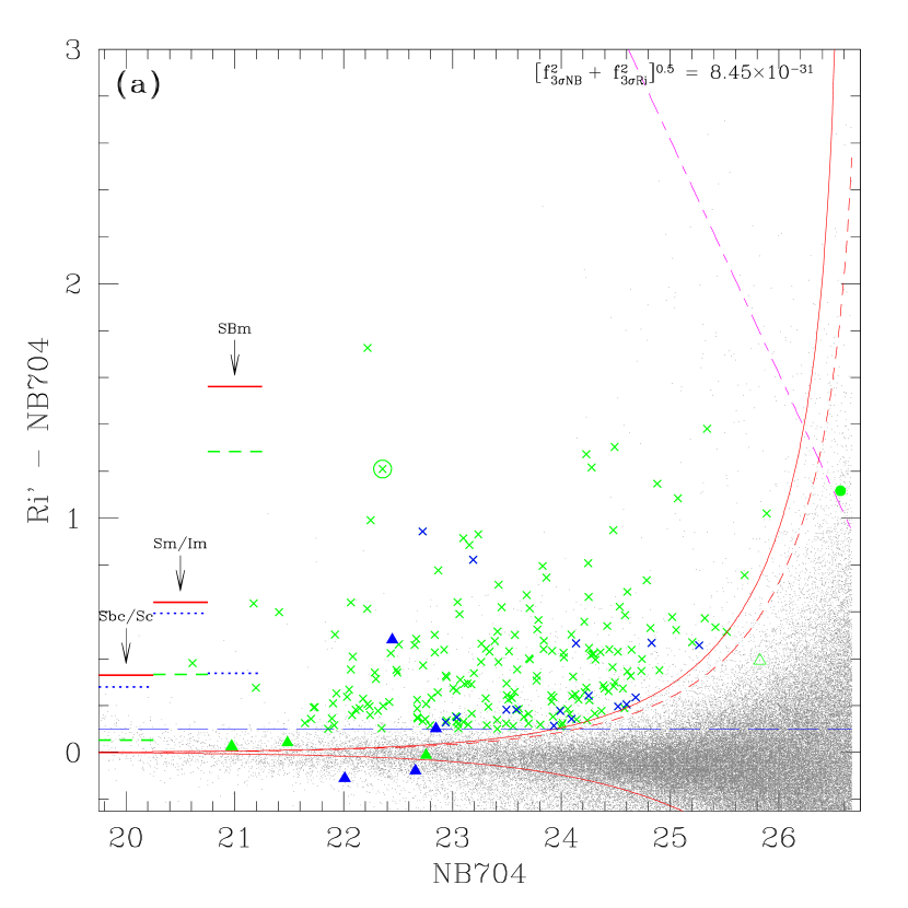
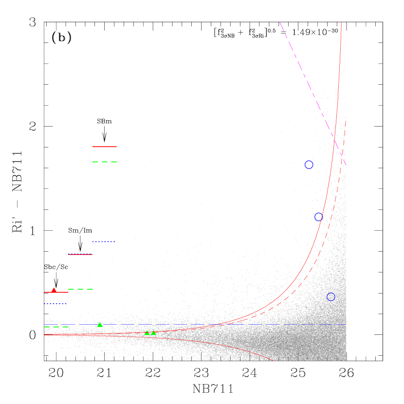
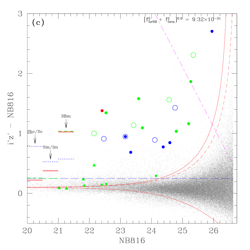
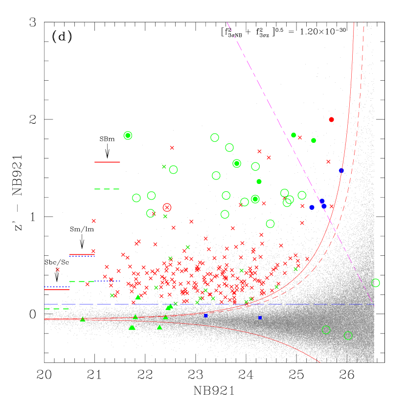
Figure 1.— NB excess plots for the (a) NB704, (b) NB711, (c) NB816, and (d) NB921 catalog. The absiccas show the NB magnitude with a 2″-aperture, and the ordinates show the line excess relative to the broad-band continuum. [O ii], [O iii]/H$\beta$, and H$\alpha$ emitters are identified as blue, green, and red, respectively in the electronic edition. Open circles are FOCAS sources, filled circles are DEIMOS targets, filled squares are serendipitous objects, crosses are NB704+921 emitters, and filled triangles are fortuitous sources. The solid and dashed lines (colored red in the electronic edition) are the excess of BB-NB for $\pm 3\sigma$ and 2.5$\sigma$, respectively. Long-dashed lines (colored blue in the electronic edition) represent an excess of (a) 0.10, (b) 0.10, (c) 0.25, and (d) 0.10 mag. Points above the short-long dashed lines (colored magenta in the electronic edition) have their broad-band continuum fainter than 3$\sigma$. Small horizontal lines on the left-hand side of the figures are the predicted excess for late type galaxies from the SDSS (Yip et al., 2004). Solid lines are for H$\alpha$, short-dashed lines are for [O iii], and dotted lines are for [O ii]. The three columns from left to right are for Sbc/Sc, Sm/Im, and SBm galaxies.

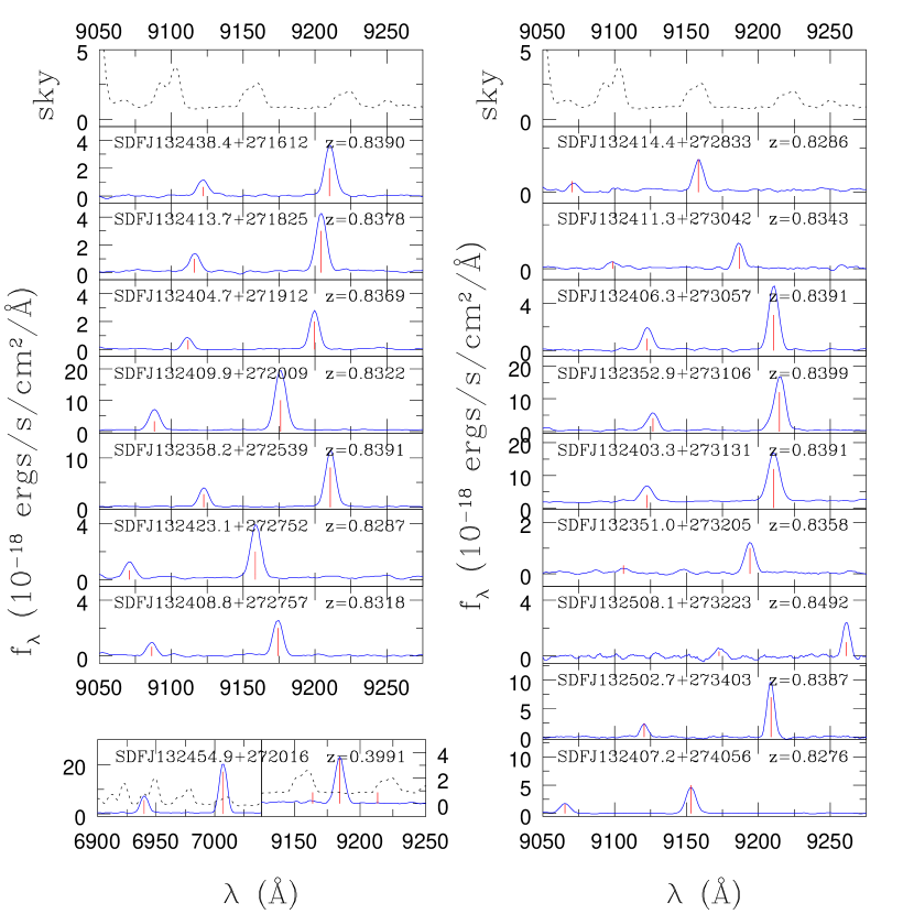
Figure 2.— Spectra of NB921 emitters from FOCAS. Vertical lines (colored red in the electronic edition) identify the location of emission lines in the spectral window. For [O iii] emitters, the lines are 4959Å and 5007Å. [O iii] lines for the H$\alpha$ emitter are shown in the adjacent panel. The lines blue-ward and red-ward of H$\alpha$ are [N ii] $\lambda\lambda$6548, 6583. The spectrum of the sky is shown in the top panels with arbitrary units and overlaid for the H$\alpha$ emitter as a dashed lines.

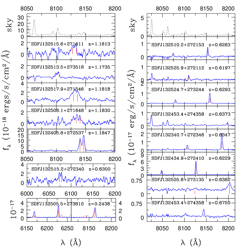
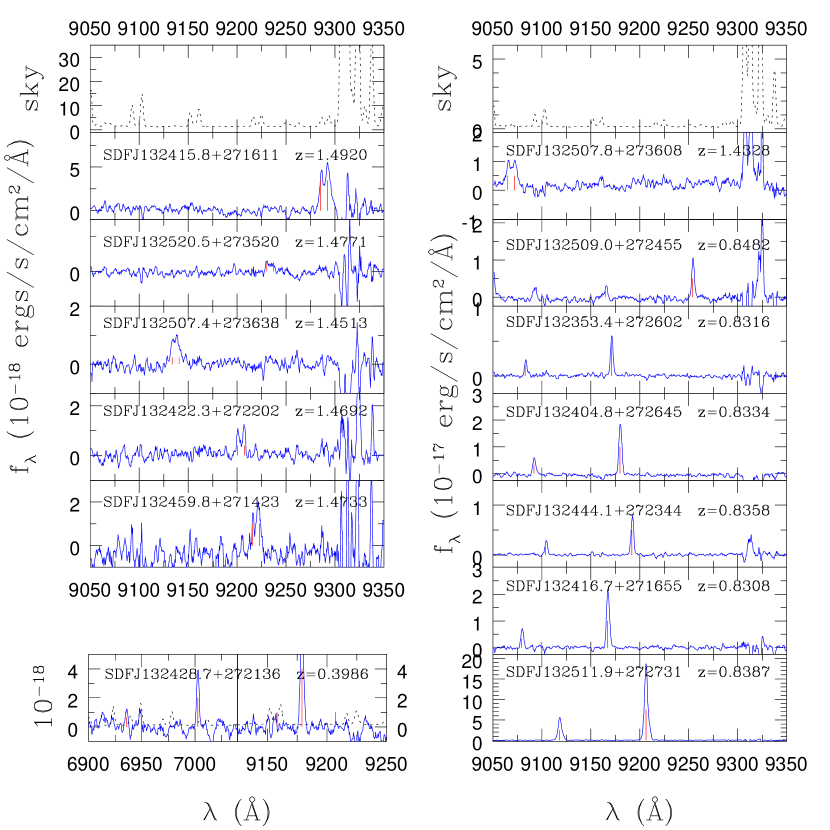
Figure 3.— DEIMOS spectra of our identified line-emitting galaxies (including serendipitous sources). NB816 emitters are shown on the left, and NB921 emitters are shown on the right. Vertical grey lines (colored red in the electronic edition) identify the location of emission lines in the spectral window. For [O ii] emitters, the lines are 3726Å and 3729Å, and 4959Å and 5007Å for [O iii]. [O iii] lines for H$\alpha$ emitters are shown in the adjacent panel. The lines blue-ward and red-ward of H$\alpha$ are [N ii] $\lambda\lambda$6548, 6583. The spectrum of the sky is shown in the top panels with units of 10^-18 and 10^-17 ergs s^-1 cm^-2 Å^-1 for [O ii] and [O iii], respectively. For H$\alpha$ emitters, the sky’s spectrum is overlaid on the source’s as a dashed line. For the $z=0.675$ galaxy at the bottom right of the left figure, the H$\beta$ line is identified in the NB816 filter.

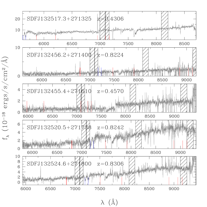
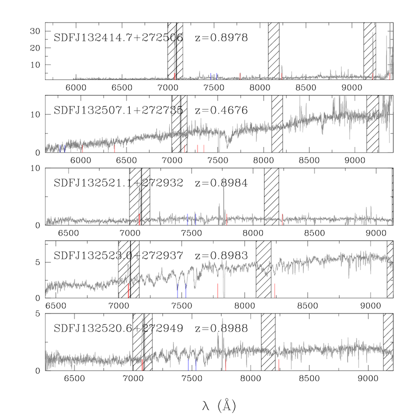
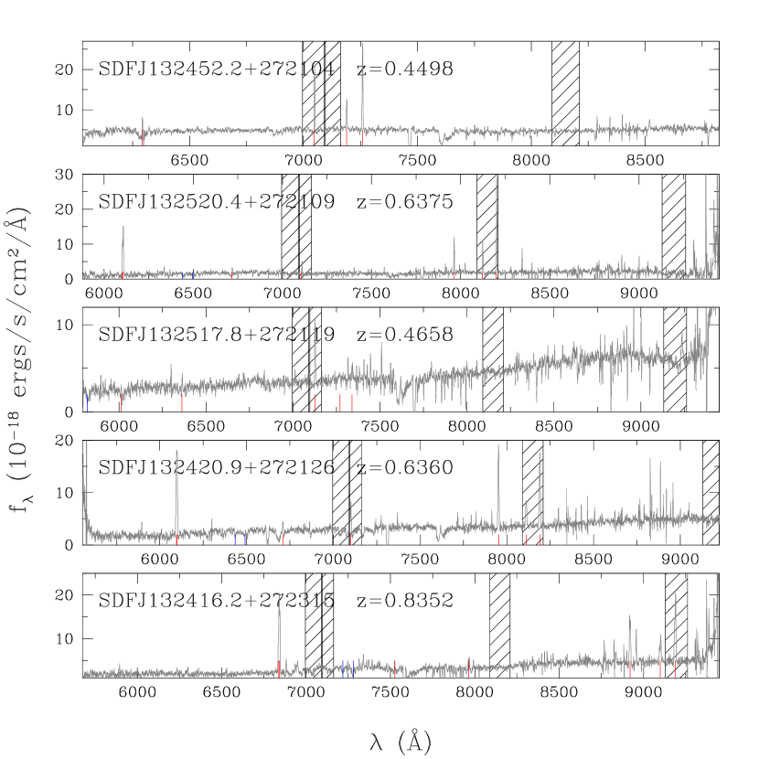
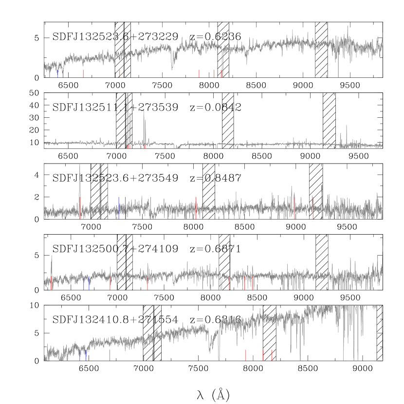
Figure 4.— Spectra of the twenty fortuitous sources. The ordinates are given in 10^-18 ergs s^-1 cm^-2 Å^-1. Vertical lines (colored red in the electronic edition) identify the location of emission lines in the spectral window. They are from short to long wavelengths: [O ii], H$\delta$, H$\gamma$, H$\beta$, [O iii] doublet, H$\alpha$, [N ii] doublet, and [S ii] doublet. The blue lines (in the electronic edition) identify the location of Ca ii K and H at 3933 and 3968Å. The FWHMs of the NB filters are shown by the shaded regions.

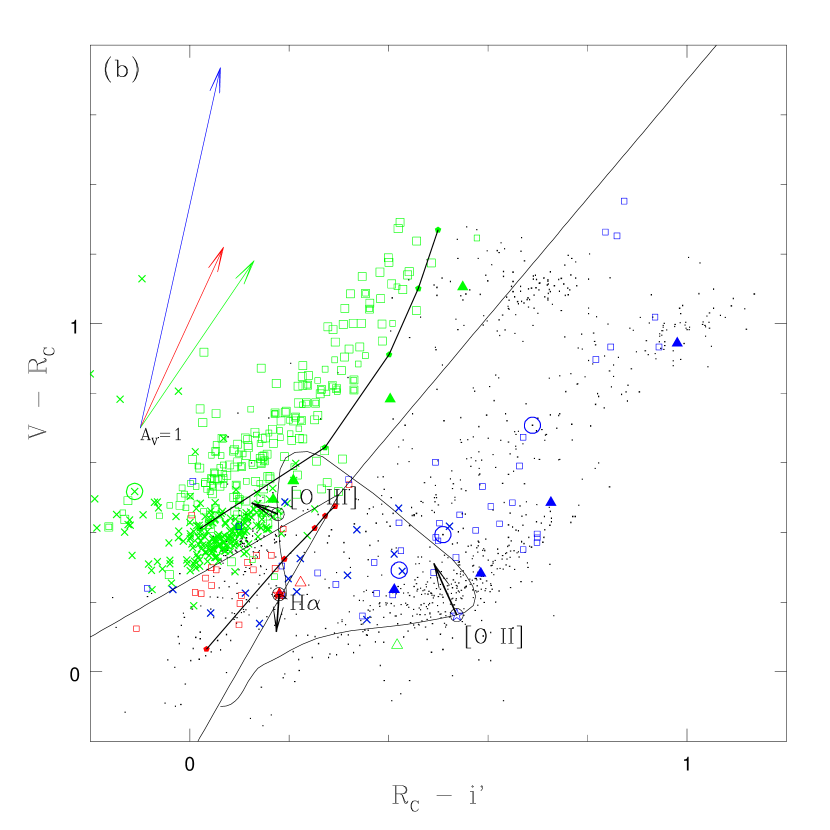
Figure 5.— Two-color diagrams in $V-R_{\rm C}$ vs. $R_{\rm C}-i\arcmin$ for (a) NB704 and (b) NB711 emitters. All spectroscopic NB704 and NB711 emitters are plotted on both diagrams. In the electronic edition, red points are H$\alpha$, blue points are [O ii], and green points are [O iii] and H$\beta$ emitters identified by FOCAS (open circles) and DEIMOS (filled circles). Open squares are galaxies from the Hawaii HDF-N, and triangles are fortuitous sources (filled) and from the NED database (open). NB704 and NB921 dual emitters are shown as crosses. The solid lines are $V-R_{\rm C}=1.70(R_{\rm C}-i\arcmin)$, $V-R_{\rm C}=0.82(R_{\rm C}-i\arcmin)+0.26$, and $V-R_{\rm C}=2.5(R_{\rm C}-i\arcmin)-0.24$. A theoretical model from Bruzual & Charlot (2003) with constant star-formation (without dust extinction) is shown by the solid black curve for $z=0$ to 1.5. Along this curve, the broad-band colors at specific redshifts of 0.07, 0.40, and 0.89 are shown by starred symbols with a circle surrounding it. Black vectors at these points indicate the direction that the colors follow with different emission line strengths. The vectors in the upper left-hand corner correspond to 1 magnitude of V extinction using the reddenning curve of Cardelli et al. (1989). Filled pentagons and thick black lines represent the colors of Yip et al. (2004)’s spectra from early to late type SDSS galaxies for $z=0.07$ and 0.40.

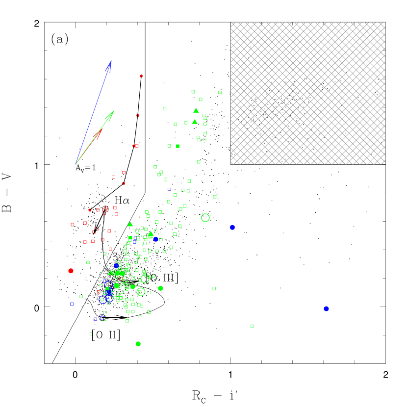
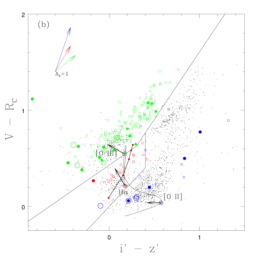
Figure 6.— Two-color diagrams in $B-V$ vs. $R_{\rm C}-i\arcmin$ (a) and $V-R_{\rm C}$ vs. $i\arcmin-z\arcmin$ (b) for NB816 emitters. In the electronic edition, red points are H$\alpha$, blue points are [O ii], and green points are [O iii] and H$\beta$ emitters identified by FOCAS (open circles) or DEIMOS (filled circles). Open squares are galaxies from the Hawaii HDF-N, filled squares are serendipitous sources, and filled triangles are fortuitous sources. The solid lines in (a) are $B-V=2.0(R_{\rm C}-i\arcmin)+0.20$ and $R_{\rm C}-i\arcmin=0.45$, and in (b) $V-R_{\rm C}=0.65(i\arcmin-z\arcmin)+0.43$, $V-R_{\rm C}=1.4(i\arcmin-z\arcmin)+0.21$, $i\arcmin-z\arcmin=0.40$, and $V-R_{\rm C}=i\arcmin-z\arcmin$. A theoretical model from Bruzual & Charlot (2003) with constant star-formation (without dust extinction) is shown by the solid black curve for $z=0$ to 1.5. Along this curve, the broad-band colors at specific redshifts of 0.24, 0.64, and 1.20 are shown by starred symbols with a circle surrounding it. Black vectors at these points indicate the direction that the colors follow with different emission line strengths. The vectors in the upper left-hand corner correspond to 1 magnitude of V extinction using the reddenning curve of Cardelli et al. (1989). Filled pentagons (red in the electronic edition) and thick black lines represent the colors of Yip et al. (2004)’s spectra from early to late for $z=0.24$.

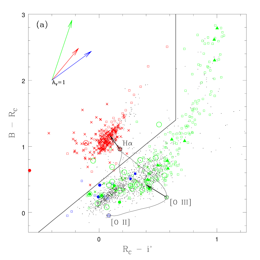
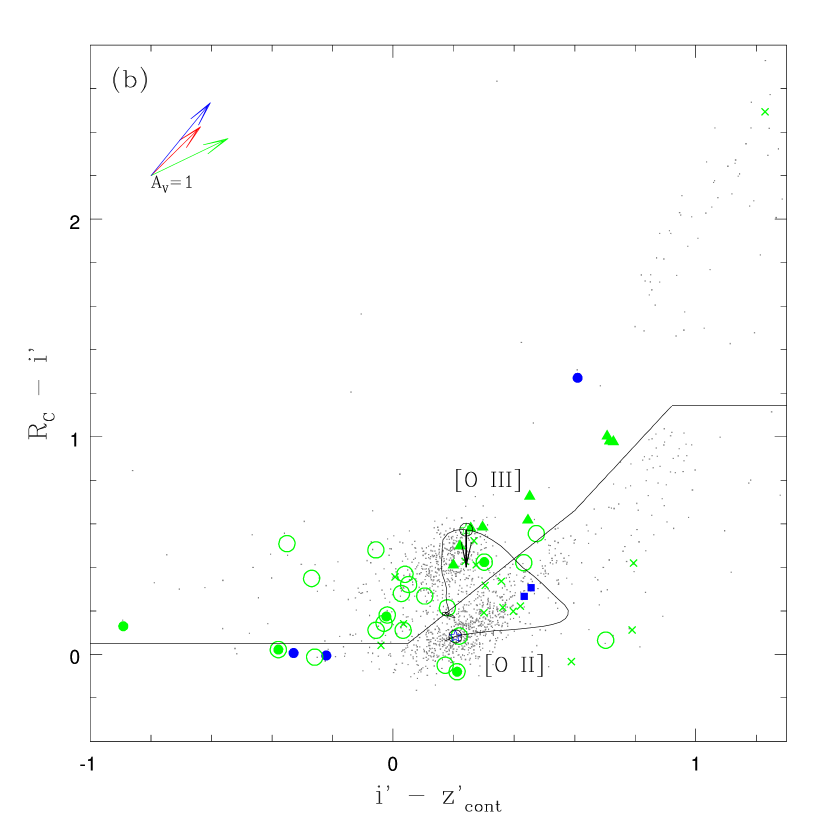
Figure 7.— Two-color diagrams in $B-R_{\rm C}$ vs. $R_{\rm C}-i\arcmin$ (a) and $R_{\rm C}-i\arcmin$ vs. $i\arcmin-z\arcmin_{\rm cont}$ (b) for NB921 emitters. In the electronic edition, red points are H$\alpha$, blue points are [O ii], and green points are [O iii] and H$\beta$ emitters identified by FOCAS (open circles) or DEIMOS (filled circles). Open squares are galaxies from the Hawaii HDF-N, filled squares are serendipitous sources, and filled triangles are fortuitous sources. NB704 and NB921 dual emitters are shown as crosses. The solid lines in (a) are $B-R_{\rm C}=1.46(R_{\rm C}-i\arcmin)+0.58$, and $R_{\rm C}-i\arcmin=0.45$, and in (b) $R_{\rm C}-i\arcmin=0.05$, $R_{\rm C}-i\arcmin=1.11(i\arcmin-z\arcmin_{\rm cont})-0.01$, $R_{\rm C}-i\arcmin=1.5(i\arcmin-z\arcmin_{\rm cont})-0.24$, and $R_{\rm C}-i\arcmin=1.14$. A theoretical model from Bruzual & Charlot (2003) with constant star-formation (without dust extinction) is shown by the solid black curve for $z=0$ to 1.5. Along this curve, the broad-band colors at specific redshifts of 0.40, 0.84, and 1.45 are shown by starred symbols with a circle surrounding it. Black vectors at these points indicate the direction that the colors follow with different emission line strengths. The vectors in the upper left-hand corner correspond to 1 magnitude of V extinction using the reddenning curve of Cardelli et al. (1989).

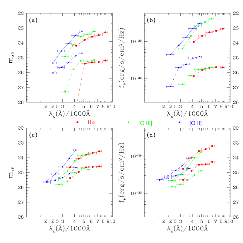
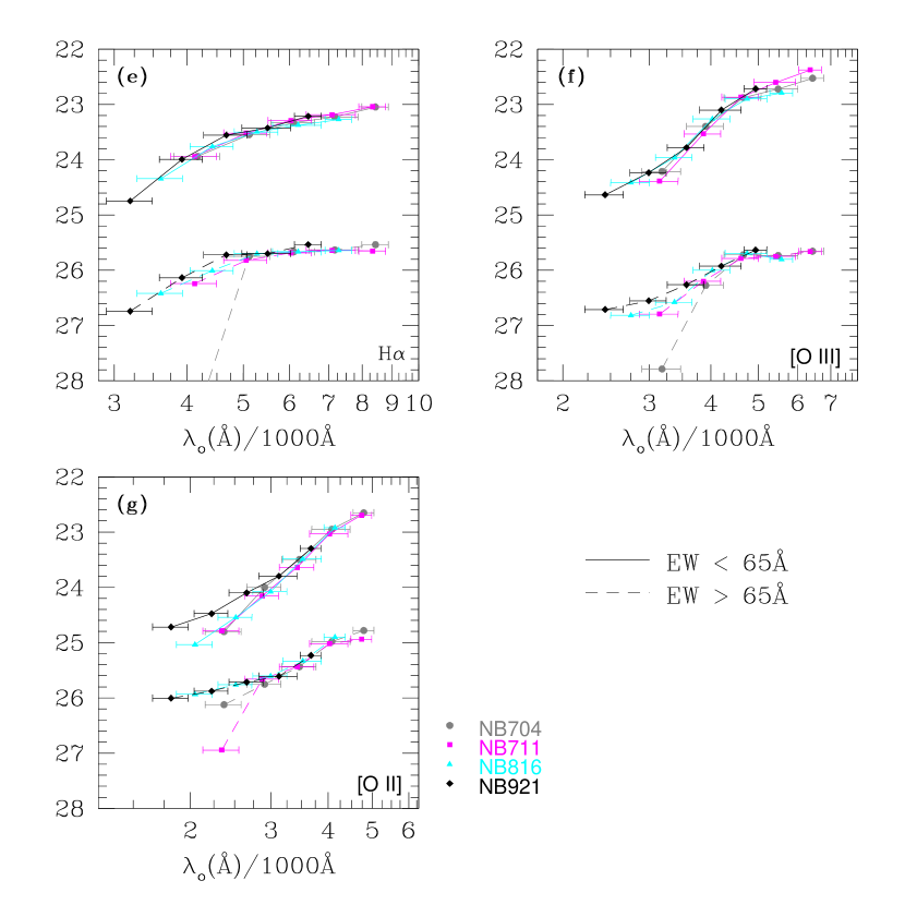
Figure 8.— Spectral energy distributions for (a) NB704, (b) NB711, (c) NB816, and (d) NB921 emitters. The outer ordinates give the AB magnitudes and the inner ones are flux densities in ergs s^-1 cm^-2 Hz^-1. The rest wavelengths of the BB filters are given on the absiccas. In the electronic edition, red, green, and blue points correspond to H$\alpha$ (circles), [O iii] (squares), and [O ii] (triangles) line emitters. The solid and dashed lines correspond to low- and high-EWs, respectively. The division is made at observed EW of 65Å. The SEDs for H$\alpha$, [O iii], and [O ii] emitters are compared in (e), (f), and (g), respectively, where vertical shifts are applied to overlap them. In (e)-(g), NB704, NB711, NB816, and NB921 emitters are given by grey circles, magenta squares, cyan triangles, and black diamonds, respectively in the electronic edition.

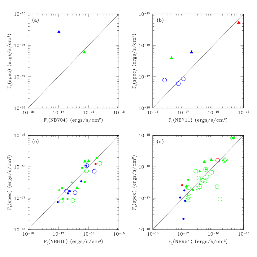
Figure 9.— Comparison between spectroscopic and photometric line fluxes for (a) NB704, (b) NB711, (c) NB816, and (d) NB921 emitters. Line fluxes are given in ergs s^-1 cm^-2. In the electronic edition, red points are H$\alpha$, blue points are [O ii], and green points are [O iii] and H$\beta$ emitters identified by FOCAS (open circles) or DEIMOS (filled circles). Filled triangles and squares are fortuitous and serendipitous sources, respectively. The solid lines represent one-to-one correspondence.

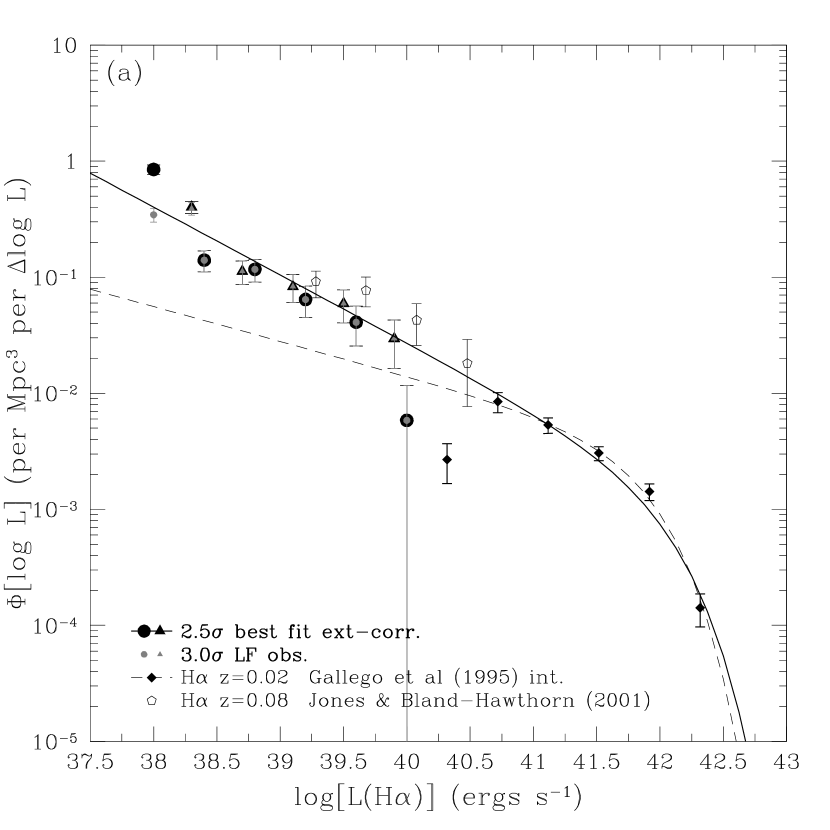
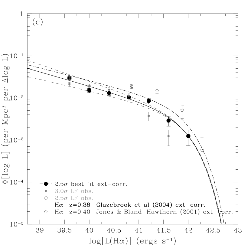
Figure 10.— The luminosity function for H$\alpha$ emitters at (a) $z=0.07-0.09$, (b) $z\approx 0.24\pm 0.01$, and (c) $z\approx 0.40\pm 0.01$. Ordinates are $\Phi[\log{L}]$ in units of Mpc${}^{-3}~{}(\Delta\log{L})^{-1}$. Absiccas are $\log{L(\rm{H}\alpha)}$ in ergs s^-1. The LFs of NB704, NB816, and NB921 are plotted as filled circles, and NB711 emitters are plotted as filled triangles in (a), where black and grey filled circles are for the $2.5\sigma$ extinction-corrected and $3\sigma$ observed sample, respectively. For NB921, the $\pm$1$\sigma$ uncertainties in $\alpha$ are shown by the two thin short-dashed black lines, and the 2.5$\sigma$ observed points are shown as open grey diamonds to illustrate the effect of incompleteness at the faint end. Open circles at the faint luminosity end are $2.5\sigma$ points excluded from the best fit given by the thick solid black lines. The luminosity functions from other studies are overlayed. Jones & Bland-Hawthorn (2001) at $z=0.08$, 0.24, and 0.40 are shown as open pentagons, Gallego et al. (1995) as short-dashed black lines with open (observed) and filled (intrinsic) diamonds, $z=0.24$ observed Hippelein et al. (2003) points are shown as open grey squares, and $z=0.2\pm 0.1$ Tresse & Maddox (1998) as filled grey diamonds and dotted line. In addition, Fujita et al. (2003) $z=0.24$ is shown as a dashed line and filled triangles (colored red in the electronic edition), Sullivan et al. (2000) as a long-dashed line (colored blue in the electronic edition) with crosses, a dot - short-dashed black line for Glazebrook et al. (2004), and Pascual et al. (2005) as open triangles. All values have been converted to the common cosmology. Extinction-corrected values follow Equation 7 with the exception of Gallego et al. (1995), Tresse & Maddox (1998), Sullivan et al. (2000), and Hippelein et al. (2003) where their extinction-corrected LF are used.

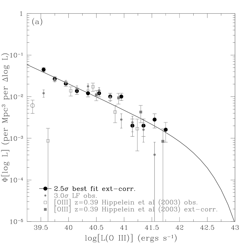
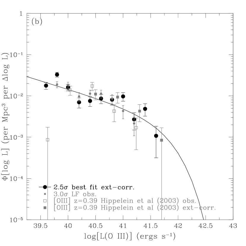
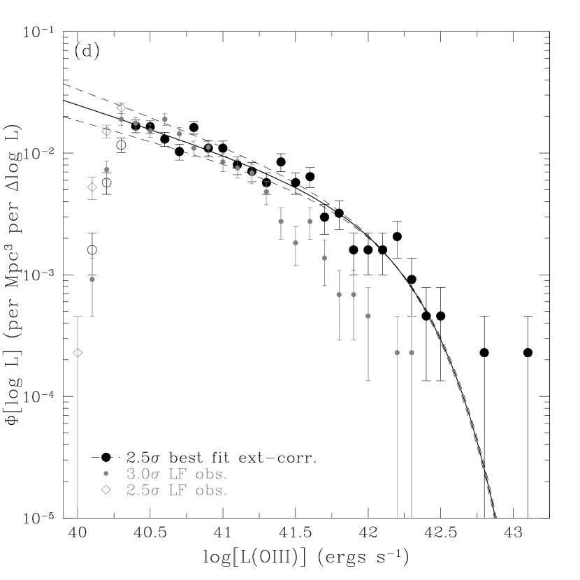
Figure 11.— The luminosity function for [O iii] emitters at (a) $z\approx 0.41\pm 0.01$, (b) $z\approx 0.42\pm 0.01$, (c) $z\approx 0.63\pm 0.01$, and (d) $z\approx 0.84\pm 0.01$. Ordinates are $\Phi[\log{L}]$ in units of Mpc${}^{-3}~{}(\Delta\log{L})^{-1}$. Absiccas are $\log{L(\textsc{O iii})}$ in ergs s^-1. The LFs of NB704, NB711, NB816, and NB921 are plotted as filled circles for the $2.5\sigma$ extinction-corrected (black) and $3\sigma$ observed (grey) sample. For NB921, the $\pm$1$\sigma$ uncertainties in $\alpha$ are shown by the two thin short-dashed black lines, and the 2.5$\sigma$ observed points are shown as open grey diamonds to illustrate the effect of incompleteness at the faint end. Open circles at the faint luminosity end are $2.5\sigma$ points excluded from the best fit given by the thick solid black lines. For NB816, the filled grey pentagons and solid line are the LF including the 192 unknown sources. The luminosity functions of Hippelein et al. (2003) at $z=0.39-0.41$ and 0.63 - 0.65 are shown as open (observed) and filled (extinction-corrected) grey squares.

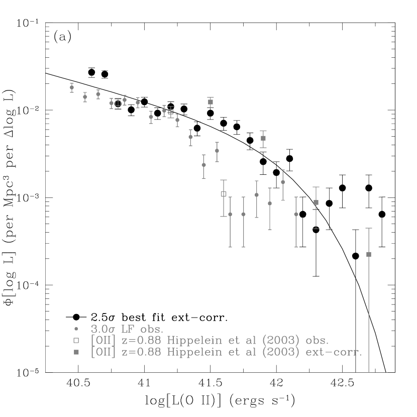
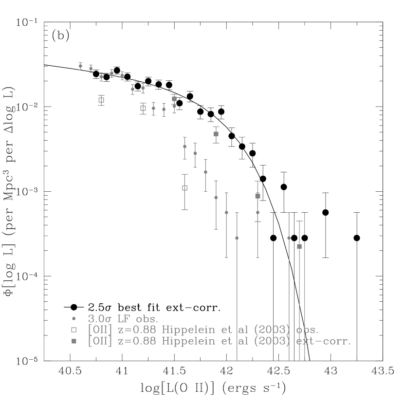
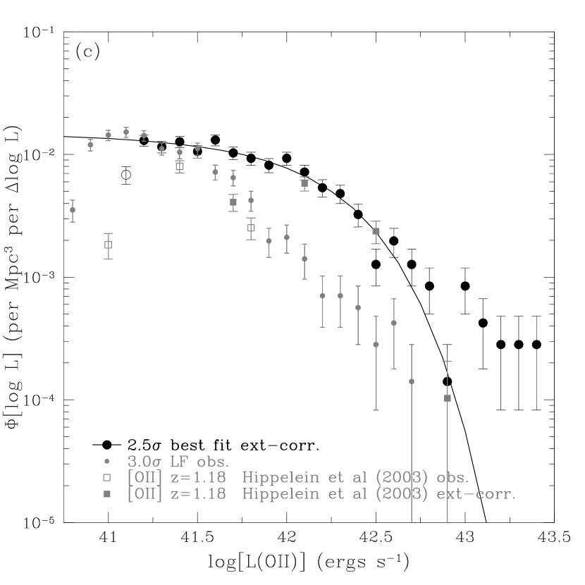
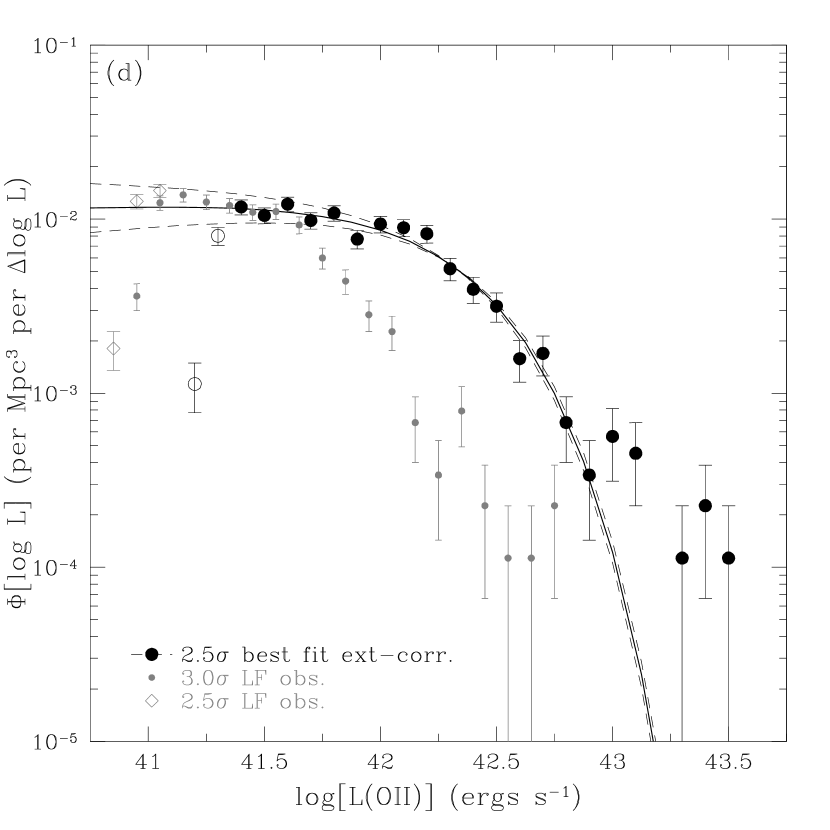
Figure 12.— The luminosity function for [O ii] emitters at (a) $z\approx 0.89\pm 0.01$, (b) $z\approx 0.91\pm 0.01$, (c) $z\approx 1.19\pm 0.02$, and (d) $z\approx 1.47\pm 0.02$. Ordinates are $\Phi[\log{L}]$ in units of Mpc${}^{-3}~{}(\Delta\log{L})^{-1}$. Absiccas are $\log{L(\textsc{O ii})}$ in ergs s^-1. The LFs for NB704, NB711, NB816, and NB921 are plotted as filled circles for the $2.5\sigma$ extinction-corrected (black) and $3\sigma$ observed (grey) sample. Open circles at the faint end are $2.5\sigma$ points excluded from the best fit given by the thick solid black lines. For NB921, the $\pm$1$\sigma$ uncertainties in $\alpha$ are shown by the two thin short-dashed black lines, and the 2.5$\sigma$ observed points are shown as open grey diamonds to illustrate the effect of incompleteness at the faint end. The luminosity functions of Hippelein et al. (2003) at $z=0.87-0.89$ and 1.18 - 1.21 are shown as open (observed) and filled (extinction-corrected) grey squares.

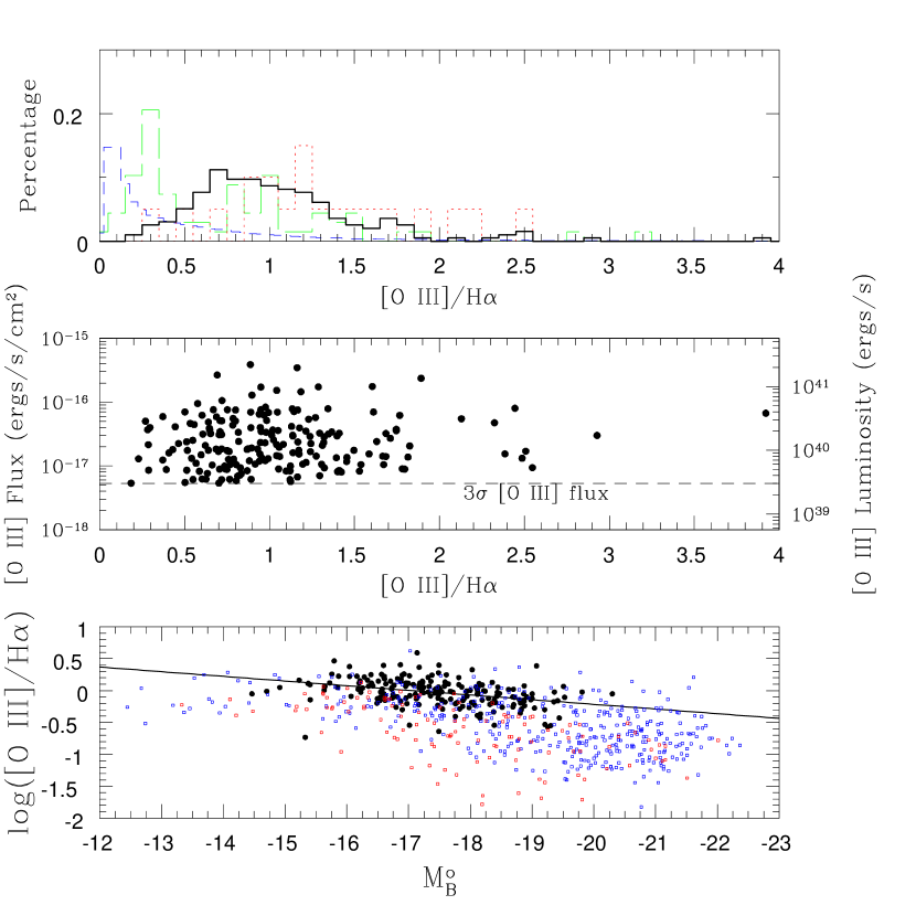
Figure 13.— [O iii]-H$\alpha$ flux ratio for NB704+921 emitters. The top diagram shows a solid black histogram for 196 $z\approx 0.40$ NB704+921 line emitters. The dotted and long-dashed histograms are from Hippelein et al. (2003) for 20 $z=0.40$ and 68 $z=0.25$ objects, respectively (colored red and green in the electronic edition). The SDSS DR2 histogram is shown as a short-dashed histogram (colored blue in the electronic edition). The middle figure shows the [O iii] flux and luminosity as a function of the ratio. The bottom figure shows the logarithm of the ratio as a function of $M_{B}^{o}$. In the electronic edition, the red and blue open squares are nearby star-forming galaxies from Jansen et al. (2000) and Moustakas & Kennicutt (2006), respectively. The best fit to the black points is given in Equation 11.

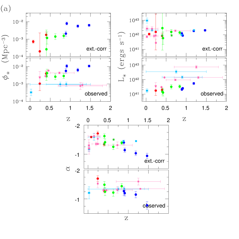
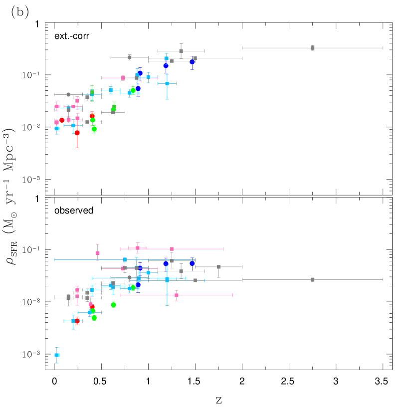
Figure 14.— Schechter LF parameters and SFR density as a function of redshift. NB emitters are shown as circles and squares represent previous emission line surveys: [O ii] (light blue in the electronic edition) values are from Hammer et al. (1997), Hogg et al. (1998), Sullivan et al. (2000), Gallego et al. (2002), Hicks et al. (2002), and Teplitz et al. (2003). H$\alpha$ (pink in the electronic edition) points are from Gallego et al. (1995), Tresse & Maddox (1998), Glazebrook et al. (1999), Yan et al. (1999), Hopkins et al. (2000), Moorwood et al. (2000), Sullivan et al. (2000), Tresse et al. (2002), Fujita et al. (2003), Pérez-González et al. (2003), Glazebrook et al. (2004), and Pascual et al. (2005). [O ii], [O iii] (dark green in electronic edition), and H$\alpha$ data from Hippelein et al. (2003) are also included. Grey points are UV measurements from Cowie et al. (1999), Sullivan et al. (2000), Massarotti et al. (2001), and Wilson et al. (2002).

Figure 15.— $B-R_{\rm C}$ and $R_{\rm C}-I_{\rm C}$ colors for Hawaii HDF-N galaxies with NB816 redshifts. Filled circles are H$\alpha$ ($z\approx 0.24$), open triangles are [O iii] or H$\beta$ ($z\approx 0.63$), and [O ii] are shown as open squares. The solid line is the selection criterion of Fujita et al. (2003): $B-R_{\rm C}=2(R_{\rm C}-I_{\rm C})+0.20$.

References

- Aragón-Salamanca et al. (2003) Aragón-Salamanca, A., Alonso-Herrero, A., Gallego, J., García-Dabó, C. E., Pérez-González, P. G., Zamorano, J., & Gil de Paz, A. 2003, ASP Conf. Ser. 297: Star Formation Through Time, 297, 191
- Ajiki et al. (2003) Ajiki, M., et al. 2003, AJ, 126, 2091
- Ajiki et al. (2006) Ajiki, M., et al. 2006, PASJ, 58, 113
- Arnouts et al. (2005) Arnouts, S., et al. 2005, ApJ, 619, L43
- Bertin & Arnouts (1996) Bertin, E., & Arnouts, S. 1996, A&AS, 117, 393
- Brinchmann et al. (2004) Brinchmann, J., Charlot, S., White, S. D. M., Tremonti, C., Kauffmann, G., Heckman, T., & Brinkmann, J. 2004, MNRAS, 351, 1151
- Bruzual & Charlot (2003) Bruzual, G., & Charlot, S. 2003, MNRAS, 344, 1000
- Capak et al. (2004) Capak, P., et al. 2004, AJ, 127, 180
- Cardelli et al. (1989) Cardelli, J. A., Clayton, G. C., & Mathis, J. S. 1989, ApJ, 345, 245
- Connolly et al. (1997) Connolly, A. J., Szalay, A. S., Dickinson, M., Subbarao, M. U., & Brunner, R. J. 1997, ApJ, 486, L11
- Cowie et al. (1999) Cowie, L. L., Songaila, A., & Barger, A. J. 1999, AJ, 118, 603
- Cowie et al. (2004) Cowie, L. L., Barger, A. J., Hu, E. M., Capak, P., & Songaila, A. 2004, AJ, 127, 3137
- Doherty et al. (2006) Doherty, M., Bunker, A., Sharp, R., Dalton, G., Parry, I., & Lewis, I. 2006, MNRAS, 370, 331
- Drozdovsky et al. (2005) Drozdovsky, I., Yan, L., Chen, H.-W., Stern, D., Kennicutt, R. J., Spinrad, H., & Dawson, S. 2005, AJ, 130, 1324
- Faber et al. (2003) Faber, S. M., et al. 2003, Proc. SPIE, 4841, 1657
- Fujita et al. (2003) Fujita, S. S., et al. 2003, ApJ, 586, L115
- Gabasch et al. (2004) Gabasch, A., et al. 2004, A&A, 421, 41
- Gabasch et al. (2006) Gabasch, A., et al. 2006, A&A, 448, 101
- Gallego et al. (1995) Gallego, J., Zamorano, J., Aragon-Salamanca, A., & Rego, M. 1995, ApJ, 455, L1
- Gallego et al. (1997) Gallego, J., Zamorano, J., Rego, M., & Vitores, A. G. 1997, ApJ, 475, 502
- Gallego et al. (2002) Gallego, J., García-Dabó, C. E., Zamorano, J., Aragón-Salamanca, A., & Rego, M. 2002, ApJ, 570, L1
- Glazebrook et al. (1999) Glazebrook, K., Blake, C., Economou, F., Lilly, S., & Colless, M. 1999, MNRAS, 306, 843
- Glazebrook et al. (2004) Glazebrook, K., Tober, J., Thomson, S., Bland-Hawthorn, J., & Abraham, R. 2004, AJ, 128, 2652
- Hammer et al. (1997) Hammer, F., et al. 1997, ApJ, 481, 49
- Hicks et al. (2002) Hicks, E. K. S., Malkan, M. A., Teplitz, H. I., McCarthy, P. J., & Yan, L. 2002, ApJ, 581, 205
- Hippelein et al. (2003) Hippelein, H., et al. 2003, A&A, 402, 65
- Hogg et al. (1998) Hogg, D. W., Cohen, J. G., Blandford, R., & Pahre, M. A. 1998, ApJ, 504, 622
- Hopkins et al. (2000) Hopkins, A. M., Connolly, A. J., & Szalay, A. S. 2000, AJ, 120, 2843
- Hopkins et al. (2001) Hopkins, A. M., Connolly, A. J., Haarsma, D. B., & Cram, L. E. 2001, AJ, 122, 288
- Hopkins (2004) Hopkins, A. M. 2004, ApJ, 615, 209
- Hu et al. (2002) Hu, E. M., Cowie, L. L., McMahon, R. G., Capak, P., Iwamuro, F., Kneib, J.-P., Maihara, T., & Motohara, K. 2002, ApJ, 568, L75
- Hu et al. (2004) Hu, E. M., Cowie, L. L., Capak, P., McMahon, R. G., Hayashino, T., & Komiyama, Y. 2004, AJ, 127, 563
- Iwamuro et al. (2000) Iwamuro, F., et al. 2000, PASJ, 52, 73
- Iye et al. (2004) Iye, M., et al. 2004, PASJ, 56, 381
- Jansen et al. (2000) Jansen, R. A., Fabricant, D., Franx, M., & Caldwell, N. 2000, ApJS, 126, 331
- Jansen et al. (2001) Jansen, R. A., Franx, M., & Fabricant, D. 2001, ApJ, 551, 825
- Jones & Bland-Hawthorn (2001) Jones, D. H., & Bland-Hawthorn, J. 2001, ApJ, 550, 593
- Kaifu (1998) Kaifu, N. 1998, Proc. SPIE, 3352, 14
- Kashikawa et al. (2002) Kashikawa, N., et al. 2002, PASJ, 54, 819
- Kashikawa et al. (2004) Kashikawa, N., et al. 2004, PASJ, 56, 1011
- Kashikawa et al. (2006) Kashikawa, N., et al. 2006, ApJ, 648, 7
- Kennicutt (1983) Kennicutt, R. C. 1983, ApJ, 272, 54
- Kennicutt (1992) Kennicutt, R. C. 1992, ApJ, 388, 310
- Kennicutt (1998) Kennicutt, R. C. 1998, ARA&A, 36, 189
- Kewley, Gellar, & Jansen (2004) Kewley, L. J., Geller, M. J., & Jansen, R. A. 2004, AJ, 127, 2002
- Kobulnicky et al. (1999) Kobulnicky, H. A., Kennicutt, R. C., & Pizagno, J. L. 1999, ApJ, 514, 544
- Kodaira et al. (2003) Kodaira, K., et al. 2003, PASJ, 55, L17
- Kodama et al. (2004) Kodama, T., Balogh, M. L., Smail, I., Bower, R. G., & Nakata, F. 2004, MNRAS, 354, 1103
- Lilly et al. (1996) Lilly, S. J., Le Fevre, O., Hammer, F., & Crampton, D. 1996, ApJ, 460, L1
- Malkan et al. (1995) Malkan, M., Teplitz, H., & McLean, I. 1995, ApJ, 448, L5
- Massarotti et al. (2001) Massarotti, M., Iovino, A., & Buzzoni, A. 2001, ApJ, 559, L105
- Meisenheimer & Wolf (2002) Meisenheimer, K., & Wolf, C. 2002, Astronomy and Geophysics, 43, 15
- McCarthy et al. (1999) McCarthy, P. J., et al. 1999, ApJ, 520, 548
- Moorwood et al. (2000) Moorwood, A. F. M., van der Werf, P. P., Cuby, J. G., & Oliva, E. 2000, A&A, 362, 9
- Moustakas & Kennicutt (2006) Moustakas, J., & Kennicutt, R. C., Jr. 2006, ApJS, 164, 81
- Oke (1990) Oke, J. B. 1990, AJ, 99, 1621
- Oke et al. (1995) Oke, J. B., et al. 1995, PASP, 107, 375
- Osterbrock (1989) Osterbrock, D. E. 1989, Astrophysics of Gaseous Nebulae and Active Galactic Nuclei (Mill Valley, CA: University Science Books)
- Ouchi et al. (2003) Ouchi, M., et al. 2003, ApJ, 582, 60
- Pascual et al. (2005) Pascual, S., Villar, V., Gallego, J., Zamorano, J., Pelló, R., Díaz, C., & Aragón-Salamanca, A. 2005, Revista Mexicana de Astronomia y Astrofisica Conference Series, 24, 268