Long-term monitoring of the X-ray afterglow of GRB 050408 with Swift/XRT

We present observations of the X-ray afterglow of GRB 050408, a gamma-ray burst discovered by HETE-II. Swift began observing the field 42 min after the burst, performing follow-up over a period of 38 d (thus spanning three decades in time). The X-ray light curve showed a steepening with time, similar to many other afterglows. However, the steepening was unusually smooth, over the duration of the XRT observation, with no clear break time. The early decay was too flat to be described in terms of standard models. We therefore explore alternative explanations, such as the presence of a structured afterglow or of long-lasting energy injection into the fireball from the central GRB engine. The lack of a sharp break puts constraints on these two models. In the former case, it may indicate that the angular energy profile of the jet was not a simple power law, while in the second model it implies that injection did not stop abruptly. The late decay may be due either to a standard afterglow (that is, with no energy injection), or to a jetted outflow still being refreshed. A significant amount of absorption was present in the X-ray spectrum, corresponding to a rest-frame Hydrogen column density $N_{\rm H}=1.2_{-0.3}^{+0.4}\times 10^{22}$ cm^-2, indicative of a dense environment.

1 Introduction

The Swift Gamma-Ray Burst Explorer (Gehrels et al. 2004), designed to study gamma-ray bursts (GRBs), has unique characteristics allowing the prompt observation of GRB afterglows (see Barthelmy et al. 2005; Burrows et al. 2005; Roming et al. 2005, for a description of the Swift instruments). This has opened up the opportunity to study the previously unexplored early phases of their evolution.

On the other hand, being fully devoted to GRB studies, Swift also has the capability to perform detailed, long-term monitoring of afterglows. To date, a number of GRBs have been observed up to $\sim 1$ month after the explosion (e.g. XRF 050416A; Mangano et al. 2006), allowing a systematic study of the late phases of their evolution. Swifts rapid slewing capabilities also allows the prompt follow-up to alerts coming from other satellites, such as HETE-II and INTEGRAL. GRB 050408 was the first burst observed by Swift which was not autonomously-triggered by the Burst Alert Telescope (BAT) barthelmy onboard.

GRB 050408 was detected by HETE-II at 16:22:50.93 UT on 2005 April 8 and localized by the Soft X-ray Camera (SXC) at RA(J2000)$\mbox{}=12^{\mathrm{h}}02^{\mathrm{m}}15^{\mathrm{s}}$, Dec(J2000)$\mbox{}=10\degr 52\arcmin 01\arcsec$ (80″ error radius, 90% containment; Sakamoto et al. 2005). The burst duration was $T_{90}\sim 34$ s in the 7–40 and 7–80 keV bands, and $T_{90}\sim 15$ s in the 30–400 keV band. Spectral analysis of the prompt emission showed that the fluence was $\sim 1.4\times 10^{-6}$ erg cm^-2 and $\sim 1.9\times 10^{-6}$ erg cm^-2 in the 2–30 keV and 30–400 keV energy bands, respectively. Using the classification defined by Lamb et al. (2005), GRB 050408 can therefore be classified as an “X-ray rich” GRB (Sakamoto et al. 2005).

On the basis of the HETE-II position, reported soon after the discovery via a GCN notice, a target of opportunity (TOO) was uploaded to Swift and the NFIs were pointed at the target about 42 min after the trigger. The Swift XRT detected an uncatalogued, fading source inside the SXC error box (Wells et al. 2005), which was later refined with an error circle of 5″ radius (Chincarini et al. 2005). Following the initial observation, XRT continued monitoring the afterglow for several weeks, leading to a long, well-sampled light curve.

Several follow-up observations were performed at other wavelengths. An optical counterpart was discovered inside the SXC error circle (de Ugarte Postigo et al. 2005), using the 1m and 6m telescopes at the Special Astrophysical Observatory. This object was later seen to fade, confirming its afterglow nature (Huang et al. 2005). The astrometric position was provided by Chen et al. (2005), who located the source at the coordinates RA(J2000)$\mbox{}=12^{\mathrm{h}}02^{\mathrm{m}}17\aas@@fstack{s}328$, Dec(J2000)$\mbox{}=+10\degr 51\arcmin 09\aas@@fstack{\prime\prime}47$ (0$\aas@@fstack{\prime\prime}$25 error radius). A spectrum of the optical afterglow obtained with the LDSS-3 instrument on the Magellan/Clay telescope showed the presence of emission and absorption lines at a redshift $z=1.236$ (Berger et al. 2005a, b). The Gemini telescope found a consistent value of $z=1.2357\pm 0.0002$ (Prochaska et al. 2005; Foley et al. 2006). Many other optical telescopes, including the 3.6m Telescopio Nazionale Galileo (TNG), detected and monitored the optical afterglow. The analysis of the TNG data, taken simultaneously with the XRT observation, is presented in a separate paper (Covino et al. 2006). Some of the afterglow properties have been discussed by Foley et al. (2006). At the location of the afterglow, UVOT detected a faint, low-significance source in the coadded $U$-band image (Holland et al. 2005). No detection was possible in the other optical and ultraviolet filters. Very Large Array radio observations at 8.5 GHz revealed no sources at the afterglow position, down to a 2-$\sigma$ upper limit of 74 $\mu$Jy on 2005 Apr 9.26 UT (Soderberg 2005).

In the following sections we report a detailed analysis of the XRT follow-up observations. In Sect. 2 we describe the XRT data reduction and analysis, and in Sect. 3 we discuss the results. A summary of our work is reported in Sect. 4. Throughout the work, we follow the notation $F_{\nu}(t,\nu)\propto t^{-\alpha}\nu^{-\beta}$ for the time and spectral dependency of the flux. The times quoted are with respect to the HETE-II trigger time.

Table 1: X-ray afterglow light curve. The first column reports the center of the time bin, expressed in seconds since trigger.

Time	Bin size	Count rate
(s)	(s)	(10-2 count s-1)
2612	120	23$\pm$5
2732	120	30$\pm$5
2852	120	29$\pm$5
6302	500	19$\pm$3
6802	500	15$\pm$2
7302	500	16.6$\pm$1.8
7802	500	13.0$\pm$2.0
8302	500	14.8$\pm$1.7
13302	500	9.7$\pm$1.5
13802	500	10.8$\pm$1.5
14302	500	8.8$\pm$1.4
19202	900	6.1$\pm$1.2
20102	900	6.7$\pm$1.0
25052	1000	6.0$\pm$1.2
26052	1000	5.0$\pm$1.0
30482	2660	3.5$\pm$0.7
40002	10700	2.7$\pm$0.6
50702	10700	3.1$\pm$0.6
61402	10700	2.7 $\pm$0.5
281121	52356	0.53$\pm$0.12
418938	80974	0.47$\pm$0.13
618410	100110	0.24$\pm$0.05
1492073	353910	0.044$\pm$0.010
1842640	173812	0.050$\pm$0.010
2476438	225974	0.035$\pm$0.012

2 XRT data analysis

XRT observations of the GRB 050408 field started on 2005 April 8 at 17:05:17 UT (2545 s after the HETE-II trigger); data collection in photon counting (PC) mode started a few seconds later (see Hill et al. (2004) and Hill et al. (2005) for a description of XRT readout modes). Swift subsequently continued monitoring the GRB field at later times, collecting a total of 12 observations over a period of 38 d. The total exposure time in PC mode was $\sim 223$ ks. Occasionally, due to the high background, the XRT switched into windowed timing mode. However, the source count rate was very low in these frames, and therefore these data were not included in our analysis.

The XRT data from the SDC archive at the NASA Goddard Space Flight Center were processed with the XRTDAS software package (v. 1.7.1) developed at the ASI Science Data Center. Calibrated and cleaned level-2 event files were produced with the xrtpipeline task, applying the standard screening criteria: frames with a CCD temperature greater than $-47$ ^∘C were rejected, and bad pixels and bad aspect time intervals were eliminated.

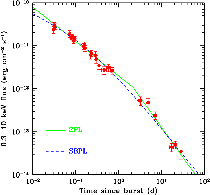
Figure 1: The 0.3–10 keV X-ray light curve of the afterglow of GRB 050408 (PC mode data only). The solid and dashed lines show the best-fit models assuming a sharply- (2PL) and smoothly- (SBPL) broken power law, respectively.

Table 2: Best-fit parameters with their associated 68% confidence intervals, for different functional forms: single power law (PL), sharply broken power law (2PL), smoothly broken power law (SBPL), and Beuermann fit (B; Beuermann et al. 1999) for two values of the smoothness parameter $s$.

Model	$\chi^{2}_{\rm r}$ (dof)	$\alpha_{1}$		$\alpha_{2}$		$t_{\rm b}$ (d)
		Best	68% C.I.	Best	68% C.I.	Best	68% C.I.
PL	2.50 (23)	0.99	$0.97<\alpha_{1}<1.01$	—	—	—	—
2PL	1.0 (21)	0.80	$0.49<\alpha_{1}<0.67,0.76<\alpha_{1}<0.84$	1.40	$1.25<\alpha_{2}<1.55$	2.2	$0.12<t_{\rm b}<0.18,1.3<t_{\rm b}<3.0$
SBPL	0.92 (21)	0.46	$-0.12<\alpha_{1}<0.78$	1.24	$1.11<\alpha_{2}<1.91$	$0.21$	$0.05<t_{\rm b}<6.6$
B, $s=0.1$	0.89 (21)	0.21	$\alpha_{1}<0.31$	2.05	$1.81<\alpha_{2}<2.89$	unconstrained
B, $s=0.5$	0.89 (21)	0.13	$\alpha_{1}<0.75$	1.51	$1.15<\alpha_{2}<3.10$	unconstrained

2.1 Image analysis

The 0.3–10 keV PC mode image of the field was analyzed with the XIMAGE package (v. 4.3). A previously uncatalogued, bright X-ray source was clearly detected inside the HETE-II error circle, at the coordinates RA(J2000)$\mbox{}=12^{\mathrm{h}}02^{\mathrm{m}}17\aas@@fstack{s}29$, Dec(J2000)$\mbox{}=10\degr 51\arcmin 11\aas@@fstack{\prime\prime}4$ (3$\aas@@fstack{\prime\prime}$5 error radius; 90% containment). This position and its error were evaluated taking into account the latest XRT boresight calibration (Moretti et al. 2006). The XRT coordinates are 60″ and 1$\aas@@fstack{\prime\prime}$95 away from the HETE-II error box center and the optical afterglow position, respectively. Another non-fading source with count rate $(2.9\pm 0.1)\times 10^{-3}$ count s^-1 is present inside the HETE-II error circle, at a distance of $\approx 38\arcsec$ from the afterglow. To avoid contamination from this source, the events for the temporal and spectral analysis were selected from a circular region of 8 pixels (19″) radius centered at the afterglow position, which contains about 77% of the photons at 1.5 keV (Moretti et al. 2005). The appropriate ancillary response file was used to correct for the PSF losses.

2.2 Temporal analysis

For the temporal analysis, the standard grade selection for PC mode (grades from 0 to 12) was adopted, in order to maximize the statistics. Only the 0.3–10 keV energy range was considered. The background in the extraction region was evaluated by comparing several source-free boxes in the field and, since it was stable during the whole observation, a constant level of $1.3\times 10^{-4}$ count s^-1 was subtracted from the light curve. Moreover, the contribution of the nearby serendipitous source was evaluated computing the number of photons falling inside the afterglow extraction region and the afterglow count rate was corrected for this contamination. The light curve was binned to ensure a minimum of 20 counts per bin. The data are reported in Table  1. The count rate was converted to an unabsorbed 0.3–10 keV flux using a conversion factor of $1.0\times 10^{-10}$ erg cm^-2 count^-1, obtained using the results from the spectral analysis (Sect 2.3). The light curve is shown in Fig. 1 (points). A gap of approximately two days is present in the data due to the close proximity of the Moon preventing the NFIs from observing.

We initially fit the afterglow decay with a single power law, obtaining an unacceptable $\chi^{2}_{\rm r}=2.5$ (23 degrees of freedom, d.o.f.). Looking at the residuals, a systematic deviation of the data from the model was apparent, showing a continuous steepening of the light curve with time. We thus fitted the data with a broken power law ($F\propto t^{-\alpha_{1}}$ for $t<t_{\rm b}$, $F\propto t^{-\alpha_{2}}$ for $t>t_{\rm b}$), where $\alpha_{1}$ and $\alpha_{2}$ are the early- and late-time decay slopes, respectively, and $t_{\rm b}$ is the break time. The best fit (Fig. 1, solid line) significantly improved, yielding $\chi^{2}_{\rm r}=1.0$ for 21 d.o.f. (null hypothesis probability of $6.6\times 10^{-5}$, according to an $F$-test). The best fit parameters, together with their confidence intervals, are reported in Table 2. Errors were computed leaving all parameters free to vary. The fit, and in particular $t_{\rm b}$, is not well constrained. Fig. 2 (upper panel) shows the behaviour of $\chi^{2}_{\rm r}$ as a function of $t_{\rm b}$. Two minima are apparent at approximately the same level (with the larger value of $t_{\rm b}$ being slightly preferred). In an independent analysis, Foley et al. (2006) indicated the lower value as the best fit. The reason for the discrepancy is possibly due to minor differences in the reduction process (e.g. background subtraction, data binning). However, our results are consistent with those derived by Chincarini et al. (2006) and Nousek et al. (2006) (who analyzed only the first part of the light curve). The smoothness of the light curve prompted us to attempt different functional forms, using the so-called smoothly-broken power law (SBPL) model: $F(t)\propto 1/[(t/t_{\rm b})^{\alpha_{1}}+(t/t_{\rm b})^{\alpha_{2}}]$. This provided a slightly better fit ($\chi^{2}_{\rm r}=0.92$ for 21 d.o.f.; dashed line in Fig. 1), but $t_{\rm b}$ could not be constrained (Fig. 2, middle panel). Similarly, $t_{\rm b}$ could not be constrained with a fit to the Beuermann model ($F(t)\propto[(t/t_{\rm b})^{s\alpha_{1}}+(t/t_{\rm b})^{s\alpha_{2}}]^{-1/s}$; Beuermann et al. 1999). The parameter $s$ (the smoothness index) controls how fast the transition between the two phases happens: large values of $s$ imply a sharp break. Leaving all parameters free, small values of $s$ (i.e., a smooth break) were systematically preferred ($s=0.1$–0.5) but the fit did not converge. Fixing $s$ to a set of definite values allowed the confidence intervals for the parameters to be determined (Fig. 2, lower panel).

Finally, in consideration of the fact that the values of the last three data points of the light curve are consistent within the errors, we checked for the presence of a persistent X-ray emission coming from the afterglow host. We found that adding a constant component to the broken power law model (2PL) does not yield a significant improvement to the fit ($F$-test probability of a chance improvement $\sim 80\%$).

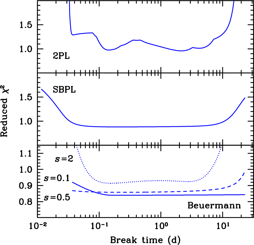
Figure 2: Reduced $\chi^{2}$ as a function of the break time $t_{\rm b}$ for three functional forms: from top to bottom, joint broken power law (2PL), smoothly broken power law (SBPL), and the Beuermann fit, for different values of the smoothness parameter $s$ (Beuermann et al. 1999).

Table 3: Results of the spectral fits to the X-ray afterglow of GRB 050408. An asterisk indicates a frozen parameter. The redshifts for the Galactic and host absorption were kept fixed at $z=0$ and $z=1.2357$, respectively. The errors are at 90% confidence level for one interesting parameter.

	Galactic absorption			Galactic + host absorption
Time range	$\beta$	$N_{\rm H}$	$\chi^{2}_{\rm r}$ (d.o.f.)	$\beta$	Galactic $N_{\rm H}$	Host $N_{\rm H}$	$\chi^{2}_{\rm r}$ (d.o.f.)
		$10^{21}$ cm-2			$10^{21}$ cm-2	$10^{21}$ cm-2
All data	$1.3\pm 0.2$	$2.9\pm 0.6$	1.4 (39)	$1.1\pm 0.1$	$0.174^{*}$	$12^{+4}_{-3}$	1.5 (39)
First part	$1.3\pm 0.2$	$3.0\pm 0.7$	1.2 (32)	$1.2\pm 0.2$	$0.174^{*}$	$15\pm 4$	1.3 (32)
Second part	$1.2^{+0.4}_{-0.3}$	$3.0^{*}$	1.1 (6)	$1.0\pm 0.3$	$0.174^{*}$	$15^{*}$	0.9 (6)

Figure 3: The average 0.3–10 keV X-ray spectrum of the GRB 050408 afterglow (top panel), together with the best-fit absorbed power-law model (with Galactic and host absorption). The bottom panel shows the ratio between the data and the best-fit model.

2.3 Spectral analysis

Events were extracted for the spectral analysis from the same circular region used for the temporal analysis, but a more strict selection on event grades was applied (grades 0-4, i.e. single- and double-pixel events), in order to achieve better spectral resolution. The spectrum was binned to ensure a minimum of 20 counts per energy bin. Channels below 0.3 keV and above 10.0 keV were excluded. We first produced an average spectrum obtained by summing all the available observations. A spectral fit was done using the XSPEC package (v. 11.3.1). We modelled the spectrum with an absorbed power law of spectral index $\beta$ and Hydrogen column density $N_{\rm H}$ (assumed to be at redshift $z=0$ and with the heavier elements fixed at solar abundances). The best-fit parameters are shown in Table 3. The value of $N_{\rm H}$ was found to be significantly higher than the Galactic value ($N_{\mathrm{H}}=1.74\times 10^{20}\leavevmode\nobreak\ \mathrm{cm}^{-2}$, Dickey & Lockman 1990; $N_{\mathrm{H}}=1.54\times 10^{20}\leavevmode\nobreak\ \mathrm{cm}^{-2}$, Kalberla et al. 2005). We therefore included an additional absorption component at the redshift of GRB 050408 (model ZWABS in XSPEC), keeping values of the redshift ($z=1.2357)$ and the Galactic column density ($N_{\mathrm{H}}=1.74\times 10^{20}\leavevmode\nobreak\ \mathrm{cm}^{-2}$ at $z=0$) frozen. The fit provided $N_{\rm H}=1.2_{-0.3}^{+0.4}\times 10^{22}$ cm^-2 for the redshifted absorber. The 0.3–10 keV XRT spectrum is shown in Fig. 3, together with the best fit absorbed power law model. Our results are consistent with the analysis reported by Foley et al. (2006). The average unabsorbed 0.3–10 keV flux, calculated between $\sim 2.5$ ks and $\sim 67$ ks after the trigger, is $7.1\times 10^{-12}$ erg cm^-2 s^-1.

We looked for spectral variability across the observation. Due to the limited statistics at late times, we split the data into two bins, performing a power law fit (with absorption both in the Milky Way and in the host galaxy) to both sections. The best-fit parameters were consistent with those found for the average spectrum (Table 3). For the second part of the light curve, we had to freeze the column densities (which are not expected to change) to the values measured before the break. As can be seen from Table 3, the results from the two phases are consistent. To further test this result, we studied the time evolution of the hardness ratio, computed as the ratio between the count rate in the 2–10 and 0.3–2 keV bands. No significant variability was apparent.

3 Discussion

The Swift observations allowed a detailed study of the X-ray light curve of GRB 050408, extending for more than three decades in time. This in turn led to the detection of a very smooth break in the temporal decline, which would have been more difficult to detect with less coverage. The initial portion of the light curve presents a shallow decay, followed by a steepening to a more conventional slope. This is consistent with the typical behaviour observed in several Swift GRBs (Chincarini et al. 2006; Nousek et al. 2006; O’Brien et al. 2005), assuming that the early rapid decline may have occurred during the 42 min between the trigger and the first observation. The spectral slope is also typical of GRB afterglows (De Pasquale et al. 2005).

What is less typical is the smoothness of the transition between the flat and steep phases. Despite the long-duration coverage, there is no clear evidence of a well-defined break time, $t_{\rm b}$. Indeed, fits to the light curve allow a very broad range for $t_{\rm b}$. Moreover, fits with a smooth transition are preferred. The behaviour has been observed in very few afterglows. Most optical light curves, when fitted with the Beuermann model, have smoothness parameters as large as $s=10$ (Covino et al. 2003; Zeh et al. 2005). In the X-ray bandpass, the statistics are usually worse, but joint power laws usually fit the data well. Without the long-term coverage provided by Swift, the curvature of this break would have easily been missed.

The early part of the light curve ($t<t_{\rm b}$) is too shallow to be explained in terms of the standard afterglow models (e.g. Sari et al. 1998; Panaitescu & Kumar 2000), either considering a homogeneous (ISM) or a wind-shaped surrounding medium. The early-time slope is $\alpha_{1}<0.84$ for all models (see Table 2). Given the spectral slope $\beta_{1}=1.2\pm 0.2$, we have $\alpha_{1}-3\beta_{1}/2<-0.96$, which is inconsistent with the expected values: $0$ (ISM, $\nu<\nu_{\rm c}$), $+1/2$ (wind, $\nu<\nu_{\rm c}$), or $-1/2$ ($\nu>\nu_{\rm c}$), where $\nu_{\rm c}$ is the cooling frequency. Fast-cooling models are also ruled out, since a spectral index of $\beta_{1}=0.5$ would be expected.

There are several ways to explain a shallow slope. For example, if the cooling of electrons is dominated by inverse Compton rather than synchrotron losses (that is, the Compton parameter is $Y\gg 1$), the decay above $\nu_{\rm c}$ is expected to be flatter than in the standard case (e.g. Sari & Esin 2001; Panaitescu & Kumar 2000). In fact, the cooling frequency is $\nu_{\rm c}=\nu_{\rm c}^{\rm s}(1+Y)^{-2}$ (where $\nu_{\rm c}^{\rm s}$ is the synchrotron cooling frequency), and it is easy to show that the flux above $\nu_{\rm c}$ is $F_{\nu}(t)=F_{\nu}^{\rm s}(t)(1+Y)^{-1}$, where $F_{\nu}^{\rm s}$ is the synchrotron flux in the case of no Compton losses. Since the Compton parameter decreases with time (at least in the slow cooling regime), when $Y\gg 1$ the decay law is flatter than in the case of pure synchrotron. The steepening of the light curve pinpoints the time at which $Y=1$ (so that $F_{\nu}\sim F_{\nu}^{\rm s}$). The smoothness of the transition would imply that the decrease of $Y$ with time is very slow, possibly not following a power law. Given the soft X-ray spectral index, the Compton component should be confined to energies above the XRT range.

Observations in the optical show that this band likely lies below the cooling frequency (Foley et al. 2006; Covino et al. 2006). The light curve at these frequencies may have a decay similar to that in the X-ray band, thus disfavoring this assumption. However, the poorly constrained X-ray decay and the presence of significant extinction in the optical makes more stringent comparisons difficult.

An alternative way to explain the early flat decay is to have an outflow with an angular structure (Rossi et al. 2002; Zhang & Mészáros 2002), that is a jet with an energetic core and less intense wings. As time elapses, the fireball Lorentz factor, $\Gamma$, decreases so that a larger portion of the jet becomes visible to the observer due to relativistic aberration. If the jet is viewed off-axis (at an angle $\vartheta_{\rm v}$), the core contribution becomes more and more important, so that its increased emission partly compensates for the flux decline, leading to a slower decay. In this case, the light curve break would happen when $\Gamma\sim 1/\vartheta_{\rm v}$. Panaitescu & Kumar (2003) modeled the observed emission from off-axis structured jets, showing that flat ($\alpha_{1}\approx 0.5$) early-time slopes are possible for $\vartheta_{\rm v}/\vartheta_{\rm c}\sim\mbox{a few}$, where $\vartheta_{\rm c}$ is the angular extension of the jet core. In this case, however, a sharp break is predicted ($s>1$; Rossi et al. 2004). Thus, the smoothness of the observed transition may indicate that the energy angular profile of the jet was not a pure power law as function of the off-axis angle.

The final possibility is that the early shallow decay is due to delayed energy injection in the fireball (e.g. Dai & Lu 1998; Panaitescu et al. 1998; Zhang & Mészáros 2001). This can be achieved in two ways: long-lasting energy emission from the central engine, or refreshed shocks from slow shells catching the leading fireball after it has decelerated (see e.g. Zhang et al. 2006, for a general overview). Even if the latter model may be preferred on theoretical grounds (no extended activity is required), the two scenarios are difficult to distinguish observationally. Both can account for light curves as flat as $F(t)\propto t^{0}$. The smoothness of the break may indicate that, in this case, the additional energy injection did not follow a power law in time, but had a more complex history.

However, an effective index $q$ can be introduced by parametrizing the energy injection as $\dot{E}\propto t^{-q}$. A viable solution is found with $q<0.70$ (for $\alpha_{1}<0.84$), assuming $\nu>\nu_{\rm c}$ (either ISM or wind). The case with $\nu_{\rm i}<\nu<\nu_{\rm c}$ ($\nu_{\rm i}$ being the synchrotron injection frequency) is acceptable only in the ISM case (providing $q<0.48$), while the wind case is excluded since $q<0$ would be required. Moreover, if $\nu<\nu_{\rm c}$, a very large $p=3.2\pm 0.2$ would be implied, so that we favor the case $\nu>\nu_{\rm c}$. Values of the order $q\approx 0.5$ have been inferred also for other GRB afterglows (Zhang et al. 2006; Nousek et al. 2006). If energy was supplied to the fireball through slow shells impacting the decelerated fireball, and parametrizing their Lorentz factor distribution as $M(>\gamma)\propto\gamma^{-r}$ ($M(\gamma)$ being the mass of shells with Lorentz factor larger than $\gamma$), the above values for $q$ correspond to $r>1.9$ (ISM, $\nu>\nu_{\rm c}$), $r>2.7$ (wind, $\nu>\nu_{\rm c}$), and $r>2.7$ (ISM, $\nu_{\rm i}<\nu<\nu_{\rm c}$). In the context of the injection model, two possibilities are viable to explain the observed break in the light curve. First, $t_{\rm b}$ may simply identify the end of the energy injection process. The decay after $t_{\rm b}$ would then correspond to a standard isotropic afterglow. Indeed, the observed $\alpha_{2}\approx 1.5$ and $\beta_{2}\approx 1.0$ satisfy, within the errors, several closure relations (again, only the wind case with $\nu_{\rm i}<\nu<\nu_{\rm c}$ is unfavored). An alternative explanation is that the injection did not stop at $t_{\rm b}$, and the steepening was due to a jet effect (Rhoads 1999; Sari et al. 1999). The data (Table 2) are consistent with a late-time decay $\alpha_{2}<2$ (particularly if the break time was early), which cannot be accounted for in the standard model, where $\alpha_{2}=p\ga 2$ is predicted. Energy injection continuing after the jet break would naturally make the decay shallower. Indeed, there are examples where energy injection lasted for considerable durations (e.g. XRF 050406, where this phase lasted for $>10^{6}$ s; Romano et al. 2006). A detailed analysis of the dynamics of a relativistic jet being refreshed is beyond the scope of this work, however we envisage this solution as qualitatively possible. Finally we note that, within the uncertainties, our data do not exclude steeper slopes ($\alpha_{2}>2$), so that energy injection is not strictly required after the break. However, it would be coincidental that the cessation of the refreshing and the jet break happened at the same time.

The long-lasting injection episode implies that the fireball energy increased significantly. Nousek et al. (2006) give several recipes to estimate the fractional energy increase, $f$. Limiting ourselves to the regime $\nu>\nu_{\rm c}$, and conservatively only taking the evolution where $t<t_{\rm b}$ into account, we have $f=(t_{\rm b}/t_{\rm start})^{\kappa}$, where $t_{\rm start}<2500$ s is the start of the injection phase, $\kappa=2\Delta\alpha/(1+\beta)\approx 0.5$ and $\Delta\alpha$ is the difference between the observed decay slope and the one which we would see in the case of no injection ($\alpha=3\beta/2-1/2$). With these numbers, and taking $t_{\rm b}\sim 10^{5}$ s, we find $f>2\div 25$, so that the fractional energy increase was quite significant. In the case where $\nu<\nu_{\rm c}$ (which we do not favor), $f$ would be even larger.

There is another remarkable feature concerning GRB 050408, namely its large rest-frame column density, of the order of $10^{22}$ cm^-2 (computed assuming solar abundances). Such a value is typical of giant molecular clouds (Reichart & Price 2002). Based on BeppoSAX and XMM-Newton data, many authors have reported column densities as large as $10^{22}$ cm^-2 (e.g. Galama & Wijers 2001; Watson et al. 2002; Stratta et al. 2004; De Luca et al. 2005). This was later confirmed by Campana et al. (2006) using Swift-XRT data, showing that excess column density is a common feature among GRB afterglows. So, it is not surprising to find such a value. It is however more difficult to explain the relative brightness of the optical afterglow. Using the Galactic gas-to-dust ratio (Predehl & Schmitt 1995), the measured column density would correspond to $A_{V}\sim 8$ mag. This is not consistent with the detection of an optical counterpart (the observed $R$ band would suffer 14 mag of extinction at $z=1.2357$). Foley et al. (2006), from optical spectroscopy and photometry, estimated $A_{V}\sim 0.5$–1 mag, assuming a SMC-like extinction curve. The small amount of optical extinction compared to the X-ray absorption was already noticed in previous cases (Galama & Wijers 2001; Stratta et al. 2004), and ratios $A_{V}/N_{\rm H}$ as low as ten times less than the Milky Way value have been reported. This implies either different dust optical properties or a low dust-to-metals ratio.

In the former case, the estimation of the dust content from the afterglow spectral properties may be incorrect. For example, from the analysis of the absorbing element abundances in the GRB 020813 afterglow, Savaglio & Fall (2004) derived an amount of dust larger than inferred from the analysis of the continuum spectral shape, thus indicating an anomalous extinction curve. However, Foley et al. (2006) detected Titanium overabundance in the optical spectrum of the GRB 050408 afterglow. Since this element is highly refractory, low dust content (or a different dust composition) is inferred for this line of sight, independently on its transmission properties. This would therefore leave us with the second possibility, namely an intrinsically low dust-to-metals ratio. Such composition may be a property of the GRB formation environments, where the intense UV radiation field from the young, hot stars may hamper dust formation. Also, the young stellar age of GRB hosts may imply that dust has not yet had time to form (Watson et al. 2006). Finally, a low dust content may be the direct effect of the burst explosion, which is able to sublimate dust grains up to $\sim 100$ pc from the explosion site (Waxman & Draine 2000; Fruchter et al. 2001).

4 Conclusions

GRB 050408, detected by HETE-II, was monitored by Swift-XRT over a period of 38 d. This allowed a detailed study of the X-ray light curve, extending over more than three decades in time. A very smooth break was apparent $\sim 2\times 10^{5}$ s after the trigger, separating a shallow decay phase from a steeper one. The transition was extremely gradual, with no definite break time. This is in contrast to the usual behaviour observed for X-ray and optical afterglows, where a sharp and abrupt break is usually observed. On the other hand, the spectral properties of this afterglow were not unusual, and no spectral variability was observed. The X-ray spectrum showed a large Hydrogen column density ($N_{\mathrm{H}}\sim 10^{22}$ cm^-2), significantly in excess of the Galactic value. This may be a common feature among GRB afterglows (Campana et al. 2006; Galama & Wijers 2001; Stratta et al. 2004), possibly indicating dense environments (Reichart & Price 2002). This large X-ray absorption was, however, accompanied by a relatively small optical extinction (Foley et al. 2006; Covino et al. 2006).

The first portion of the afterglow light curve is too shallow to be explained in terms of standard afterglow models. Alternative solutions were considered, including the possibility of a structured jet observed off-axis, or the presence of Compton radiation affecting the decay above the cooling frequency. Our data are also consistent with late injection of energy from the central engine lasting for considerably longer than the GRB explosion. In this case, the break may pinpoint the end of the injection activity. Alternatively, the steepening may be a standard jet break. In this case the injection has to continue even during the steep phase. In both cases, the energy supplied by the central engine is considerable, being larger by a factor of $>2\div 25$ than the initial amount. This may pose serious efficiency problems to GRB radiation models.