Shining light through the Sun

Abstract

It is shown that the Sun can become partially transparent to high energy photons in the presence of a pseudo-scalar. In particular, if the axion interpretation of the PVLAS result were true then up to 2% of GeV energy gamma rays might pass through the Sun, while an even stronger effect is expected for some axion parameters. We discuss the possibilities of observing this effect. Present data are limited to the observation of the solar occultation of 3C 279 by EGRET in 1991; 98% C.L. detection of a non-zero flux of gamma rays passing through the Sun is not yet conclusive. Since the same occultation happens every October, future experiments, e.g. GLAST, are expected to have better sensitivity.

Many contemporary models of particle physics predict the existence of light pseudoscalar bosons which are often refereed to as axion-like particles, or simply axions.

The Lagrangian density of the photon-pseudoscalar system is given by

$$\mathcal{L}=\frac{1}{2}(\partial^{\mu}a\partial_{\mu}a-m^{2}a^{2})-\frac{1}{4}\frac{a}{M}F_{\mu\nu}\widetilde{F}^{\mu\nu}-\frac{1}{4}F_{\mu\nu}F^{\mu\nu}$$ (1)

where $F_{\mu\nu}$ is the electromagnetic stress tensor and $\widetilde{F}_{\mu\nu}=\epsilon_{\mu\nu\rho\lambda}F_{\rho\lambda}$ its dual, $a$ the pseudoscalar (axion) field, $m$ the axion mass and $M$ is its inverse coupling to the photon field. The coupling of the photon and pseudoscalar fields in this way means that a photon has a finite probability of mixing with its opposite polarisation and with the pseudoscalar in the presence of an external magnetic field sikivie ; raffelt . One way of searching for such interactions is to pass photons through a magnetic field within which some conversion into pseudoscalars would be expected given a Lagrangian such as (1). The beam is then directed through an opaque medium, a wall for instance, and then passed though another magnetic field where any pseudoscalars which were created may convert back into photons. Experiments which aim to ’shine light through walls’ in this way are more likely to succeed if one uses higher energy photons and stronger magnetic fields. In this letter we propose using the Sun as our magnetic field and as our wall, and gamma-ray sources from outside the solar system for our photons. This is feasible because the Sun does not appear to emit gamma-rays itself (at least in its quiet phase) EGRET:SunMoon .

Recently, the interest in axion-like particles has been re-ignited by the results of the PVLAS experiment which has detected a rotation in the plane of polarization of a laser passing through a magnetic field pvlas . The level and nature of the effect is different from expected quantum electro-dynamics effects. It is claimed that the PVLAS result is compatible with the existence of such a pseudoscalar with a mass of $m\sim 10^{-3}$ eV and an inverse coupling $M\sim 10^{5}$ GeV. This is unexpected since the CAST CAST experiment has ruled out such a strongly coupled axion. Some authors have therefore suggested that there may be a composite pseudoscalar composite with a form factor which suppresses its thermal production in the core of the sun while leaving its classical mixing properties unchanged. Since CAST looks for thermally produced axions, the compositeness is seen as a way of reconciling the results from CAST and PVLAS (see alsocooked ).

It is feasible that in a very few years, the axion interpretation of the PVLAS result may be tested using x-ray lasers and de-commissioned magnetic fields from particle accelerators ringwald . Here we suggest that it might be tested on a similar time scale by searching for gamma rays from astrophysical objects when they are eclipsed by the Sun. (see also zioutas ; dupays for related work)

We are interested in spatial variations in the photon state vectors so we expand the photon field $A(t,x)$ in components of fixed frequency $A(x)e^{-i\omega t}$. If the magnetic field changes on length scales much larger than the wavelength of the particles and the refractive index $|n-1|\ll 1$ then one can expand raffelt the operators in the equation of motion for the three species $\omega^{2}+\partial_{z}^{2}\rightarrow 2\omega(\omega-i\partial_{z})$ and write down the Schrödinger equation

$$i\partial_{z}\Psi=-\left(\omega+\mathcal{M}\right)\Psi\qquad;\qquad\Psi=\left(A_{x},A_{y},a\right)$$ (2)

where the matrix $\mathcal{M}$ is given by

$${\cal M}\equiv\left(\begin{array}[]{ccccccccc}\Delta_{p}&0&\Delta_{Mx}\\ 0&\Delta_{p}&\Delta_{My}\\ \Delta_{Mx}&\Delta_{My}&\Delta_{m}\end{array}\right)\hskip 19.91684pt$$ (3)

the mixing parameters are the refractive index due to electrons in medium $\Delta_{p}$, the mass term for the pseudoscalar $\Delta_{m}$ and the off-diagonal which give the strength of the mixing $\Delta_{M}$. The three parameters take values

$$\begin{array}[]{rcccl}\displaystyle\Delta_{M\!i}\!\!\!&=&\!\!\!\displaystyle\frac{B_{i}}{2M}\!\!\!&=&\!\!\!\displaystyle 1.755\times 10^{-11}\left(\frac{B_{i}}{1~{}{\rm G}}\right)\left(\frac{10^{5}~{}{\rm GeV}}{M}\right){\rm cm}^{-1}\!,\\ \displaystyle\Delta_{m}\!\!\!&=&\!\!\!\displaystyle\frac{m^{2}}{2\omega}\!\!\!&=&\!\!\!\displaystyle 2.534\times 10^{-11}\left(\frac{m}{10^{-3}~{}{\rm eV}}\right)^{2}\left(\frac{1~{}{\rm GeV}}{\omega}\right){\rm cm}^{-1}\!,\\ \displaystyle\Delta_{p}\!\!\!&=&\!\!\!\displaystyle\frac{\omega_{p}^{2}}{2\omega}\!\!\!&=&\!\!\!\displaystyle 3.494\times 10^{-11}\!\!\left(\frac{n_{e}}{10^{15}~{}\rm{cm}^{-3}}\right)\!\left(\frac{1~{}{\rm GeV}}{\omega}\right){\rm cm}^{-1}\!,\end{array}$$

where $\omega_{p}=4\pi\alpha n_{e}/m_{e}$ is the plasma frequency, $n_{e}$ is the electron density, $B$ is the magnetic field, $m_{e}$ is the electron mass, $\alpha$ is the fine-structure constant, $\omega$ is the photon’s (axion’s) energy. For constant magnetic field and electron density, the axion-photon conversion probability is given by

$$P=\frac{4B^{2}\omega^{2}}{M^{2}\left(\omega_{p}^{2}-m^{2}\right)^{2}+4B^{2}\omega^{2}}\sin^{2}\left(\pi\frac{z}{l_{\rm osc}}\right),$$ (4)

where the oscillation length is

$$l_{\rm osc}=\frac{4\pi\omega M}{\sqrt{M^{2}\left(\omega_{p}^{2}-m^{2}\right)^{2}+4B^{2}\omega^{2}}},$$

and $z$ is the coordinate along the path. The resonant conversion takes place at $\omega_{p}\sim m$, when the conversion probability is of order one provided the size of the resonant region $\Delta z_{\rm res}$ is much larger than the oscillation length $l_{\rm osc}$.

The solar model we choose is a combination of two models, one by Spruit spruit for the convection zone (we go no deeper here) and one by Vernazza vernazza for the chromosphere and photosphere. The electron density is shown in figure 1.

Figure 1: Electron density and magnetic field near the surface of the Sun and into the convection zone.

The magnetic fields inside the Sun are poorly known. We assume that they are in equipartition with the bulk motion of the plasma rather than the electron pressure, which gives us a clearly defined average value of the magnetic field at each radius within the Sun. However, the magnetic field inside the Sun is turbulent, and it is necessary to include this variation in the magnetic field along the line of flight of the photon/pseudoscalar to obtain realistic mixing. We therefore assume random magnetic fields in the $x$ and $y$ direction generated by the Fourier transform of a power spectrum with random phases. For this power spectrum, we choose a flat spectrum with a short distance cut-off at 100 km. The variance of the magnetic field is normalised to be equal to the magnetic field at each radius. We see that the electron density changes by 8 orders of magnitude in a layer of some 2000 km below the solar surface, thus providing conditions for the resonance for a wide region of the axion parameter space. On the other hand, this region is close enough to the surface so one may expect that the probability for a photon, created in the resonant region, to escape from the Sun, is significant.

For the energy range we consider, namely gamma rays with $E>100$ MeV, the interaction between the photon and the medium is dominated by the pair production on the nuclear electric field well described by the Bethe-Heitler cross section.

To obtain indications of the regions in parameter space where the maximal mixing is allowed, we estimate the location and size of the resonant zone in the adiabatic approximation with the help of Eq. (4) and then impose two requirements: that the resonance takes place in the optically thin zone and that $\Delta z_{\rm res}>l_{\rm osc}$. Quite straightforwardly, one obtains that the maximal mixing is allowed for relatively strongly coupled axions of various masses (see Fig. 2).

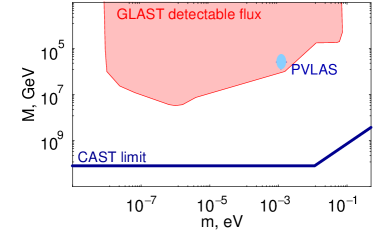
Figure 2: Axion parameter space. For the shaded region, GeV photon flux through the Sun detectable with GLAST at the solar occultations of 3C 279 is expected. The ellipse corresponds to PVLAS-motivated parameters pvlas . The values of $M$ above the thick line are disfavored by CAST CAST .

Inside the Sun, away from the resonance, the conversion probability is very small. Despite this, the high density and almost immediate absorption of any occasionally created photon may result in cumulative decrease of the axion flux. In the same adiabatic approximation, for the gamma-ray energies $E\lesssim 10$ GeV and for the paths not going very deep into the Sun (impact parameters $d\gtrsim 0.7R_{\odot}$), this cumulative effect does not reduce the number of axions in the beam by more than 10%. This means that for the parameters specified, a non-negligible part of the initial photon-axion mixture would travel through the optically thick regions in the form of axions and would convert back to photons at the solar surface. It is therefore possible that a gamma ray source would be able to shine through the Sun, although in practice only a fraction of photons would emerge.

To be more precise and to go beyond the adiabatic approximation, we integrate numerically the equations of motion along a path of several thousand kilometres through the Sun. Instead of explicitly solving the Schrödinger equation, it is better to go to the interaction representation and separate out the mixing that we are interested in from the normal propagating oscillation. This can be done by defining a density matrix $\rho=\Psi^{*}\Psi$ with an evolution equation raffelt ; deffayet

$$i\partial_{z}\rho=[\mathcal{M},\rho]-i{\cal D}\rho$$ (5)

where here we have simultaneously introduced a damping matrix $\cal{D}$ designed to take into account interactions between the photon part of the wavefuction and the particles inside the Sun. This damping matrix takes the form

$${\cal D}\equiv\left(\begin{array}[]{ccccccccc}\Gamma&\Gamma&\frac{1}{2}\Gamma\\ \Gamma&\Gamma&\frac{1}{2}\Gamma\\ \frac{1}{2}\Gamma&\frac{1}{2}\Gamma&0\end{array}\right)$$ (6)

where the inverse decay length $\Gamma=n_{e}\sigma$ and we again use the Bethe-Heitler cross section for the $\sigma$. We assume that the beam entering the Sun has a ratio of 2:1 photon:axion for the following reason. Figure 3 is a Hillas plot of the magnetic field of some typical gamma-ray sources vs. their size (the transient nature of gamma ray bursts means that one could not predict when to point the detector at the Sun so we have not included them on this plot.) All of the sources are larger in size than the oscillation length at maximal mixing ($l_{\rm osc}\sim M/B$) corresponding to their magnetic fields and the coupling of the PVLAS photon. A more detailed analysis would look at the coherence length of the magnetic field rather than the total extent of the object, but for the smaller objects with higher magnetic fields, one would expect these two length scales to be closer together. The right hand axis of figure 3 shows the energy necessary for maximum mixing to be achieved. The source we will be looking at in this paper is a quasi-stellar object, in other words an active galaxy, so we expect there to be strong mixing and many oscillation lengths in the source, and the high energy photons created should therefore be equal mixtures of both photon polarisations and the axion.

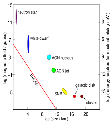
Figure 3: Hillas plot of the magnetic field of objects vs. their size. The oscillation length at maximal mixing for the PVLAS coupling $M=10^{5}$ GeV is plotted as a function of magnetic field (diagonal line). The right hand axis shows the photon energy required for maximal mixing as a function of magnetic field assuming the PVLAS coupling and mass $m=10^{-3}$ eV.

Figure 4 shows the actual mixing in action along a path through the Sun at a depth of 0.95 $R_{\odot}$.

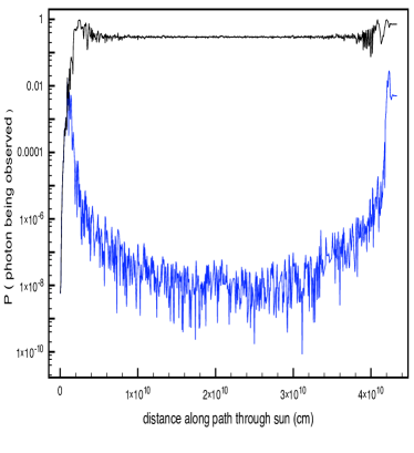
Figure 4: The probability of a photon emerging when a GeV PVLAS axion enters the Sun with an impact parameter 0.95 $R_{\odot}$. Upper curve: unrealistic case with photon cross section neglected. The two resonant regions can be clearly seen. Lower curve: the same but including photon interactions.

In figure 5 we plot the probability of a photon emerging as a function of the maximum depth along the path through the Sun for an axion mass of $10^{-3}$ eV and different values of the coupling $M$.

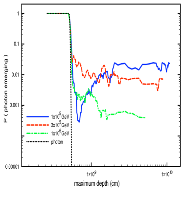
Figure 5: The probability of a GeV photon emerging for pseudoscalar mass $m=10^{-3}$ eV and different inverse coupling scales $M$. The dotted line bounds the maximal depths still transparent for GeV photons.

The results of the numerical solution are in rather good agreement with the analytical estimates presented above. In particular, the probability of gamma rays emerging from the Sun when a bright source passes behind it may be as high as 2% for GeV energy photons, if the interpretation of the PVLAS signal as an axion is valid, and even larger for the parameters shown in Fig. 2.

Let us turn now to observational constraints on gamma rays passing through the Sun. The only source in the EGRET catalogue 3EG occulted by the Sun is the quasi-stellar object 3C 279. EGRET observed the solar occultation of 3C 279 in 1991, in the viewing period 11.0. The QSO was in moderate state and was firmly detected in gamma rays during that viewing period 3EG .

The source was screened by the Sun for 8 hours 34 minutes on October 8, 1991 Planeph . The minimal impact parameter was $d=0.75R_{\odot}$.

We analysed the EGRET data following EGRET:like . The apparent flux of photons with energy $E\gtrsim$100  MeV from the location of 3C 279 during the occultation is $(6.2^{+3.7}_{-2.7})\cdot 10^{-7}$ cm^-2 s^-1, to be compared with the value obtained from the analysis of the rest of the same viewing period when the source is not behind the Sun which is $(8.6\pm 0.5)\cdot 10^{-7}$ cm^-2 s^-1. This latter result, obtained from our own analysis of the data, is in a very good agreement with the value quoted in the 3EG catalog 3EG for this period, $(7.94\pm 0.75)\cdot 10^{-7}$ cm^-2 s^-1. We see that a non-zero point-source flux from the location of 3C 279 during the occultation cannot be confirmed or excluded at the present level of statistics. Since such a non-zero flux could be the signal of a new elementary particle, this calls for future astronomical observations with more precise instruments. In particular GLAST is predicted to have a sensitivity of $3\times 10^{-8}$cm^-2s^-1 for the period of 8 hours glast . By looking at the same source when it is eclipsed by the sun, GLAST will therefore be able to rule out complete transparency to gamma rays. GLAST could also observe the partial transparency predicted in this paper, confirming the interpretation of the PVLAS data as a new particle.

Acknowledgments Discussions: L. Bergström, B. Irby, D. Gorbunov, V. Rubakov, G. Rubtsov, M. Tavani and P. Tinyakov. Funding: Vetenskapsrådet and PI (MF), Marie Curie program, RFBR grant 04-02-16386 and RAS Program “Solar activity” (TR), Russian Science Support Foundation, grants INTAS 03-51-5112 and NS-7293.2006.2, CERN (ST). Computers: Stockholm GLAST machines, INR cluster (RF gov.contract 02.445.11.7370), PI.

References

- (1) P. Sikivie, Phys. Rev. Lett. 51, 1415 (1983) [Erratum-ibid. 52, 695 (1984)]; Phys. Rev. D 32, 2988 (1985) [Erratum-ibid. D 36, 974 (1987)].
- (2) G. Raffelt and L. Stodolsky, Phys. Rev. D 37, 1237 (1988).
- (3) D. J. Thomson et al., J. Geophys. Res. 102 (1997) 14735.
- (4) E. Zavattini et al. [PVLAS Collaboration], Phys. Rev. Lett. 96 (2006) 110406
- (5) D. Kang et al. [CAST Collaboration], hep-ex/0605049.
- (6) E. Masso and J. Redondo, JCAP 0509 (2005) 015; Phys. Rev. Lett. 97 (2006) 151802.
- (7) M. Chaichian, M. M. Sheikh-Jabbari and A. Tureanu, hep-ph/0511323; P. Jain and S. Mandal, astro-ph/0512155; I. Antoniadis, A. Boyarsky and O. Ruchayskiy, hep-ph/0606306; T. Fukuyama and T. Kikuchi, hep-ph/0608228.
- (8) R. Rabadan, A. Ringwald and K. Sigurdson, Phys. Rev. Lett. 96 (2006) 110407
- (9) K. Zioutas et al., J. Phys. Conf. Ser. 39 (2006) 103 [arXiv:astro-ph/0603507].
- (10) A. Dupays et al., Phys. Rev. Lett. 95 (2005) 211302 [arXiv:astro-ph/0510324].
- (11) H. C. Spruit, Solar.Phys., 34, 277, (1974)
- (12) J. E. Vernazza, E. H. Avrett and R. Loeser, Astrophys. J. 45 635 (1981)
- (13) C. Deffayet, D. Harari, J. P. Uzan and M. Zaldarriaga, Phys. Rev. D 66, 043517 (2002)
- (14) R. C. Hartman et al., Astrophys. J. Supp. 123 (1999) 79.
- (15) J. Chapront, G. Francou, Ephemerides of planets between 1900 and 2100 (1998 update), ftp://cdsarc.u-strasbg.fr/pub/cats/VI/87
- (16) J. R. Mattox et al., Astrophys. J. 461 (1996) 396.
- (17) J. E. McEnery, I. V. Moskalenko and J. F. Ormes, astro-ph/0406250.