Computation of the Fourier parameters of RR Lyrae stars by template fitting

Abstract

Aims. Due to the importance of accurate Fourier parameters, we devise a method that is more appropriate for deriving these parameters on low-quality data than the traditional Fourier fitting.

Methods. Based on the accurate light curves of 248 fundamental mode RR Lyrae stars, we test the power of a full-fetched implementation of the template method in the computation of the Fourier decomposition. The applicability of the method is demonstrated also on datasets of filter passbands different from that of the template set.

Results. We examine in more detail the question of the estimation of Fourier-based iron abundance [Fe/H] and average brightness. We get, for example, for light curves sampled randomly in 30 data points with $\sigma=0.03$ mag observational noise that optimized direct Fourier fits yield $\sigma({\rm[Fe/H]})=0.33$, whereas the template fits result in $\sigma({\rm[Fe/H]})=0.18$. Tests made on the RR Lyrae database of the Large Magellanic Cloud (LMC) of the Optical Gravitational Lensing Experiment (OGLE) support the applicability of the method on real photometric time series. These tests also show that the dominant part of error in estimating the average brightness comes from other sources, most probably from crowding effects, even for under-sampled light curves.

1 Introduction

The method of Template Fitting (TF) is a widely used approach in data analysis. In astronomical applications we find examples from spectrum analysis (e.g., Bertone et al. 2004) to galaxy classification and redshift estimation (e.g., Wolf, Meisenheimer & Röser 2001; Padmanabhan et al. 2005). The method is based on the simple assumption that the population to be studied contains targets sharing the same topological properties as the members of the template set. The latter is defined as a set containing all possible ‘flavors’ of the given population and possessing accurately known parameter arrays – e.g., spectrum, redshift, etc. The actual implementation of the TF method ranges from the simple few-template direct match (e.g., Jones, Carney & Fulbright 1996; Layden 1998) to the more sophisticated Artificial Neural Network method (e.g., Collister & Lahav 2004).

Here we present a ‘brute force’ direct TF method that is aimed at the computation of the Fourier decompositions of fundamental mode RR Lyrae (RRab) stars. The goal of this investigation is to provide a reliable method for the computation of the Fourier decomposition of any observed RRab light curve even if observational noise or poor sampling impair standard Fourier decomposition. Our approach is different from that of Kanbur & Mariani (2004) and Tanvir et al. (2005), who employed principal component analysis (PCA) to parametrize the light curves of RR Lyrae and Cepheid variables. With the aid of PCA one is able to create a smaller set from the templates and represent the target by a low-degree (in some sense optimum) PCA decomposition. However, low-order PCA decompositions are often insufficient if more subtle features are required to fit (see also Fig. 2 of Tanvir et al. 2005). In addition, in the case of RR Lyrae stars, Blazhko effect further increases the possible types of light curves(see also Jurcsik, Benkő & Szeidl, 2002). Therefore, we are resorted to a method that is able to handle a large variety of light curves, flexible enough but does not ‘over-fit’ the data.

Compared to earlier related works on RR Lyrae stars, the present one utilizes a much larger template set, containing 248 accurate RRab light curves. The method is tested through a comparison with an optimized Fourier fit. We focus on the accuracy of the estimation of the iron abundance [Fe/H] based on the Fourier decomposition (Jurcsik & Kovács 1996, hereafter JK96, see also Kovács 2005) and on the determination of the period-luminosity-color (PLC) relation (Kovács & Walker 2001, hereafter KW01). Neither of these quantities can be accurately estimated with direct Fourier fit if the number of data points is low and the noise is high, such as in the case of the $V$ and $B$ band observations of OGLE (Soszynski et al. 2003). Furthermore, the success of any utilization of the color indices in the computation of the physical parameters (most importantly that of $T_{\rm eff}$) strongly depends on the accuracy by which we estimate average colors. As far as the computation of the Fourier-based [Fe/H] is concerned, here the accurate estimation of $\varphi_{31}$ is also important, because of the strong dependence of [Fe/H] on this quantity – see the application of the empirical [Fe/H] formula on the MACHO LMC data by Kunder et al. (2006). Current efforts in deriving [Fe/H] on large samples of stars in globular clusters and nearby galaxies from low/medium-dispersion spectroscopy (e.g., Sandstrom, Pilachowski & Saha 2001 [M3]; Gratton et al. 2004 [LMC]; Clementini et al. 2005a [NGC 6441]; Clementini et al. 2005b [Sculptor dwarf spheroidal galaxy]; Sollima et al. 2006 [$\omega$ Cen]) make the accurate computation of the Fourier decompositions of RRab stars even more interesting.

In the subsequent sections we describe the method, optimize the template function, discuss template completeness, investigate the effect of choosing different filter passbands for the target and template sets and test the accuracy of [Fe/H] and average magnitudes derived from the TF method. Finally, we present results based on a limited dataset from the OGLE RRab database.

2 The TF and the direct Fourier methods

In order to make a meaningful (and fair) comparison between the Fourier parameters derived from the TF method and those obtained from a straightforward Fourier fit, we need to perform the latter in an ‘optimum way’ (i.e., the way it would be done by a skilled data-analyst by checking the fit for different orders and avoiding – if possible – overshooting and appearance of strong wiggles for under-sampled light curves). First we describe our automated method for the Direct Fourier Fitting (DFF) and then give details on the Template Fourier Fitting (TFF).

In the case of DFF we tried to establish a set of criteria that results in ‘good looking’ fits and can be applied automatically, without further human inspection. Because we employ standard unweighted least squares Fourier fits, the only parameter by which we can influence the quality of the fit is the order of the Fourier sum. By scanning the orders from $1$ to $10$, we choose the highest order at which the following criteria are satisfied:

• The Fourier amplitudes are still ‘nearly’ monotonically decreasing (i.e. $A_{i-1}>f_{A}A_{i}$, where $f_{A}$ is one of our ‘trial and error’ parameters and is set equal to $1.2$, based on the inspection of the observed Fourier amplitudes of RRab stars – see Fig. 1).

• The unbiased estimate of the fitting accuracy (the r.m.s. of the residuals between the fit and the data) is minimum.

• The total amplitude of the fitted curve is not greater than $f_{T}A_{tot}$, where $A_{tot}$ is the total amplitude of the target signal and $f_{T}$ is our second empirical parameter, and is also chosen to be equal to $1.2$.

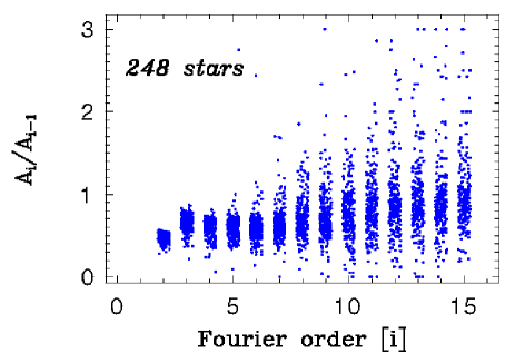
Figure 1: Amplitude ratios of the successive Fourier components of the 248 RRab stars of the basic dataset. For better visibility, data points related to the individual objects are shifted in the horizontal direction. Except for orders above 9–10, for most of the objects the amplitudes monotonically decrease with the increase of the order of the components.

These criteria make DFF reasonably stable for poorly sampled light curves, and produce accurate fit for well-sampled ones. We note that Ngeow et al. (2003) employed a somewhat similar method in deriving smooth and stable Fourier decompositions for Cepheid light curves. Their method employs ‘simulated annealing’ (see Press et al. 1992) constrained by the period dependence of the Fourier amplitudes of Cepheids (the so-called Hertzsprung progression).

For TFF, our approach is similar to that of Layden (1998), except that: (i) we use a much larger template set, based on individual variables and not on a limited set of visually selected classes; (ii) we allow low-degree polynomial transformation of the template in finding the best fit.

First we choose a set of Fourier decompositions derived from well-observed, densely sampled light curves. Such a set is available from our earlier studies on the $V$ band light curves of RRab stars (see the CDS archive of KW01). There are altogether 492 variables, with 105 stars from the Galactic field and the rest from various globular clusters and from the Sculptor dwarf galaxy. Because some of variables are poorly sampled, we apply the following selection criterion in order to employ only the best quality light curves. First we define the Quality Factor (QF) of a given light curve as a quantity proportional to the ratio of the amplitude $A_{1}$ of the first Fourier component to its simple error estimate, i.e.

$${\rm QF} = \sqrt{N}A_{1}/\sigma_{\rm fit}\hskip 5.69054pt,$$ (1)

where $N$ is the number of data points and $\sigma_{\rm fit}$ is the unbiased estimate of the standard deviation of the residuals of the fit. The quality control is established by requiring $\rm{QF}>{\rm QF_{\rm min}}$, where ${\rm{QF}_{\rm min}}$ is a preset threshold. By changing ${\rm QF_{\rm min}}$ from $100$ to $200$, the number of the remaining stars decreases from 336 to 193. Finally we decided to apply ${\rm QF_{\rm min}}=150$ and obtained a set of $251$ stars. The overwhelming majority of these stars have $N>100$, and there are only three stars with $N<40$. Since at lower number of data points there is a greater risk of having erroneous Fourier decompositions, we omit these three stars (FH Vul, IV Hya and NGC1841 V4). Finally we arrive to our basic dataset containing $248$ variables. We use this set as the template set throughout this paper.

Once the template set is selected, for a target light curve we find the best fitting template in the following way.

• Compute densely sampled folded light curves from the template Fourier decompositions. We denote these functions by {$x_{i,j}(\varphi)$}, where subscript $i$ stands for the array index in the folded light curve and $j$ refers to the template identification. Phase $\varphi$ of the template is arbitrary at this step.

• Compute folded light curve {$Y_{i}$} for the target.

• For each initial phase $\varphi$ and for each template, minimize the following quantity:

  $${\cal D}_{j}(\varphi) = {1\over N}\sum_{i=1}^{N}[Y_{i}-X_{i}(\varphi)]^{2}\hskip 5.69054pt,$$ (2)

  where

  $$X_{i}(\varphi)=\left\{\begin{array}[]{ll}c_{0}+x_{i,j}(\varphi)&\hskip 22.76219pt\mbox{if \ $M=0$}\\ \sum_{k=0}^{M}c_{k}x_{i,j}^{k}(\varphi)&\hskip 22.76219pt\mbox{if \ $M\gid 1$}\end{array}\right.$$

  Here $M$ denotes a preset polynomial degree, to be determined in Sect. 3 as a data quality-dependent parameter. While scanning $\varphi$, we employ quadratic interpolation for the template in order to get a good approximation for its value at the moments where the target is given.

• TFF is computed by the Fourier decomposition of that {$X_{i}(\varphi)$}, which minimizes ${\cal D}_{j}(\varphi)$ of Eq. (2).

• The above steps are to be supplemented by the ones to be discussed in Sect. 3 for the optimum choice of $M$.

Typically we use template light curves sampled in $300$ points and require an accuracy of $10^{-5}$ in the phase match between the target and template. The search for optimum phase is made iteratively, starting with some 50 phase steps. Execution time is not an issue with current several GHz machines.

One can construct other types of TF methods, by using different functional dependence of the target on the template members (e.g., linear or polynomial multi-template functions). However, in our approach we consider the current template set only as a subset of an ever growing master set that will be accumulated in the future. For this ideal set we might need only a scaling factor for a very precise fit of any target, because the master set will contain all ‘flavors’ of RRab stars and the fitting routine needs to perform the search only among the single template members. In addition, more complicated functional dependence would make the fitting procedure slower.

3 Template polynomial degree and completeness

Before testing the TFF method described in Sect. 2, it is necessary to determine the best polynomial degree $M$ to be used in the template transformation. Furthermore, it is also important to examine if the template set with the adopted TFF method is capable of reproducing all (or most of) the light curve ‘flavors’ observed among RRab stars. This latter property is connected to what we call ‘completeness’ and to be defined somewhat more precisely later in this section.

The purpose of introducing the polynomial template transformation is to increase our freedom in reaching higher accuracy in fitting targets. Obviously, employing a too high-degree polynomial may lead to instability, similarly as if we used high-order Fourier fit. Because the prime goal of the application of the template method is just to avoid this type of instability, we accept the lowest polynomial degree that yields fits of similar quality as the higher degree ones.

In order to rank the results obtained with various polynomial degrees, we need to define a function that characterizes the quality of the fit for an ensemble of targets. Using some average of the standard deviations of the fits to the individual targets is not satisfactory, because then, poorly fitted small-amplitude variables may stay hidden due to the small standard deviations associated with their small amplitudes. A possible normalization by the amplitude (see Eq. (1) for QF) may partially cure this problem, but we found more satisfactory to use a function that is independent of the amplitude and more closely related to our prime interest in deriving accurate phases. We introduce the following quantity to characterize the goodness of the fit

$${\rm RMS}(\Delta\varphi) = \biggl{[}{1\over 3}\sum_{k=2}^{4}(\Delta\varphi_{k1})^{2}\biggr{]}^{1\over 2}\hskip 5.69054pt,$$ (3)

where $\Delta\varphi_{k1}$ is the difference between the target and the best template-fitted phases. The epoch-independent phase is defined in the usual way $\varphi_{k1}=\varphi_{k}-k\varphi_{1}$ (Simon & Lee 1981). Notice that the above expression utilizes all three low-order phases, not only $\varphi_{31}$ that enters in the empirical formula for [Fe/H]. We think that using more phases makes the results more stable against statistical fluctuations. At the same time, adding high-order phases would make the above statistic biased toward small fitting errors, that we would like to avoid.

By using ${\rm RMS}(\Delta\varphi)$, the optimum polynomial degree $M$ is determined in the following way. For any fixed $M$ we start with the $248$ stars of the basic dataset and for each variable of this set we find the best fitting template selected from the remaining $247$ stars. The time series of the target is computed from the Fourier series given in the basic dataset for the target chosen. The time base of the sampling is taken arbitrarily as $12.3456P$, where $P$ is the period of the target. The sampling rate is quasi-uniform with a small randomness of the size of the exact uniform sampling. Tests are run both with and without noise added to the synthetic data. We note that other choices of the time base would also serve the purpose, except for near integer multiple of the period, when the chance of regular sampling of the phased light curve would be greater.

Once the best template (i.e., {$X_{i}(\varphi)$}, in Eq. (2)) is found, the resulting Fourier decomposition is compared with that of the target via Eq. (3). In this way at each fixed $M$ we get $248$ ${\rm RMS}(\Delta\varphi)$ values that can be analyzed statistically and compare with those obtained at other $M$ values.

The most straightforward way to compare the ${\rm RMS}(\Delta\varphi)$ values is to compute their probability distribution function (PDF). In Fig. 2 we show such functions computed for the noiseless (i.e., $\sigma=0.0$) simulations with $N=20$. As expected, the distribution functions become more narrow and concentrated at lower ${\rm RMS}(\Delta\varphi)$ values when $M$ is chosen to be low. From this test the optimum $M$ at $N=20$ is expected between $2$ and $4$ for noiseless data.

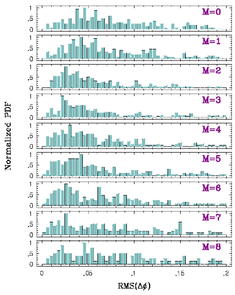
Figure 2: Probability distribution functions of the average phase differences ${\rm RMS}(\Delta\varphi)$ (Eq. 3) for test targets at various template polynomial degrees $M$. All target light curves were generated with $N=20$ data points. No noise is added. The test was performed on the basic dataset. Each PDF is normalized to its maximum. We draw attention to the narrowing of the PDFs at low $M$ values of $2$–$4$.

If we perform the above test at other values of $N$, then we get different values for the optimum $M$. This is understandable, because at low $N$ the high polynomial degree leads to stronger instabilities, whereas at high $N$ we are able to fit templates of high degree, thereby reaching higher accuracy. In order to get an estimate on the size of this shift of $M$, we performed additional tests with $N=15$, $N=40$ and $N=100$. For an easier comparison, instead of plotting PDFs, we compute the number of stars that have ${\rm RMS}(\Delta\varphi)$ greater than ${\rm RMS}_{\rm max}$, where the latter quantity is chosen in a way which ensures that, at least for some distribution functions, the number of stars satisfying this condition is small. From the inspection of Fig. 2 we choose ${\rm RMS}_{\rm max}=0.12$, because for weakly-spread distribution functions the tail seems to be separated from the bulk of the distribution at this value. (We note that our conclusion does not change by choosing other cutoff values in the range of $0.07$–$0.17$.)

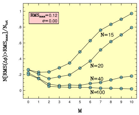
Figure 3: Dependence of the relative number of poorly fitted targets on the polynomial template degree $M$ and on the number of data points $N$ of the target time series. Tests were made on the basic dataset with $N_{\rm tot}=248$ stars. No noise was added to the synthetic data.

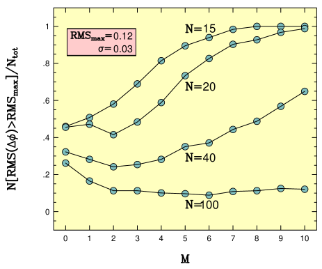
Figure 4: As in Fig. 3, but with added noise as given in the shaded box.

Fig. 3 shows that the size of the shift in the location of the minima of the functions is small for low $N$ values and we can still stay in $M=2$–$4$, with hitting the low and high boundaries at low and high $N$ values, respectively. For modest (or high) $N$ values the minima become shallower, therefore, there will not be much difference between choosing moderately low $M$ and the optimum one. However, it is clear that at large $N$ the minimum will be lower and gradually shifted to rather high $M$ values. On the other hand, these high-$N$, well-sampled cases are not interesting from the present point of view, because these are well-treated by standard Fourier fitting methods. (Exceptions are of course cases when high noise prohibits the traditional approach, and we will become better off again by using the template method at low $M$.)

To check the effect of noise on the optimum polynomial degree, we repeated the above test by adding moderate Gaussian noise of $\sigma=0.03$ mag to the synthetic target signals. The result is shown in Fig. 4. As expected, the properties observed at low $N$ in the noiseless case of Fig. 3 are shifted to higher $N$. At the same time, the low-$N$ signals get basically out of control at high $M$.

Due to the dependence of the optimum template polynomial degree on data quality, we need to examine this relation more closely. The data quality is characterized by the Signal-to-Noise Ratio (SNR), defined similarly to QF

$${\rm SNR} = \sqrt{N}A/\sigma_{\rm fit}\hskip 5.69054pt,$$ (4)

where $A$ is the total amplitude of the light variation, $\sigma_{\rm fit}$ is the unbiased estimate of the standard deviation of the residuals between the target and the fit. We performed tests similar to the ones described above and examined the behavior of ${\rm RMS}(\Delta\varphi)$ as a function of SNR and $M$. The SNR values were obtained from the results at $M=1$. For $N$, $M$ and $\sigma$ we took the following values: $N=15,\ 30,\ 45,\ 60,\ 90$, $M=0,\ 1,\ 2,\ 3,\ 4$ and $\sigma=0.0,\ 0.03,\ 0.06,\ 0.09$. Simulations corresponding to the same $M$ were averaged and plotted as functions of SNR in Fig. 5. The errors of the averages are about the size of the circles, except toward the low SNR end, where they increase to $0.1$–$0.2$. It is clear from this figure that the optimum polynomial degree is a function of SNR. Therefore, the TFF algorithm described in Sect. 2 is supplemented by the following steps in selecting the optimum polynomial degree.

• Compute SNR by applying TFF at $M=1$

• Choose the best $M$ depending on the computed SNR

  $$M=\left\{\begin{array}[]{ll}0,&\hskip 14.22636pt\mbox{if \ ${\rm SNR}<50.0$}\\ 1,&\hskip 14.22636pt\mbox{if \ $50.0\lid{\rm SNR}\lid 150.0$}\\ 2,&\hskip 14.22636pt\mbox{if \ ${\rm SNR}>150.0$}\end{array}\right.$$

• Compute TFF with $M$ determined above

We note that SNR can also be estimated by the simplest $M=0$ fit, but we choose $M=1$, because it yields a somewhat more consistent result (i.e., cleaner separation of the averages corresponding to the various $M$ values) and because of the unavoidable scaling in fitting light curves of different passbands (see Sect. 5). In the rest of this paper we use TFF with the above optimized $M$.

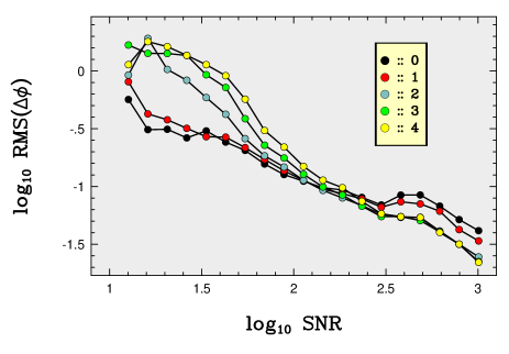
Figure 5: Dependence of the average of ${\rm RMS}(\Delta\varphi)$ on SNR at various template polynomial degree $M$ shown in the inset. The figure is based on simulated data described in the text in detail.

Next we address the question of template completeness. As already mentioned, we would like to measure the ability of the basic dataset in reproducing each member of the set with the aid of the TFF method. It is clear that we need to define the meaning of the word ‘reproduce’. Here, employing the same argument as earlier, we use ${\rm RMS}(\Delta\varphi)$ as a quantity characterizing the goodness of the fit. Then we say that the template set is complete at the level of ${\rm C}_{\rm TFF}$ at ${\rm RMS}_{\rm max}$, if the fraction of variables that satisfy the condition ${\rm RMS}(\Delta\varphi)<{\rm RMS}_{\rm max}$ is equal to ${\rm C}_{\rm TFF}$. Because the introduction of ${\rm C}_{\rm TFF}$ is aimed at to characterize the ability of the template set to ‘reproduce’ itself by using TFF, we generate noiseless, well-sampled, high-$N$ light curves to derive the dataset necessary for the computation of ${\rm C}_{\rm TFF}$. The result of is shown in Fig. 6. We see that the completeness is close to 90% at ${\rm RMS}_{\rm max}=0.1$ and reaches 95% at ${\rm RMS}_{\rm max}=0.15$. For some 80% of the stars we get matches with smaller RMS than $0.05$.

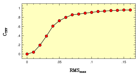
Figure 6: Completeness function of the TFF method. The symbol ${\rm C}_{\rm TFF}$ denotes the relative number of variables that have ${\rm RMS}(\Delta\varphi)<{\rm RMS}_{\rm max}$. We used the 248 light curves of the basic dataset with $N=200$ synthetic data points per object and polynomial degree $M=2$.

Although the above numbers indicate a reasonable completeness, we note that there are stars that stubbornly resist to accurate template fitting and prevent high completeness even at low-accuracy (e.g. for ${\rm RMS}_{\rm max}>0.15$). For example, variable M107~V12, cannot be fitted, yielding ${\rm RMS}(\Delta\varphi)=0.263$ and $\Delta\varphi_{31}=\varphi_{31}({\rm target})-\varphi_{31}({\rm template})=0.389$. There are some $15$ stars that have $|\Delta\varphi_{31}|>0.1$. The fact that some stars cannot be fitted even if their light curves are very densely sampled, can be explained by one (or some) of the following reasons: (i) the size of the current template set is small, and therefore, it is unable to reproduce some of the existing light curves with a desirable accuracy; (ii) some of the stars may exhibit long-periodic amplitude- and phase-modulations that result in discrepant template matches; (iii) the data on the targets were insufficient (too few data points, gaps in the folded light curves, etc.), that has led to inaccurate Fourier decompositions (in spite of these stars passing through our criteria for template membership); (iv) instrumental effects (e.g. daily or seasonal drifts) make the given light curve unique and therefore, not treatable by the template method; (v) some stars have periods close to integer ratios of one day, that again, may lead to unique light curves, especially if it is combined with property (iv). We think that from the present dataset we cannot decide which of the above effects is responsible for the outlier status of some of the stars (a closer examination of some of the outliers has shown that one can find examples/suspects for all these five possibilities). Considering that the current template set contains several stars with limited coverage either in time or in amount of data points, the existence of the few outliers is not surprising. It is clear that the present template set should be further extended by utilizing new observations and by leaving out objects with poor quality light curves.

To illustrate the difference between the matches produced by DFF and TFF at low number of data points, in Fig. 7 we show two examples. Although for other data distributions DFF might behave less erratically, the behavior shown is quite common at low number of data points. We note that in many cases the best matching template may have widely different period from that of the target. For instance, in the example shown, DX Del has a period of $0.47262$ d, whereas the best match is produced by $ω$~Cen V176, that has a period of $0.74275$ d. For RR Leo the situation is different, here we have $P=0.45239$ d for the target and $P=0.45930$ d for the matching template SW Aqr.

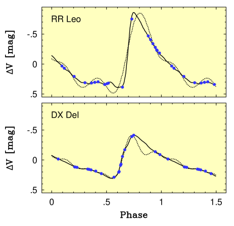
Figure 7: Examples of the performance of TFF at low data point numbers. Dots, dashed and continuous lines are for the noiseless synthetic data, DFF and TFF fits, respectively. The noiseless synthetic data have been obtained by the sparse sampling of the accurate observed light curve.

4 Estimation of the photometric [Fe/H]

From the point of view of applications, it is important to examine the accuracy of the TFF method in determining the photometric [Fe/H] with the aid of the formula of JK96. We used the basic dataset in generating simulated light curves with the following parameter values: $N=15,\ 30,\ 45,\ 60,\ 90$; $\sigma=0.0,\ 0.03,\ 0.06$. The polynomial degree $M$ was optimized as described in Sect. 3. For each $N$, $\sigma$ and for each star, we compute $\Delta{\rm[Fe/H]}$, the difference between the [Fe/H] values computed from the target and from the fitted light curves. From these values we derive: $\sigma(\Delta{\rm[Fe/H])}$, the standard deviation of the [Fe/H] differences; $R01$, the ratio of the stars with $|\Delta{\rm[Fe/H]|<0.1}$ to the total number of stars (i.e. to $248$); $T/D$, the ratio of the number of stars for which $|\Delta{\rm[Fe/H]|}$ is smaller for TFF than for DFF to the ones for which the opposite is true.

Table 1: Accuracy of the determination of [Fe/H].

$\sigma$	$N$	$\sigma_{\rm D}$	$\sigma_{\rm T}$	$R01_{\rm D}$	$R01_{\rm T}$	$T/D$
0.00	15	0.66	0.15	0.2	0.7	4.4
0.00	30	0.21	0.11	0.7	0.9	1.5
0.00	45	0.12	0.09	0.9	0.9	0.6
0.00	60	0.03	0.09	1.0	0.9	0.3
0.00	90	0.02	0.08	1.0	0.9	0.2
0.03	15	0.76	0.27	0.2	0.4	3.9
0.03	30	0.33	0.18	0.4	0.5	1.9
0.03	45	0.24	0.17	0.5	0.6	1.4
0.03	60	0.13	0.15	0.7	0.7	1.0
0.03	90	0.12	0.13	0.7	0.7	0.8
0.06	15	0.86	0.37	0.1	0.3	4.9
0.06	30	0.45	0.29	0.3	0.3	1.6
0.06	45	0.36	0.22	0.3	0.4	1.9
0.06	60	0.24	0.19	0.4	0.5	1.8
0.06	90	0.23	0.18	0.4	0.5	1.5

Note: $\sigma$: standard deviation of the noise added to the synthetic light curves that were generated from the template Fourier decompositions; $N$: number of data points; $\sigma_{\rm D}$: standard deviation of $\Delta{\rm[Fe/H]}_{\rm D}\equiv{\rm[Fe/H]}_{\rm target}-{\rm[Fe/H]}_{\rm DFF}$; $\sigma_{\rm T}$: as $\sigma_{\rm D}$, but for TFF; $R01_{\rm D}$: number of stars with $|\Delta{\rm[Fe/H]}_{\rm D}|<0.1$ divided by the total number of stars of $248$; $R01_{\rm T}$: as $R01_{\rm D}$ but for TFF; $T/D$: number of stars with $|\Delta{\rm[Fe/H]}_{\rm T}|<|\Delta{\rm[Fe/H]}_{\rm D}|$ divided by the number of stars satisfying the opposite inequality. The result is based on the $248$ stars of the basic dataset.

In Table 1 we show the average values obtained for these quantities for the two methods. The following conclusions can be drawn from this table:

• Except at low noise level and high (i.e. $\ga 45$) data point number, TFF always yields more accurate [Fe/H] values in the average sense.

• Within the above limit, the number of accurate [Fe/H] estimates (i.e. those with $|\Delta{\rm[Fe/H]|<0.1}$) is always larger for TFF.

• Within the above limit, the number of cases when TFF yields smaller error than DFF is always larger than that of the opposite situation.

• This better performance is especially well visible at higher noise levels.

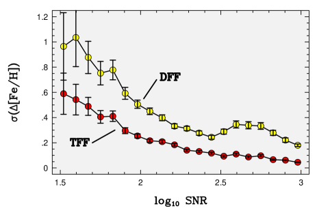
Figure 8: Standard deviation of the difference between the target and computed Fourier [Fe/H] values as a function of SNR. The test was made on the $248$ stars of the basic dataset. Error bars show the $\pm 1\sigma$ ranges of the means.

To make a comparison yet in another parameter domain, in Fig. 8 we plot the standard deviation of $\Delta{\rm[Fe/H]}$ as a function of SNR. Because the various simulations yield different individual SNR values, the total range of SNR was divided into $20$ bins and the standard deviations of the various $\Delta{\rm[Fe/H]}$ values within these bins have been computed. Except for low SNR values (i.e. for $\log{\rm SNR}<1.75$), all bins contain some 100–300 simulations (at $\log{\rm SNR}=1.5$ we have only 10). Although the scatter within the bins is very large, the averages are fairly accurately estimated and the difference between the two methods is clearly visible. This figure may give some guidance to a rough error estimation of the methods. In general, we may expect rather large errors – in the average sense – if $\log{\rm SNR}<2.0$. The average errors can be substantially decreased for DFF for $\log{\rm SNR}>2.0$ if we employ $3\sigma$ clipping on the derived [Fe/H] values. In this way the two methods will perform nearly in the same way for $\log{\rm SNR}>2.0$. The effect of $3\sigma$ clipping on TFF is minimal, because the number of outliers is much lower when TFF is employed. As an example, at $\log{\rm SNR}=2.75$, with $3\sigma$ clipping we loose $23$% of the stars in the case of the DFF method. The same figure for TFF is only $2$%.

5 Estimation of the average magnitudes in various colors

We test the applicability of the TFF method in estimating the average magnitudes of light curves observed in various wavebands. Unfortunately, the amount of good-quality multicolor data available for us is much lower than that of the single-color data. For simplicity, we take a set from the globular cluster data used by KW01 for the derivation of the PLC relation for RRab stars. The present set contains B, V and I light curves from globular clusters NGC 1851, 4499, 6362 and 6981. There are 95, 95 and 83 variables in B, V and in I colors, respectively. Although the amount and the quality of these data are less favorable than the ones used for testing the accuracy of the photometric [Fe/H], they are sufficient to get rough error estimates on the determination of average magnitudes by using different methods.

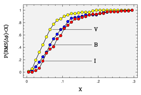
Figure 9: Empirical probability distribution functions of ${\rm RMS}(\Delta\varphi)$ for noiseless test signals drawn from samples of RRab stars of different wavebands. All test signals have $N=90$ data points. The TFF method with the basic dataset (available only in color V) is used in the computation of $\Delta\varphi$.

Table 2: Accuracy of the magnitude averages.

Band	AV/N	$15$	$30$	$45$	$60$	$90$
			$\sigma=0.0$
B:	AVE:	0.082	0.051	0.032	0.027	0.017
	DFF:	0.037	0.009	0.004	0.002	0.001
	TFF:	0.030	0.007	0.005	0.003	0.002
V:	AVE:	0.063	0.040	0.025	0.021	0.013
	DFF:	0.032	0.007	0.004	0.002	0.001
	TFF:	0.010	0.005	0.003	0.002	0.002
I:	AVE:	0.039	0.023	0.013	0.013	0.008
	DFF:	0.023	0.004	0.003	0.002	0.001
	TFF:	0.012	0.004	0.002	0.001	0.001
			$\sigma=0.03$
B:	AVE:	0.082	0.051	0.032	0.027	0.018
	DFF:	0.043	0.011	0.007	0.005	0.004
	TFF:	0.027	0.008	0.007	0.005	0.004
V:	AVE:	0.064	0.040	0.024	0.022	0.014
	DFF:	0.030	0.014	0.006	0.005	0.003
	TFF:	0.022	0.007	0.006	0.004	0.003
I:	AVE:	0.040	0.024	0.013	0.014	0.008
	DFF:	0.024	0.008	0.006	0.005	0.004
	TFF:	0.015	0.007	0.005	0.004	0.003
			$\sigma=0.06$
B:	AVE:	0.083	0.052	0.032	0.028	0.019
	DFF:	0.045	0.020	0.011	0.009	0.007
	TFF:	0.032	0.013	0.011	0.008	0.007
V:	AVE:	0.065	0.041	0.025	0.023	0.015
	DFF:	0.037	0.018	0.011	0.008	0.007
	TFF:	0.024	0.012	0.010	0.008	0.006
I:	AVE:	0.042	0.027	0.014	0.015	0.010
	DFF:	0.029	0.015	0.010	0.008	0.007
	TFF:	0.029	0.013	0.009	0.008	0.006

Note: Each item of data corresponds to the standard deviation of the $\Delta A_{0}$ values, as given by the difference between the average magnitude of the target and the one obtained by the application of the various methods (AVE denotes the simple arithmetic average). The tests are based on cluster RRab stars as given in the text. The result depends somewhat on the realization used, but this does not change the basic trends shown here.

Before discussing results on the average magnitudes, it is interesting to compare the accuracy of the fit in the different colors. As before, we use ${\rm RMS}(\Delta\varphi)$ to characterize the goodness of fit. Figure 9 shows the PDFs of this quantity for the different colors. As expected, the V-band data are fitted most accurately. The B and I data perform similarly, with a slight preference (but probably within the error limits of the present test) toward the B data. The fact that these, seemingly very similar light curves are not transformable by TFF, shows that they contain independent pieces of information on the pulsation. In the present context this result suggests to avoid the use of templates of different waveband from that of the target if we are aimed at the estimation of the Fourier decomposition with the aid of the TFF method.

In comparing the average magnitudes, we proceed in the same way as in the test of [Fe/H] in Sect. 4, except that now the target sets are limited on the cluster data mentioned above. The results are ranked on the basis of the standard deviations computed from the differences between the averages of the target (as given by the zero frequency constant in its accurate Fourier decomposition) and the estimated values. Table 2 shows the result of the computation for the three colors.

Although other realizations (determining the data distribution and noise) lead to somewhat different results, the following basic trends seen in the table survive.

• The simple arithmetic average (AVE) has the largest scatter and it is almost independent of the noise level.

• Within the statistical limits, TFF always performs better than DFF.

• If the number of data points is greater than $\sim 40$, TFF and DFF yield results of similar accuracy.

The near independence of AVE on the noise level is due to the fact that in the course of simple averaging the main source of error is the uneven distribution of data points in the phased light curve. It is seen that this effect is not negligible even at high number of data points. Therefore, for the accurate computation of the averages, simple averaging should never be used. Although Fourier decompositions are less accurately estimated for light curves of colors different from that of the template set, averages have nearly the same accuracy in all colors.

6 PLC estimates on artificial data

The correlation of the period and the reddening-free magnitude $W_{B-V}=V-R_{V}(B-V)$ is an important relation in estimating RR Lyrae distances from colors in the visual wavebands (Dickens & Saunders 1965; Kovács & Jurcsik 1997; KW01; see also Kovács 2003 for application in Baade-Wesselink analysis and Di Criscienzo, Marconi & Caputo 2004 for theoretical interpretation). Because of the large value of the selective absorption coefficient $R_{V}$, random errors in the estimated mean magnitudes become amplified in $W_{B-V}$ and thereby impair the accuracy by which we can employ the relation, among others, for distance determination. Therefore, it is worthwhile to test the effect of TFF in decreasing the error of $W_{B-V}$.

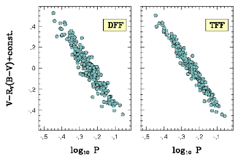
Figure 10: PLC relations computed from tests on the $248$ stars of the basic dataset. Test light curves were generated with $30$ data points and additive Gaussian noise of $0.03$ mag standard deviation. The selective absorption coefficient $R_{V}$ is set equal to $3.1$.

The test utilizes the $248$ stars of the basic dataset. For each star we generate test light curves in the following way:

• By using the Fourier decompositions of the $V$ light curves, compute magnitude-averaged $V$ and $B$ colors from Eqs. (5) and (6) of KW01.

• Compute zero-averaged synthetic light curves from the Fourier decompositions and add the averages determined above to obtain noiseless light curves, with averages that satisfy exactly the empirical PLC relation.

• Add Gaussian noise to the above noiseless light curves. The noise realizations used for the light curves with $V$ averages are different from the ones used for the light curves with the $B$ averages (however, they have the same standard deviation $\sigma$).

We note that the above generation of test light curves is not entirely consistent, because the noiseless $B$ light curves still have Fourier decompositions corresponding to the $V$ light curves. However, this inconsistency has only a small effect on the estimated average magnitudes as we have shown in Sect. 5 on a smaller set of real $B$ light curves.

In Fig. 10 we show an example of the improvement obtained by the application of TFF. The standard deviations around the best fitting straight lines are $0.064$ and $0.038$ for the DFF and TFF results, respectively. The derived slopes with their $1\sigma$ standard deviations of the means are the following: $-2.485\pm 0.022$ (DFF) and $-2.490\pm 0.013$ (TFF). These slopes are within the error limit of the empirical value of $-2.467$. Other realizations with higher noise also show the advantage of using TFF over DFF.

7 Tests on the OGLE LMC data

To test the applicability of TFF on real astronomical time series, we choose the RR Lyrae database of OGLE on LMC (Soszynski et al. 2003). Because the database contains more than 7000 entries and it is out of the scope of this paper to perform tests on all these stars, we choose a subset of it. This subset comprises fields # 4, 5 and 6 in the central, well-populated region of the LMC bar and fields # 17, 18, 19 and 20 in the far less-populated outermost part. Since the observational strategy of OGLE preferred the I (Cousins) band, the number of data points are different in the various wavebands. The overall number of data points, TFF fitting accuracy, QF and the total number of objects are (20, 0.07, 30, 1765), (40, 0.06, 35, 1886) and (500, 0.06, 78, 1947) in B, V and I colors, respectively. We note that the fitting accuracy and QF have substantial star-to-star scatter.

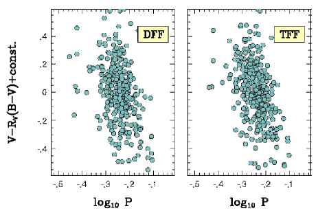
Figure 11: PLC relations computed from the DFF and TFF analyses of a subset of the OGLE database of RRab stars in the LMC. The selective absorption coefficient $R_{V}$ is set equal to $3.1$.

Two tests are performed. First we check how well the PLC relations of KW01 can be recovered, then we investigate the variation of the Fourier phase of the V light curves with the period. Because some light curves suffer from excessive noise (or some other types of deformation) we apply a parameter filter to keep only the good/reasonable quality light curves. In sorting out objects for the check of the PLC relation in (B,V) we require: ${\rm QF}>20.0$, $\sigma_{\rm fit}/\sqrt{N}<0.02$, $A_{1}>0.18$, $0.3<(B-V)_{0}<0.4$. Here, except for the color index, all criteria refer only to the V light curves. The dereddened color difference, $(B-V)_{0}$, is computed from the observed one with the assumption of $E_{\rm B-V}=0.1$ (see, e.g. Kovács 2000). There remained $318$ and $334$ stars passing these criteria in the DFF and TFF analyses, respectively.

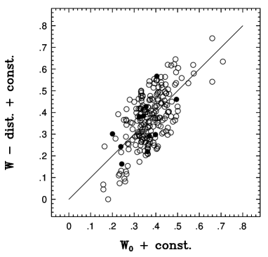
Figure 12: Correlation between $W_{0}=-1.59\log P$ and $W=V-3.1(B-V)$ (adjusted to field averages) for 218 RRab stars of selected LMC OGLE fields. The standard deviation of the fit is $0.096$ mag, the $1\sigma$ error of the slope is $0.08$. The $45\degr$ line is shown for reference. The result have been obtained by DFF with the top 100 most deviating stars clipped. Filled circles denote variables in field #20.

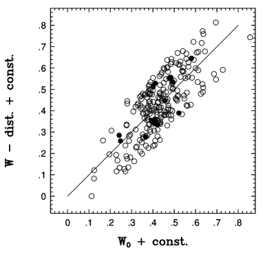
Figure 13: Correlation between $W_{0}=-2.33\log P$ and $W=V-3.1(B-V)$ (adjusted to field averages) for 234 RRab stars of selected LMC OGLE fields. The standard deviation of the fit is $0.092$ mag, the $1\sigma$ error of the slope is $0.05$. The $45\degr$ line is shown for reference. The result have been obtained by TFF with the top 100 most deviating stars clipped. Filled circles denote variables in field #20.

Figure 11 shows the resulting $\log P\rightarrow W_{\rm B-V}$ relations for these stars. We see that there is no particular improvement in the tightness of the relation whether using TFF or DFF. This is partially understandable, because, as Table 2 shows, we expect only moderate improvements in both colors. Although this improvement is too small to be easily visible in the above plot, we can test the difference by employing a direct search for the best single-parameter regression. To take into account the possible zero point differences between the different fields, we consider each field as a different ‘cluster’ and employ optimum (field-dependent) zero point shifts together with the uniform (i.e., field-independent) linear regression. We note that the zero point shifts were in general in the range of $\pm 0.05$ mag.

Figure 14: Low-order Fourier phases computed by DFF from the V light curves of 975 RRab stars of selected LMC OGLE fields. All stars have ${\rm QF}>20$ and $A_{1}<0.18$.

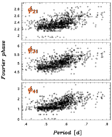
Figure 15: Low-order Fourier phases computed by TFF from the V light curves of 1056 RRab stars of selected LMC OGLE fields. All stars have ${\rm QF}>20$ and $A_{1}<0.18$.

Figures 12 and 13 show the resulting regressions. We used an iterative procedure in which at each step of the iteration we discarded the most deviating star from the best regression. We repeated this procedure 100 times. Of course, this excessive outlier selection is not justified statistically. However, our goal is to see which method is capable of estimating the functional dependence more accurately.

We found that in both cases the data quality was good enough for the code to select $P$ as the best regression parameter. This parameter was always the best among the other Fourier parameters at each stage of the iteration. However, as it is shown in the figure captions, TFF converged to a more accurate value of the slope of the $\log P\rightarrow W_{\rm B-V}$ relation. The slope obtained by DFF is completely out of range of the expected value of $-2.47$ (see KW01). It is also clear that the formal error substantially underestimates the true error in this case. The next best fitting Fourier parameter yielded standard deviations of $0.11$ and $0.13$ mag for the DFF and TFF methods, respectively. If we compare these values with the dispersions obtained for the regressions with $P$, we get that the increase is a factor of 1.16 for DFF, whereas it is 1.37 for TFF. This yields a higher significance for the correlation with $P$.

It is worthwhile to mention that Soszynski et al. (2003) did not derive the $\log P\rightarrow W_{\rm B-V}$ relation. However, they did it for the (V, I) colors, probably because of the higher accuracy of the data in these colors. We note that from the subset used in this paper we also derived consistent slopes for the $\log P\rightarrow W_{\rm V-I}$ relation. We got $-2.584\pm 0.032$ and $-2.662\pm 0.031$ from the DFF and TFF analyses, respectively. The two methods perform similarly also in other aspects, but the TFF sample contains some 40 more stars, due to the better quality of the TFF fits.

In both pairs of colors, the resulting regressions display larger dispersions than expected from standard statistical estimates. Although there might be several sources of the excessive scatter, crowding should definitely play a role (see Kiss & Bedding 2005). Our lower limit set for the $A_{1}$ amplitude is aimed at filtering out some of the blends in a crude way. Obviously, a more sophisticated method is needed to be more successful in filtering out blended variables.

A different test can be performed on the Fourier phases. This test is less stringent than the one presented above, because the quality of the result is judged from the tightness of the phase progression with the period, that is a good criterion only if there are reasonable pieces of evidence that the metallicity does not have a large scatter. This assumption is probably not a bad one for the LMC (e.g., Gratton et al. 2004 from spectroscopy of RRab stars; Kovács 2001, from double-mode stars). In Figs. 14 and 15 we show the progressions obtained for the V light curves of the selected fields mentioned at the beginning of this section. We see that the TFF data indeed exhibit a tighter correlation. Furthermore, the original number of stars of 1886 reduces in a less extent for TFF when various QF cutoff values are used. We also observe some horizontal structures in the TFF plots (see the sequences of circles at $\varphi_{21}=1.95$ and $2.15$). When lower QF cutoff is used, then these (and also some additional) structures become more visible. This indicates that the effect is partially due to poor data quality. However, visual inspection of the light curves producing these structures, and a similar test performed on the more substantial data in I color have shown that there are groups of stars producing nearly constant TFF phases even when large QF cutoff is used. Furthermore, because of the basic template set contains only 248 stars, it is possible that certain special structures observed by OGLE can be reproduced only by a few stars with very similar Fourier phases (which may yield constant phases if the template polynomial degree $M$ is equal to $0$ or $1$ – a common case for poor data quality).

8 Conclusion

We devised a full-fetched Template Fourier Fitting (TFF) method for the computation of the Fourier decompositions of undersampled, noisy fundamental mode RR Lyrae (RRab) light curves. The method can be extended to other types of variables, assuming that the corresponding template set is reasonably complete (i.e. it contains most of the ‘flavors’ of the potential targets). The main features of the method are as follows.

• Finds matches between the target and individual template members (i.e., it does not employ multi-template regressions);

• Fits templates to the target by applying polynomial transformation of the template;

• Optimizes the degree of the polynomial transformation between zero and two, depending on the data quality.

We performed a number of tests to investigate the range of applicability of the method. These tests included the estimation of: (i) the photometric iron abundance from the $\varphi_{31}$ Fourier phase and period $P$; (ii) the average magnitudes in various color bands; (iii) the period-luminosity-color relation. In all these tests TFF proved to perform better than an optimized Direct Fourier Fitting (DFF) method when the noise level was high or the number of data points was small. The two methods yield the same solution for light curves of high Signal-to-Noise Ratio (SNR). For example, when estimating [Fe/H] from light curves with $30$ data points we expect a factor of two increase in the accuracy of [Fe/H] if the standard deviation $\sigma$ of the noise is lower than $0.03$. For higher noise levels, TFF remains to be more accurate up to fairly high number of data points (e.g. with $\sigma=0.06$ we get better result with TFF even at $N\sim 100$).

When applied to a subset of the OGLE RR Lyrae database on the LMC (see Soszynski et al. 2003), TFF produces statistically more significant period-luminosity-color relation for (B, V) colors, although the significance of the relation still remains marginal on this subset. For (V, I) colors we get the same, statistically significant relation from both DFF and TFF. Nevertheless, the dispersion of the relations are high in all colors, suggesting the importance of crowding effects.

The stable performance of TFF for undersampled and noisy light curves makes it suitable to revisit problems such as the RR Lyrae metallicities in globular clusters and in galaxies (e.g. in the Magellanic Clouds) or the determination of average colors and empirical relations. With the various large-scale surveys (microlensing, variability, transit, etc.) there is an increase in the number of the good- and bad-quality light curves alike. Therefore, we expect TFF a useful supplementary method to the traditional Fourier fitting.

- (1) Bertone, E., Buzzoni, A., Chávez, M. & Rodríguez-Merino, L. H. 2004, AJ, 128, 829
- (2) Clementini, G., Gratton, R. G., Bragaglia, A., Ripepi, V., Fiorenzano, A. F. M., Held, E. V. & Carretta, E. 2005a, ApJ, 630, 145
- (3) Clementini, G., Ripepi, V., Bragaglia, A., Fiorenzano, A. F. M., Held, E. V. & Gratton, R. G. 2005b, MNRAS, 363, 734
- (4) Collister, A. A. & Lahav, O. 2004, PASP, 116, 345
- (5) Di Criscienzo, M., Marconi, M. & Caputo, F. 2004, ApJ, 612, 1092
- (6) Dickens, R. J. & Saunders, J. 1965, Roy. Obs. Bull., No. 101
- (7) Gratton, R. G.; Bragaglia, A., Clementini, G., Carretta, E., Di Fabrizio, L., Maio, M. & Taribello, E. 2004, A&A, 421, 937
- (8) Jones, R. V., Carney, B. W. & Fulbright, J. P. 1996, PASP, 108, 877
- (9) Jurcsik, J., Benkő, J. M. & Szeidl, B., 2002, A&A, 390, 133
- (10) Jurcsik, J. & Kovács, G. 1996, A&A, 312, 111 (JK96)
- (11) Kanbur, S. M. & Mariani, H. 2004, MNRAS, 355, 1361
- (12) Kiss, L. L. & Bedding, T. R. 2005, MNRAS, 358, 883
- (13) Kovács, G. & Jurcsik, J. 1997, A&A, 322, 218
- (14) Kovács, G. 2000, A&A, 363, L1
- (15) Kovács, G. 2001, A&A, 375, 469
- (16) Kovács, G. & Walker, A. R. 2001, A&A, 371, 579 (KW01)
- (17) Kovács, G. 2003, MNRAS, 342, L58
- (18) Kovács, G. 2005, A&A, 438, 227
- (19) Kunder, A. M., Chaboyer, B., Popowski, P., Nikolaev, S., Cook, K. H. 2006, PASPC, 349, 273
- (20) Layden, A. C. 1998, AJ, 115, 193
- (21) Ngeow, C-C., Kanbur, S. M., Nikolaev, S., Tanvir, N. R. & Hendry, M. A. 2003, ApJ, 586, 959
- (22) Padmanabhan, N., Budavári, T., Schlegel, D. J. et al. 2005, MNRAS, 359, 237
- (23) Press, W. H., Teukolsky, S. A., Vetterling, W. T., & Flannery, B. P., 1992, Numerical Recipes, 2nd edn., Cambridge Univ. Press, Cambridge, p. 292.
- (24) Sandstrom, K., Pilachowski, C. A. & Saha, A. 2001, AJ, 122, 3212
- (25) Simon, N. R. & Lee, A. S. 1981, ApJ, 248, 291
- (26) Sollima, A., Borissova, J., Catelan, M., Smith, H. A., Minniti, D., Cacciari, C., & Ferraro, F. R. 2006, ApJ, 640, L43
- (27) Soszynski, I., Udalski, A., Szymanski, M., Kubiak, M., Pietrzynski, G., Wozniak, P., Zebrun, K., Szewczyk, O. & Wyrzykowski, L. 2003, Acta Astron., 53, 93
- (28) Tanvir, N. R., Hendry, M. A., Watkins, A., Kanbur, S. M., Berdnikov, L. N. & Ngeow, C. C. 2005, MNRAS, 363, 749
- (29) Wolf, C., Meisenheimer, K. & Röser, H. J. 2001, A&A, 365, 660