Quintessence reconstructed: new constraints and tracker viability

Abstract

We update and extend our previous work reconstructing the potential of a quintessence field from current observational data. We extend the cosmological dataset to include new supernova data, plus information from the cosmic microwave background and from baryon acoustic oscillations. We extend the modelling by considering Padé approximant expansions as well as Taylor series, and by using observations to assess the viability of the tracker hypothesis. We find that parameter constraints have improved by a factor of two, with a strengthening of the preference of the cosmological constant over evolving quintessence models. Present data show some signs, though inconclusive, of favouring tracker models over non-tracker models under our assumptions.

I Introduction

The nature of dark energy in our Universe remains unknown, and is likely to be the subject of intense observational attention over the coming decade DETF . While a pure cosmological constant remains the simplest interpretation of present data, a leading alternative possibility is the quintessence paradigm, whereby the observed acceleration is driven by the potential energy of a single canonically-normalized scalar field quint (for extensive reviews of dark energy see Ref. reviews ). In this paper, we work under the assumption that quintessence is a valid description of observational data (an assumption to be tested separately), and seek to impose optimal constraints on the model via exact numerical computation. Our work provides an implementation of quintessence potential reconstruction, a subject developed by several authors rec ; dalyrec ; oldppr , and by assuming a particular physical model for dark energy is distinct from parameterized equation of state methods for reconstructing dark energy.

In a previous paper oldppr , we carried out a direct reconstruction of the quintessence potential based on the supernova type Ia (SNIa) luminosity–redshift measurements made/collated by Riess et al. riess . The present paper updates and extends that work in three ways:

1. We include additional data coming from cosmic microwave background (CMB) anisotropies wmap3 and baryon acoustic oscillations sdssbao , as well as using newer supernova data from the SuperNova Legacy Survey (SNLS) snls . We do not use constraints from the growth rate of structure, which are not yet competitive with the data we do use.

2. Where previously we approximated the quintessence potential via a Taylor series, we now additionally explore use of Padé approximant expansions in order to test robustness under choice of expansion.

3. By studying the dynamical properties of models permitted by the data, we assess whether current observations favour or disfavour the hypothesis that the quintessence field is of tracker form, hence potentially addressing the coincidence problem.

As we were completing this paper, a closely-related paper was submitted by Huterer and Peiris HP , who also reconstruct quintessence potentials from a similar compilation of current data. Although phrased in the language of flow equations, their approach, like ours here and in Ref. oldppr , amounts to fitting the coefficients of a Taylor expansion of the potential. They do not consider Padé approximants. Their approach implies different priors for the parameters than the ones used in this paper, and they treat the scalar field velocity a little differently. Our results appear in good agreement, in particular our determination that present data mildly favour tracker models over non-tracker models concurring with their conclusion that freezing models are mildly preferred to thawing ones (in the terminology of Ref. CL ).

II Formalism

II.1 Cosmological model

We quickly review the set-up of Ref. oldppr , which is conceptually straightforward. We assume that the quintessence field $\phi$ has a potential $V(\phi)$, which we expand in a series about the present value of the field that is taken (without loss of generality) to be zero. The quintessence field obeys the equation

$$\ddot{\phi}+3H\dot{\phi}=-\frac{dV}{d\phi}\,,$$ (1)

with the Hubble parameter $H$ given by the Friedmann equation

$$H^{2}=\frac{8\pi G}{3}\left(\rho_{{\rm m}}+\rho_{\rm\phi}\right)\,.$$ (2)

Here $\rho_{{\rm m}}$ is the matter density and $\rho_{\rm\phi}=\dot{\phi}^{2}/2+V(\phi)$ the quintessence density. We assume spatial flatness throughout (as motivated by CMB measurements and the inflationary paradigm), though the generalization to the non-flat case would be straightforward. Since then $\Omega_{\rm m}+\Omega_{\phi}=1$ we have the present boundary condition

$$\dot{\phi}_{\rm 0}=\pm\sqrt{2\left[(1-\Omega_{\rm m})\rho_{\rm c,0}-V(\phi_{0})\right]}\,,$$ (3)

where subscript ‘0’ indicates present value, and $\rho_{{\rm c}}$ is the critical density. An important quantity, which determines the cosmological effects we consider from the quintessence field, is the equation of state

$$w_{\phi}\equiv\frac{p_{\phi}}{\rho_{\phi}}=\frac{\dot{\phi}^{2}/2-V(\phi)}{\dot{\phi}^{2}/2+V(\phi)}\,.$$ (4)

The priors we assume for our cosmology are

$$\Omega_{\rm total} = 1\,,$$ (5)

$$\Omega_{\rm m} \geq 0\,,$$ (6)

$$\Omega_{\rm kin} \leq 1\,,$$ (7)

$$\Omega_{\rm kin}(z\geq 1) < 0.5\,.$$ (8)

where $\Omega_{\rm kin}=8\pi G\dot{\phi}^{2}/6H^{2}$ is the fraction of critical energy density in field kinetic energy density. The last condition is a means of encoding that the field should not interfere too much with structure formation (as we do not use data sensitive to that), and is discussed further in our previous paper oldppr . The constraint on $\Omega_{\rm kin}$ is in practice applied up to the highest redshift for which we have data points, i.e. using CMB information $z=1089$. When we use supernova data only, the upper limit is $z=2$, as in our previous study.

II.2 Parameterizations and priors

To explore the space of potentials, we need to assume some functional form for the potential. We choose two classes of expansions, a Taylor series, and a Padé series, to parameterize the potential function $V(\phi)$. In the absence of a theoretical bias for the functional form of the potential, these expansions seem suitably general and simple to provide a reasonably fair sampling of the space of potential functions.

II.2.1 Taylor series

As in our previous study, we use a Taylor series to model the potential $V(\phi)$ as

$$V(\phi)=V_{0}+V_{1}\phi+V_{2}\phi^{2}+\ldots$$ (9)

where $\phi$ is in units of the reduced Planck mass $M_{\rm P}$ with $\phi$ presently zero. We will refer to a constant potential with non-zero kinetic energy allowed as a skater model, after Linder in Ref. linderskater .

We put the following flat priors on the parameters:

$$V_{0}\geq 0\,,\quad|V_{1}|\leq 2\,,\quad|V_{2}|\leq 5\,.$$ (10)

These priors are irrelevant for parameter estimation, as they are significantly broader than the high-likelihood region (this also applies to the corresponding priors for Padé series below). However, to assess how favoured tracker behaviour is, we do need to put some limits, so that we can sample a finite region of the prior parameter space (see further in Section IV.3.2).

II.2.2 Padé series

In addition to the Taylor series expansion, in this paper we also use Padé approximant expansions in order to test the robustness of results to the method used. Padé approximants are rational functions of the form

$$R_{M/N}(\phi)=\frac{\sum_{i=0}^{M}a_{i}\phi^{i}}{1+\sum_{j=1}^{N}b_{j}\phi^{j}}\,,$$ (11)

that can be used to approximate functions. These approximants typically have better-behaved asymptotics, i.e. stay closer to the approximated function, than Taylor expansions because of their rational structure. An extensive exposé on Padé approximants can be found in Ref. pade . For our study, we will assume

$$V(\phi)=R_{M/N}(\phi)\,,$$ (12)

where again $\phi$ is in units of $M_{\rm P}$ with $\phi$ presently zero. Specifically, we use Padé series $R_{0/1}$, $R_{1/1}$ and $R_{0/2}$, as these form an exhaustive set of lowest order and next-to-lowest order non-trivial expansions with two or three parameters. Higher orders are unmotivated given the known difficulty for data to constrain more than two dark energy/quintessence evolution parameters linderhowmany ; oldppr ; Maor:2002rd (as will also be evident from our results).

Padé series have poles, but, as will be discussed in the Results Section, data constrains models so that the presence of poles is not felt.

To enable comparison between our results for the two different parameterization classes, the priors for the Padé series case are set by evaluating the MacLaurin expansion of the Padé series, identifying the order coefficients, and using the Taylor-series priors for those, i.e.

$$a_{0} = V_{0}\,,$$ (13)

$$a_{1}-a_{0}b_{1} = V_{1}\,,$$ (14)

$$b_{1}(a_{0}b_{1}-a_{1})-a_{0}b_{2} = V_{2}\,.$$ (15)

This does not limit us to a finite region, so we additionally require $|b_{1}|\leq 2$.

II.3 Tracker potentials

Cosmological tracker potentials/solutions have been studied in detail by numerous authors quint ; reftrack ; steintrack ; bludman ; linderpaths . These potentials are such that the late-time evolution of the field can be essentially independent of initial conditions, thus providing a possible solution to the coincidence problem. This behaviour is achieved through a type of dynamical attractor solution, and the conditions for it to be possible given a particular potential have been given and studied in detail by Steinhardt et al. steintrack . Defining $\Gamma\equiv V^{\prime\prime}V/V^{\prime 2}$, where prime denotes a derivative with respect to the field, the two sufficient conditions for a potential to possess a tracker solution are

$$\Gamma > 1-\frac{1-w_{\rm b}}{6+2w_{\rm b}}\,,$$ (16)

$$\left|\Gamma^{-1}\frac{d\Gamma}{d\ln a}\right| = \left|\frac{d\phi}{d\ln a}\left(\frac{V^{\prime}}{V}+\frac{V^{\prime\prime\prime}}{V^{\prime\prime}}-2\frac{V^{\prime\prime}}{V^{\prime}}\right)\right|\ll 1\,.\quad$$ (17)

The first of these conditions ensures convergence to the tracker solution (i.e. perturbations away from it are suppressed), and the second ensures an adiabatic evolution of the field that is necessary for the first condition to be applicable (and is what one would expect of a function that is to maintain a dynamical attractor independent of initial conditions).

If these conditions are fulfilled, the field will eventually approach the tracker solution (unless the initial quintessence energy density is too low), and the equation of state will then evolve according to

$$w_{\phi}\approx w_{\rm tracker}=\frac{w_{\rm b}-2(\Gamma-1)}{1+2(\Gamma-1)}\,,$$ (18)

possibly breaking away from the tracker solution if either of the conditions later become violated. In assessing whether tracking is taking place, one also has to check whether the actual evolution on the tracker potential corresponds closely to the tracker solution. An illustration of tracker behaviour can be seen in Fig. 1.

We additionally impose the condition $w_{\phi}<w_{\rm b}$, where $w_{\rm b}$ is the background energy density. This is to ensure a possible solution of the coincidence problem by having the dark energy density grow with respect to the matter. This third condition is usually avoided by specifying the tracker condition as $\Gamma>1$ rather than Eq. (16). The reason for not choosing $\Gamma>1$ as our condition is related to our numerical treatment, and is discussed further in Section IV.3.1.

As we need a non-zero second derivative of the potential with respect to the field for $\Gamma$ to fulfil the tracker conditions, we restrict ourselves to the quadratic potential and the Padé series for the tracker viability analysis.

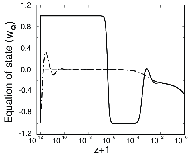
Figure 1: Examples of the behaviour of the equation of state (here called $w_{\rm Q}$) for a tracker potential. The oscillating curves correspond to higher (solid) and slightly lower (dash-dotted) initial conditions at high redshift for $\rho_{\phi}$ compared to the tracker solution value. The initial velocity at high redshift is assumed to be zero. The amplitude of oscillations in $w(z)$ around the tracker solution (thin-dashed curve originating at $w_{\rm Q}=0$) decays exponentially with decreasing $\ln(1+z)$, and the evolution thus approaches the tracker solution regardless of the different initial conditions. Although not directly corresponding to our models, the figure illustrates qualitatively the tracker property. Reproduced from Ref. steintrack .

III Observables

The observables used are essentially geometric and are hence related to the comoving distance for an FRW cosmology described by the parameter vector $\mathbf{\Theta}$, given by

$$r(z;\mathbf{\Theta})=H_{0}^{-1}\int_{0}^{z}\frac{{\rm d}z^{\prime}}{E(z^{\prime};\mathbf{\Theta})}\,$$ (19)

where

$$E(z;\mathbf{\Theta})=\left[\Omega_{\rm m}(1+z)^{3}+(1-\Omega_{\rm m})e^{F(z;\mathbf{\Theta})}\right]^{1/2}$$ (20)

and

$$F(z;\mathbf{\Theta})=3\int_{0}^{z}\left(1+w_{\phi}(z^{\prime};\mathbf{\Theta})\right){\rm d}\ln(1+z^{\prime})\,.$$ (21)

In accordance with our assumptions, these expressions assume zero curvature and that quintessence and non-relativistic matter are the only relevant components for the redshifts we consider.

We have not included growth-of-structure observations, which are not yet competitive with the measures we do use (see e.g. Ref. wangkratochvil for a directly-comparable example).

III.1 SNIa luminosity–redshift relation

The luminosity distance is given by

$$d_{\rm L}(z;\mathbf{\Theta})=\frac{\mathcal{D}_{\rm L}(z;\mathbf{\Theta})}{H_{0}}=(1+z)r(z;\mathbf{\Theta})\,.$$ (22)

The apparent magnitude $m(z;\mathbf{\Theta})$ of a type Ia supernova can be expressed as

$$m(z;\mathbf{\Theta})=M+5\log_{10}\frac{d_{\rm L}(z;\mathbf{\Theta})}{\rm Mpc}+25\,,$$ (23)

where $M$ is the absolute magnitude of SNIa (supposing they are standard candles). This can be rewritten as

$$m(z;\mathbf{\Theta})=\mathcal{M}+5\log_{10}\mathcal{D}_{\rm L}(z;\mathbf{\Theta})\,,$$ (24)

where $\mathcal{M}=M-5\log_{10}\left(H_{\rm 0}\,\,{\rm Mpc}\right)+25=M-5\log_{10}(h_{70})+43.16$ [where $h_{70}=H_{0}/(70\,{\rm km/s/Mpc})$]. Note that some authors define this quantity somewhat differently.

We use the 115 measurements of $m(z)$ measured/compiled by the SNLS team snls , covering the redshift range $z=0.015$ to $z=1.01$. The observed magnitudes (indexed by $i$) are given by

$$m_{i}=m^{*}_{{\rm B},i}+\alpha(s_{i}-1)-\beta c_{i}$$ (25)

where $m^{*}_{\rm B}$ is the rest-frame B-band magnitude at maximum B-band luminosity, and $s$ and $c$ are the shape and color parameters. These are derived from the light-curve fits and are reported by the SNLS team. The parameters $\alpha$ and $\beta$ are free parameters and should be varied in cosmological fits. However, as they are independent of cosmology fouchezpc , we fix them to the SNLS best-fit values

$$\alpha = 1.52\pm 0.14\,,$$ (26)

$$\beta = 1.57\pm 0.15\,,$$ (27)

without introducing any bias, and include their uncertainty in the magnitude uncertainties we use.

For comparison to our previous paper where the parameter $\eta$ is used, the parameter $\mathcal{M}=M^{*}_{\rm Riess}-\eta$, with $M^{*}_{\rm Riess}$ the estimate of intrinsic supernova magnitude in Riess et al. riess .

III.2 CMB peak-shift parameter

The CMB peak-shift parameter peakshift

$$\mathcal{R}(z_{\rm dec};\mathbf{\Theta})=\sqrt{\Omega_{\rm m}}H_{0}r(z_{\rm dec};\mathbf{\Theta})$$ (28)

measures an overall linear shift of the CMB power spectrum in multipole space, induced by the effect $\Omega_{\phi}$ has on the angular-diameter distance to the surface of last scattering at $z=z_{\rm dec}$. The position of the first power spectrum peak is essentially a measure of this distance.

We use the recent WMAP3 data wmap3 as analyzed by Wang and Mukherjee wangr , who found

$$\mathcal{R}(z_{\rm dec}=1089)=1.70\pm 0.03\,.$$ (29)

III.3 Baryon acoustic peak

The standard Big Bang scenario predicts that close to the surface of last scattering, baryons and photons act as a fluid with acoustic oscillations from the competition between gravitational attraction and radiation pressure. As the photons decouple, these acoustic oscillations should be frozen in the baryon and dark matter distributions. One would thus expect an excess of power in the power spectrum of luminous matter at a scale corresponding to the acoustic scale at last scattering (see e.g. Ref. baoth and references therein). Independent first detections of this baryon acoustic peak were made by the Sloan Digital Sky Survey (SDSS) sdssbao and the 2dF galaxy redshift survey 2dfbao . The SDSS team defined a distance quantity

$$A(z_{\rm BAO};\mathbf{\Theta})=\sqrt{\Omega_{\rm m}}\left(\frac{H_{0}^{2}r^{2}(z_{\rm BAO};\mathbf{\Theta})}{z^{2}_{\rm BAO}E(z_{\rm BAO};\mathbf{\Theta})}\right)^{1/3}\,,$$ (30)

which we will use for our analysis. The measurement (independent of dark energy model) from the SDSS luminous red galaxy power spectrum is sdssbao

$$A(z_{\rm BAO}=0.35)=0.469\left(\frac{n_{\rm S}}{0.98}\right)^{-0.35}\pm 0.017\,,$$ (31)

which, assuming the WMAP3 mean value $n_{\rm S}=0.95$ wmap3 , yields $A(z=0.35)=0.474\pm 0.017$.

IV Data analysis

IV.1 Parameter estimation

The parameter space we study will be

$$\mathbf{\Theta}=(\mathcal{M},\dot{\phi}_{\rm 0},\mbox{potential parameters})\,,$$ (32)

and we will consistently let $D$ denote the number of free parameters in a model. The parameter estimation is carried out using an MCMC approach, as outlined in our previous paper oldppr . The posterior probability of the parameters $\mathbf{\Theta}$, given the data and a prior probability distribution $\Pi(\mathbf{\Theta})$, is

$$P(\mathbf{\Theta}|{\rm data})=\frac{1}{{\cal Z}}e^{-\left(\chi_{\rm SNIa}^{2}(\mathbf{\Theta})+\chi_{\rm CMB}^{2}(\mathbf{\Theta})+\chi_{\rm BAO}^{2}(\mathbf{\Theta})\right)/2}\Pi(\mathbf{\Theta})\,,$$ (33)

where

$$\chi_{\rm SNIa}^{2}(\mathbf{\Theta}) = \sum_{i=1}^{N_{\rm SNIa}}\frac{\left(m_{i}-m(z_{i};\mathbf{\Theta})\right)^{2}}{\sigma_{i}^{2}}\,,$$ (34)

$$\chi_{\rm CMB}^{2}(\mathbf{\Theta}) = \frac{\left(\mathcal{R}_{\rm obs}-\mathcal{R}(z_{\rm dec};\mathbf{\Theta})\right)^{2}}{\sigma_{\mathcal{R}}^{2}}\,,$$ (35)

$$\chi_{\rm BAO}^{2}(\mathbf{\Theta}) = \frac{\left(A_{\rm obs}-A(z_{\rm BAO};\mathbf{\Theta})\right)^{2}}{\sigma_{\rm A}^{2}}\,.$$ (36)

Here, we sum over all $N_{\rm SNIa}$ data points for the SNIa data, and ${\cal Z}~{}=~{}\int{\cal L}({\rm data}|\mathbf{\Theta})\Pi(\mathbf{\Theta}){\rm d}\mathbf{\Theta}$ is a normalization constant, irrelevant for parameter fitting. Overall, we have 115(SNIa)+1(CMB)+1(BAO) data points.

IV.2 Model selection

Separate from the question of parameter estimation is the question of parameter necessity, i.e. model selection. We again employ an approximate model selection criterion, the Bayesian Information Criterion (BIC) Schwarz ; Lid , given by

$$\mathrm{BIC}=-2\ln{\cal L}_{{\rm max}}+D\ln N\,,$$ (37)

where ${\cal L}_{{\rm max}}$ is the likelihood of the best-fitting parameters for that model, $D$ the number of model parameters, and $N$ the number of datapoints used in the fit. Models are ranked with the lowest value of the BIC indicating the preferred model. A difference of two for the BIC is regarded as positive evidence, and of six or more as strong evidence, against the model with the larger value jeff ; Muk98 . The BIC has also been deployed for dark energy model selection in Ref. darkBIC .

IV.3 Tracker viability

IV.3.1 Identifying tracker solutions

To classify general scalar field evolutions as coming from a tracker potential capable of solving the coincidence problem or not, we need to test for both tracker conditions and whether the field evolves according to the tracker solution. As these conditions are approximate in nature, we must specify some $\epsilon\geq 0,\delta\geq 0$ such that if

$$\Gamma > 1-\frac{1-w_{\rm b}}{6+2w_{\rm b}}\,,$$ (38)

$$\left|\Gamma^{-1}\frac{d\Gamma}{d\ln a}\right| < \epsilon\,,$$ (39)

$$\left|w_{\phi}-w_{\rm tracker}\right| < \delta\,,$$ (40)

$$w_{\phi} < w_{\rm b}\,,$$ (41)

are all fulfilled for some range in redshift over which we require the field to be in the tracker solution, the potential is classified as a tracker potential. To provide a satisfactory solution to the coincidence problem, the field should have $w_{\phi}<w_{\rm b}$ while in the tracker solution. This condition is automatically satisfied if the tracker conditions are fulfilled with $\Gamma>1$ and the field is in the tracker solution. However, in our analysis there is some room for fields with $w_{\phi}\geq w_{\rm b}$, since the field is allowed to deviate slightly from the tracker solution, and we also consider $\Gamma>1-(1-w_{\rm b})/(6+2w_{\rm b})$ as tracking rather than $\Gamma>1$ that is typically used. Cases satisfying the former but not the latter are generally disfavoured because they would correspond to $w_{\phi}>w_{\rm b}$ in the tracker solution and hence not be very successful for solving the coincidence problem. In our set-up this is not necessarily true, and this is the reason for not choosing the more commonly-used latter criterion. Instead, we ensure a solution to the coincidence problem by enforcing $w_{\rm\phi}<w_{\rm b}$. In particular, we require $\Gamma>5/6$ and $w_{\phi}<0$ since we are concerned with the matter-dominated epoch.

Note that we are not connecting our analysis directly with any specific particle physics model and its initial conditions at early times, and assessing whether the present-time observables are highly insensitive to variations in those initial conditions. We are only addressing the question whether the (essentially late-time) evolution of quintessence is more consistent with such a class of tracker potentials, or with a class that does not have such behaviour. As the shape of the potential at high redshifts is almost unconstrained by data (see also e.g. Ref. dalyrec ), we adopt the viewpoint that a suitable true tracker potential with insensitivity to initial conditions can always be made to coincide with our low-redshift behaviour.

IV.3.2 Tracker or Non-Tracker?

To assess whether models which exhibit tracker solution behaviour are favoured by data over models which do not, we need some quantity to measure this preference. A well-defined and well-motivated quantity is provided within the framework of Bayesian model selection Lid ; jeff ; bayesms , where the Bayes factor

$$B_{12}\equiv\frac{P({\rm D}|M_{1})}{P({\rm D}|M_{2})}=\frac{P(M_{1}|{\rm D})}{P(M_{2}|{\rm D})}\frac{\Pi(M_{2})}{\Pi(M_{1})}\,,$$ (42)

simply the relative power of Model 1 ($M_{1}$) over Model 2 ($M_{2}$) in explaining the observed data $D$ given the prior model probabilities $\Pi(M_{1})$ and $\Pi(M_{2})$, can be used to perform this type of comparison.

For the purposes of assessing the viability of tracker solutions for explaining the observed data, we will define the following models:

$$M_{1} = \{\mbox{$V$ is a tracker potential}\}\,,$$ (43)

$$M_{2} = \{\mbox{$V$ is not a tracker potential}\}\,.$$ (44)

As these two models are disjoint subsets of the model space, the Bayes factor can be estimated from Monte Carlo Markov chains: letting $f_{\rm post}$ be the fraction of chain elements from the posterior distribution satisfying the tracker criteria, and $f_{\rm pri}$ the corresponding fraction for the prior distribution, the Bayes factor is given by

$$B_{12}\approx\frac{f_{\rm post}(1-f_{\rm pri})}{f_{\rm pri}(1-f_{\rm post})}\,,$$ (45)

since the fractions of tracker and non-tracker chain elements must sum to one for both prior and posterior. In the limit of equal fractions in prior and posterior, $B_{12}=1$, whereas in the limit of complete suppression of tracker models in the posterior (so that $f_{\rm post}=0$) we have $B_{12}=0$ in which case Model 2 is infinitely favoured over Model 1.

$\ln(B_{12})$	Evidence against Model 2
$0-1$	Worth only a bare mention
$1-2.5$	Positive evidence
$2.5-5$	Strong evidence
$>5$	Decisive evidence

Table 1: The Jeffreys evidence scale.

A standard reference scale for the strength of evidence given by the Bayes factor is the Jeffreys scale jeff , shown in Table 1.

We compute the uncertainties in the Bayes factor following a procedure described in Appendix A.

The method presented above treats tracker behaviour as a Boolean one-parameter property. It is thus insensitive to intrinsic biases of the combined potential parameterization and parameter priors in fulfilling the different tracker criteria, as well as how close to the tracker criterion limits models typically fall. It would be possible to go further and estimate the distributions of parameters measuring each of the three tracker criteria. We outline a possible procedure for this in Appendix B, but present data do not appear to justify such a sophisticated approach and we do not pursue this further here.

V Results

V.1 Parameter estimation

We present the probability distributions for the fitted models in Figs. 2–6. Marginalized parameter constraints and best-fit values are given in Tables 2 and 3. Plots of some dynamical properties of the best-fit models can be found in Figs. 7 and 8. The results are discussed further below, and model comparison carried out in the following subsection.

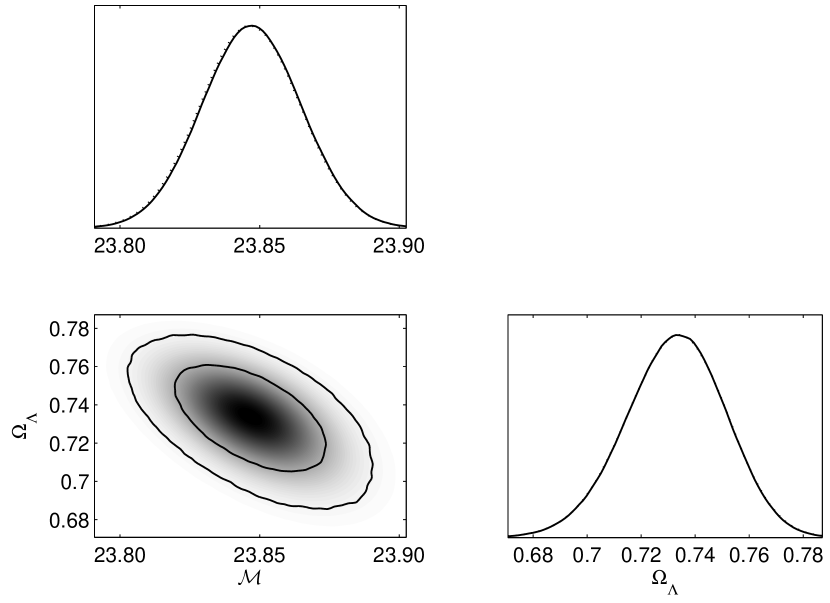
Figure 2: One and two-dimensional likelihood distributions for a cosmological constant model ($\Lambda$). Solid lines are marginalized 1D likelihoods and dotted lines mean 1D likelihoods. Solid 2D contours represent 68.3% and 95.4% regions of the marginalized distribution, and shading reflects the mean distribution.

V.1.1 Cosmological constant ($D=2$)

The probability distributions for the cosmological constant case are shown in Fig. 2. The parameter constraints in Table 2 are improved by roughly a factor of two compared to our previous analysis oldppr . They differ slightly from the results of Ref. liddledeev using the same dataset, albeit within uncertainties. This is most likely due to their different treatment of SNLS SNIa errors.

V.1.2 Skater ($D=3$)

The likelihood distributions are shown in Fig. 3 for the full dataset, and in Fig. 4 for SNLS alone. Note the symmetry in $\dot{\phi}_{0}$, due to the dependence only on $\dot{\phi}_{0}^{2}$. The degeneracy between $V_{0}$ and $\dot{\phi}_{0}$ present in our previous analysis (where $|\dot{\phi}_{0}|$ was positively correlated with $V_{0}$) is no longer apparent with the full dataset, while still being visible if we use supernovae alone. This degeneracy stems from the fact that with supernovae we are really only sensitive to an effective quintessence equation of state maordl ; maorw , which the data require to be close to $-1$. Thus, increasing the kinetic energy of the field must be compensated by an increase in potential energy to maintain the same effective equation of state.

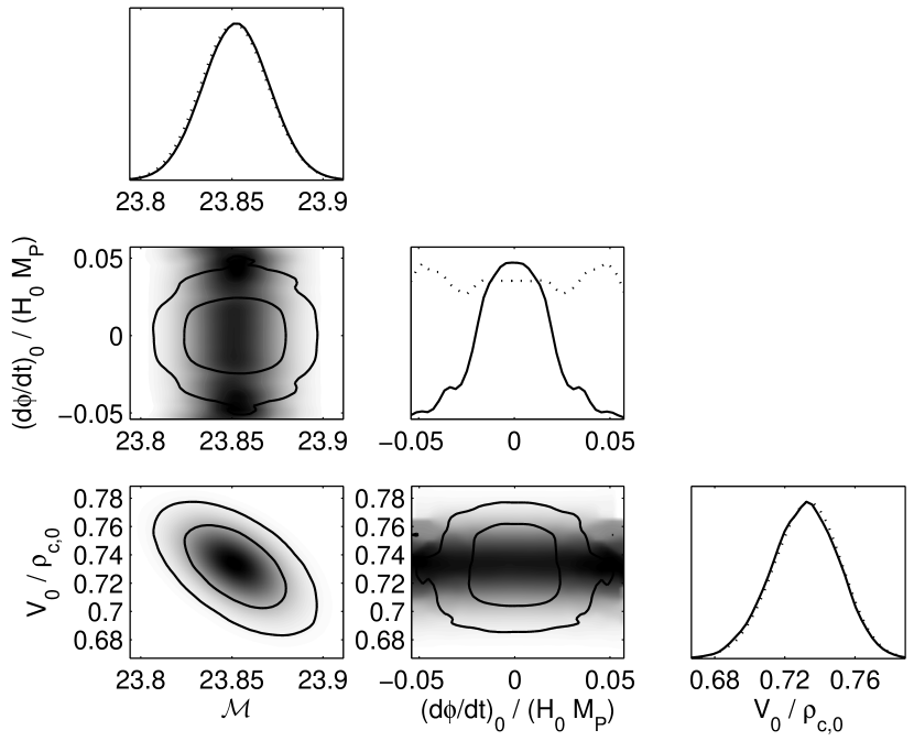
Figure 3: As Fig. 2 for a ‘skater’ model, a constant potential with kinetic energy.

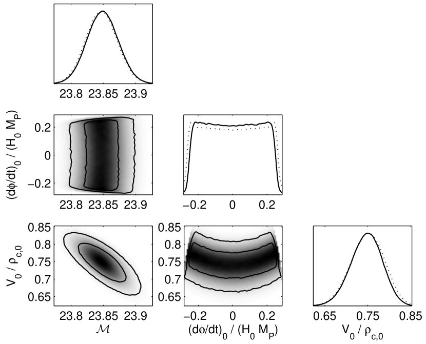
Figure 4: As Fig. 2 for a constant potential with kinetic energy. SNLS data only. Note that here the prior $\Omega_{\rm kin}(z\geq 1)<0.5$ is applied only up to $z=2$.

Additionally, the mild preference in the Riess et al. ‘gold’ data for a non-zero $\dot{\phi}_{0}$ is not present in the SNLS sample, despite the $\dot{\phi}_{0}$–$V_{0}$ degeneracy being present. Instead, the likelihood distribution is essentially flat in $\dot{\phi}_{0}$. This could be a reflection of the better quality/homogeneity of the SNLS sample over Riess et al. (another possibility is the difference in redshift coverage). In the previous analysis, these two effects conspired to give a different best-fit value of $V_{0}$ in the skater scenario ($V_{0}=0.74$) compared to the cosmological constant (where $V_{0}=\Omega_{\Lambda}=0.69$). That we here do not feel the degeneracy is to some degree linked to our prior limiting $\Omega_{\rm kin}(z\geq 1)<0.5$ now being applied to much higher redshifts, restricting the range of allowed $\dot{\phi}_{0}$. However the new data do reduce the degeneracy significantly on their own (we checked by doing the analysis without the prior on $\Omega_{\rm kin}$). Also, using only the SNLS data with $\Omega_{\rm kin}(1\leq z\leq 2)<0.5$ (Fig. 4), the flatness of the distribution in $\dot{\phi}_{0}$ ensures that the best-fit value of $V_{0}$ in that case is only marginally different from that for the full analysis, even though the degeneracy is stronger. These observations illustrate the need for good-quality data sensitive to perturbation growth history (e.g. weak lensing) to break the $\dot{\phi}_{0}$–$V_{0}$ degeneracy.

V.1.3 Linear potential ($D=4$)

The likelihood distributions are shown in Fig. 5. Note the bimodality of the $\dot{\phi}_{0}$–$V_{1}$ distribution, reflecting that models are identical under simultaneous change of sign of $\dot{\phi}_{0}$ and odd-order expansion coefficients. The first change from previous constraints oldppr is that the $V_{0}$–$\dot{\phi}_{0}$ degeneracy is now clearly visible in the case of the linear potential (there were only hints of it in the previous analysis). That is to say, the data quality is getting closer to hitting the degeneracy. In addition, we have a degeneracy between $V_{1}$ and $\dot{\phi}_{0}$, coming from the possibility to achieve a particular velocity of the field in the past by either changing the present velocity $\dot{\phi}_{0}$ or the slope $V_{1}$.

Figure 5: As Fig. 2 for a linear potential.

Although not excluding the possibility, the new data do not favour a potential where the field is rolling uphill (corresponding to the upper right-hand and lower left-hand quadrants of the $\dot{\phi}_{0}-V_{1}$ distribution). This appears to be due to the new SNLS data, which do not show a particular preference for a non-zero present field velocity, thus not pushing us into these quadrants. It would appear that the preference for an uphill rolling field found in our previous analysis oldppr was an artifact of the Riess et al. data. The observational consequences of such an uphill rolling field could be interpreted as $w<-1$ if an ‘unsuitable’ parameterization is used to fit the data maorw ; csakiwneg . It could thus be that the strong $w<-1$ preference found in the Riess et al. data (see e.g. Ref. nessperi ) is due to some systematic effect in the data, causing a preference for an uphill rolling field and also corresponding to a preference for $w<-1$ in fits of $w(z)$. This agrees with the findings of Nesseris and Perivolaropoulos nessperi , who for three different parameterizations of $w$ find that the best-fit $w(z)$ consistently does not cross the phantom divide line $w=-1$ with the SNLS dataset, but does with the Riess et al. ‘gold’ set. The analyses by Barger et al. barger , Xia et al. xia and Jassal et al. jassal lend support to this conclusion as well, as does a recent analysis by Nesseris and Perivolaropoulos nessperi2 , who however find that other cosmological data do gently favour phantom divide line crossing provided $0.2\lesssim\Omega_{\rm m}\lesssim 0.25$.

This also highlights the importance of interpreting analyses with care, as we are not probing $w(z)$ directly maordl ; maorw . This has been elaborated upon by several authors in terms of eigenmodes, either as principal components pca or weight functions wtfun .

V.1.4 Padé $R_{0/1}$ potential ($D=4$)

The likelihood distributions are shown in Fig. 6. As the $R_{0/1}$ potential is close to the linear case for small $\phi$, we can use this to compare results. That is, when $\dot{\phi}_{0}$ or $b_{1}$ (which mainly determine the field velocity) are close to zero we should expect results to compare well with the linear potential which, comparing Fig. 6 with Fig. 5, we see they do. Thus, the discussion above for the linear potential applies to this case as well. However, as we move away from $\dot{\phi}_{0}=0$ and $b_{1}=0$, we see that $b_{1}$ is limited to somewhat smaller values than for the linear case (using the relation $V_{1}\approx-a_{0}b_{1}$), while the constraints on $\dot{\phi}_{0}$ are almost identical. This indicates that data prefer not to move very far away from a linear potential. The other main feature of the likelihood distributions are bumps found in the $\dot{\phi}_{0}$–$b_{1}$ distributions. These are a feature of the likelihood distribution, but the exact size depends on our prior enforcing $\Omega_{\rm kin}(z\geq 1)<0.5$ up to high redshifts.

Padé series, by construction, have poles. One might be concerned about how this affects our results if the field reaches a pole, but the data is sufficiently constraining that the poles are effectively never felt. We tested this by doing the analysis with a prior excluding all models where a pole is reached before $z=5$, and saw no change in the results.

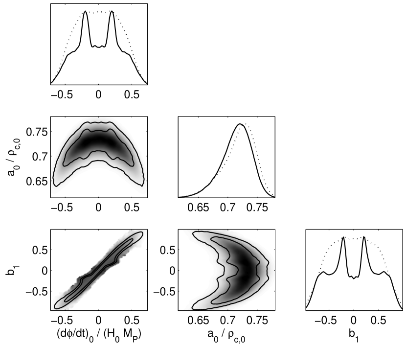
Figure 6: As Fig. 2 for a Padé series with $M=0,N=1$ ($R_{0/1}$).

	Cosmological constant $\mathbf{(\Lambda)}$	Skater	Linear	Quadratic a
$\mathcal{M}$	$23.85^{+0.02}_{-0.02}$	$23.86^{+0.01}_{-0.03}$	$23.86^{+0.02}_{-0.02}$	$23.86$
$\dot{\phi}_{0}/H_{0}M_{\rm P}$	$-$	$5.4\times 10^{-5}$ ($5.5\times 10^{-2}$) $|\dot{\phi}_{0}|/H_{0}M_{\rm P}<3.7\times 10^{-2}$ ($95\%\,{\rm CL}$)	$-2.7\times 10^{-3}$ ($-6.5\times 10^{-2}$) $|\dot{\phi}_{0}|/H_{0}M_{\rm P}<0.61$ ($95\%\,{\rm CL}$)	$-0.15$
$V_{0}/\rho_{\rm c,0}$	$0.73^{+0.02}_{-0.02}$	$0.72^{+0.03}_{-0.01}$	$0.72^{+0.02}_{-0.03}$	$0.73$
$V_{1}/\rho_{\rm c,0}$	$-$	$-$	$3.6\times 10^{-3}$ ($8.7\times 10^{-3}$) $|V_{1}|/\rho_{\rm c,0}<0.76$ ($95\%\,{\rm CL}$)	$0.58$
$V_{2}/\rho_{\rm c,0}$	$-$	$-$	$-$	$2.1$
$-2\ln{\cal L}_{\rm max}$	$113.6$	$113.4$	$113.4$	$112.9$
$\mathrm{BIC}$	$123.1$	$127.7$	$132.4$	$136.7$
$\mathrm{BIC}-\mathrm{BIC}_{\Lambda}$	$0$	$4.6$	$9.3$	$13.6$

• Since at least one parameter is unconstrained by the data for this model, we only give the best-fit parameter values found in our Markov chains.

Table 2: Marginalized median and best-fit model parameters and BIC values for the cosmological constant ($\Omega_{\Lambda}=V_{0}/\rho_{\rm c,0}$) and Taylor-series parameterizations. Best-fit values are given in parentheses when differing from the median. Note that the likelihood distribution is symmetric under simultaneous change of sign of $\dot{\phi}_{0}$ and odd-order potential expansion coefficients.

	Padé $\mathbf{R_{0/1}}$	Padé $\mathbf{R_{0/2}}$ a	Padé $\mathbf{R_{1/1}}$ a
$\mathcal{M}$	$23.86^{+0.02}_{-0.02}$	$23.86$	$23.86$
$\dot{\phi}_{0}/H_{0}M_{\rm P}$	$1.2\times 10^{-3}$ ($0.20$) $|\dot{\phi}_{0}|/H_{0}M_{\rm P}<0.57$ ($95\%\,{\rm CL}$)	$-3.9\times 10^{-2}$	$-9.8\times 10^{-2}$
$a_{0}/\rho_{\rm c,0}$	$0.72^{+0.02}_{-0.03}$	$0.73$	$0.73$
$a_{1}/\rho_{\rm c,0}$	$-$	$-$	$-0.18$
$b_{1}$	$2.1\times 10^{-3}$ ($0.18$) $|b_{1}|<0.82$ ($95\%\,{\rm CL}$)	$-0.41$	$-0.29$
$b_{2}$	$-$	$-1.2$	$-$
$-2\ln{\cal L}_{\rm max}$	$113.3$	$112.9$	$113.3$
$\mathrm{BIC}$	$132.3$	$136.7$	$137.1$
$\mathrm{BIC}-\mathrm{BIC}_{\Lambda}$	$9.2$	$13.6$	$14.0$

• See Note a of Table 2.

Table 3: Marginalized median and best-fit model parameters and BIC values for the Padé series parameterizations. Best-fit values are given in parentheses when differing from the median.

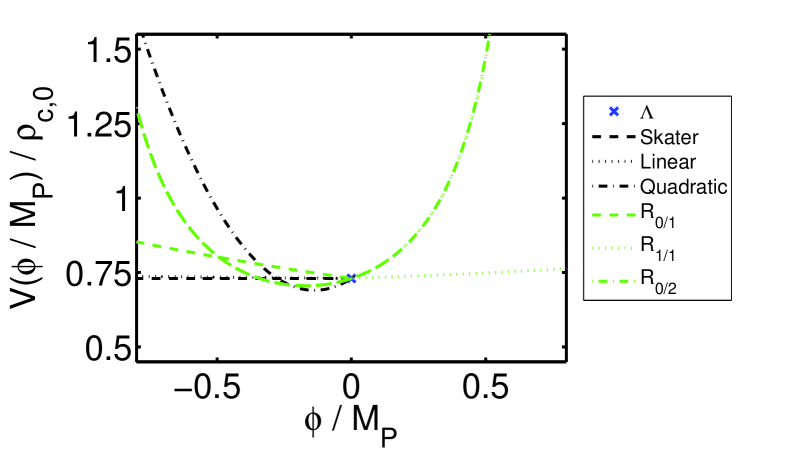
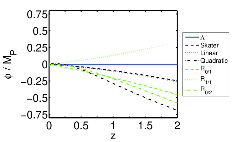
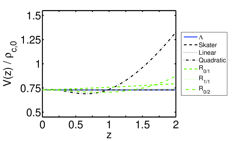
Figure 7: Best-fit potentials as a function of the field, and the field and potentials as a function of redshift.

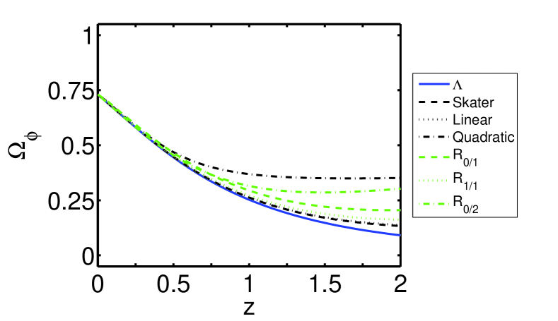
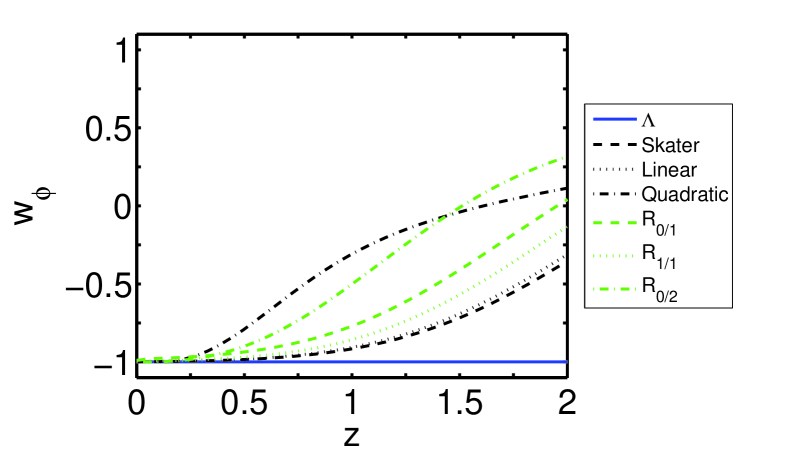
Figure 8: Best-fit $\Omega_{\phi}$ and $w_{\phi}$ as a function of redshift.

V.1.5 Models with $D>4$

In the three cases with $D=5$ (quadratic, $R_{1/1}$, and $R_{0/2}$), we find that the additional parameter is unconstrained by the data and, as in Ref. oldppr , we learn nothing useful about parameters from these models. Their principal interest lies in model comparison, discussed next, where the best-fit found can still be used to assess how the models compare in explaining the data.

V.2 Model comparison

The BIC values obtained for all models are shown in Tables 2 and 3. Note that although some parameterizations have unconstrained parameters, their BIC value can be evaluated with Eq. (37) from the best fit found in our Monte Carlo Markov chains. It is clear that the cosmological constant, showing a BIC difference of at least $4.6$ compared to the other models, is positively favoured. This is a strengthening compared to our previous analysis where this value was $4.0$. In fact, the best-fit $\chi^{2}$ changes only marginally between models, thus providing strong evidence against linear/Padé $R_{0/1}$ and higher-order potentials whose extra parameters add no value. An interesting feature of the new dataset is that it much more strongly disfavours a quadratic potential over the other Taylor expansions than just the Riess et al. data. Likewise, the lowest-order Padé expansion is favoured by the same amount compared to the higher-order Padé expansions.

The best-fit cosmologies (Figs. 7 and 8) now show more convergence in their dynamical properties, although still exhibiting increasing variation with redshift. In particular, we find that where previously the evolution of $\Omega_{\phi}$ for the best-fit quadratic potential was such that $\Omega_{\phi}$ stayed between $0.75$ and $0.96$ (for $0\leq z\leq 2$), the evolution is now very reasonable (see Fig. 8). The strong evolution previously seen in $w_{\phi}$ is now more limited, reflecting the order-of-magnitude smaller best-fit values for $\dot{\phi}_{0}$ and $V_{1}$ (though the overall compression of the uncertainties is much less than this).

All best-fit models fall into the ‘freezing’ category of Caldwell and Linder CL . For the skater model this behaviour is built-in, but it is somewhat intriguing in terms of naturalness that the best-fit linear potential exhibits freezing while at the same time rolling downhill (see Figs. 7 and 8). The potentials with curvature incorporate this best-fit behaviour by making the field reach the potential minimum in the recent past (around $z=0.5$ to $z=1$), thus providing a braking force to precipitate the accelerated expansion of the universe. This situation would appear somewhat more natural from a dynamical point of view, and it could be that the best-fit linear potential is trying to approximate this, though data is unable to sufficiently constrain the models with curvature in the potential. On the other hand, model selection using the BIC also strongly disfavours these models. The conclusion must be that complementary or better-quality data is needed to resolve this possible contradiction.

If the linear-potential results stand up, they will put the well-motivated models of quintessence based on pseudo-Nambu-Goldstone bosons (pNGBs) pngb and similar models under pressure, as these rely on a thawing field that is becoming dynamical and cosmologically dominant in the present epoch. However a field just passing the potential minimum fits well with the pNGB picture, as well as other tracker-type potentials that show a cross-over behaviour, such as the SUGRA sugra and Albrecht–Skordis AS potentials where the field is starting to feel a curvature in the potential at late times. These models exhibit early quintessence earlyquint , and can thus be constrained using big bang nucleosynthesis and CMB observations bean . It will be interesting to see what future data, including those sensitive to perturbation growth and supernovae, can tell.

These observations are in line with studies by e.g. Bludman bludman and Linder linderpaths , who both conclude that quintessence generically cannot be described by slow-roll, and that tracking must break down and move towards slow-roll in the recent past (begging the question why this is happening precisely now).

V.3 Tracker viability

In carrying out the tracker viability analysis, we consider four implementations in all by combining two choices of conditions. The first is to demand either that the field remains in the tracker regime until the present, or that it is allowed to break out of tracking after a redshift of $z=1$. The second is to consider two different upper limits for the redshift range where the field is required to be in the tracker regime, namely $z=2$ and $z=10$; the former more or less represents where the data actually lie, while the latter extrapolates the potential to higher redshifts.

We find that all four cases give qualitatively the same outcome, and so focus on just one choice, where tracking is imposed between $z=10$ and $z=1$.

The model average of $\ln B_{12}$, denoted $\langle\ln B_{12}\rangle$, for this scenario is shown in Fig. 9, for different combinations of $\epsilon$ and $\delta$. For combinations of sufficiently-small $\epsilon$ and $\delta$, no models satisfying our tracker conditions are found in the prior and/or posterior (with those $\epsilon$ and $\delta$ limits different for the different parameterizations). We exclude these cases from our model average, as they effectively correspond to an infinite uncertainty in the derived value for $\ln B_{12}$. A very small fraction of the models feel the presence of a pole at a redshift lower than the upper tracker regime redshift, and are also excluded. We also point out that for Padé $R_{0/1}$, $\Gamma=2$. Thus, the first two tracker conditions are automatically fulfilled, corresponding to a delta-function prior on $C_{1}$ and $C_{2}$ in the language of Appendix B. One might consider this a strong bias, and hence we exclude this parameterization from our Bayes factor model average, and thus use the quadratic, $R_{1/1}$ and $R_{0/2}$ potentials to arrive at our conclusions.

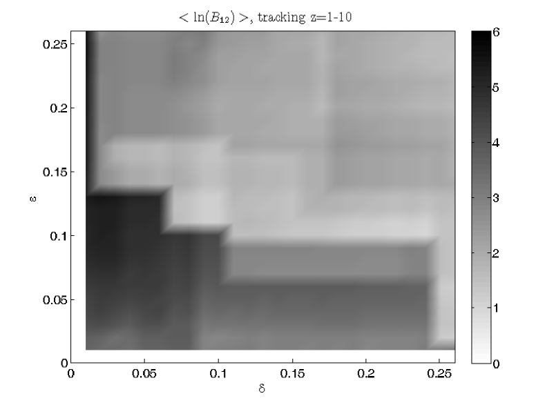
Figure 9: Model average of $\ln(B_{12})$ for tracking required between redshift 1 and 10, as a function of $\epsilon$ and $\delta$.

It is clear from Fig. 9 that the average indication is in favour of tracker behaviour over non-tracker behaviour. The smallest value of the Bayes factor in the figure is $0.98$. Limiting our attention to the region where $\epsilon\leq 0.1,\delta\leq 0.1$, and hence the tracker conditions are best obeyed, the smallest value is $2.9$. This general trend is seen in all four cases we analyze, with the strongest preference for tracking in the case presented. However, the model uncertainties in $\langle\ln B_{12}\rangle$ are comparable to $\langle\ln B_{12}\rangle$ (particularly for small $\epsilon$ and $\delta$) and a firm conclusion thus cannot be drawn. (As a side note, the Poisson uncertainties are relatively small and contribute at most on the order of $10\%$ to the total uncertainties.)

The possible preference for tracker fields is in contrast with the commonly-discussed expectation $w^{\rm eff}_{\phi}\gtrsim-0.8$ for trackers, based on general inverse-power-law series potentials steintrack (here, $w^{\rm eff}_{\phi}=\int^{1}_{a_{\rm obs}}w_{\phi}(a)\Omega_{\phi}(a){\rm d}a/\int^{1}_{a_{\rm obs}}\Omega_{\phi}(a){\rm d}a$). While this seems to indicate that tracker potentials are disfavoured by current data, our results suggest that the data may act somewhat more strongly against non-tracker models than against tracker ones.

VI Conclusions

We have updated parameter constraints on the quintessence potential along with cosmological parameters using recent SNLS supernova luminosity–redshift data, the WMAP3 CMB peak-shift parameter measurement, and the SDSS measurement of baryon oscillations. The preferred field dynamics appear robust under the different parameterizations used.

We find that, compared to our previous work oldppr , parameter constraints are improved by roughly a factor of two. We also find that linear-potential models where the field rolls uphill, although not excluded, no longer provide the best fit to the data. The previous mild preference for these models appears to have been an artifact of the Riess et al. ‘gold’ SNIa data. This observation agrees with the conclusions of other authors that the SNLS data do not particularly favour an equation of state crossing the phantom divide line, whereas the Riess et al. data do. Although higher-order potentials are not constrained by the data, those best-fit potentials exhibit ‘cross-over’ behaviour, feeling a curvature in the potential in the recent past. This qualitatively agrees with some well-motivated tracking quintessence models.

From the point of view of model selection, the cosmological constant is now even more strongly favoured compared to the dynamical models we consider (see also Refs. SWB ; liddledeev ). The models with curvature in the potential are also strongly disfavoured as compared to the constant and linear potentials, which appear dynamically less natural in the context of the complete evolution expected from high redshift.

We employ a model selection framework to investigate whether potentials that exhibit tracker behaviour at intermediate/late times are favoured by data over those potentials that do not. We conclude that although our results show some indication that tracker behaviour is favoured, the model uncertainty on the result is too large to draw any firm conclusion. We note that if the dynamics of our higher-order best-fit potentials and the preference for a tracking potential both stand up in the light of new data, the coincidence problem in the context of quintessence may simply appear in a new guise — why is the field starting to slow-roll now?

It will be interesting to see how future perturbation growth data will help break degeneracies, and, combined with supernova and CMB data, constrain quintessence models and potentially change the model selection picture as well.

Appendix A Uncertainty in tracker Bayes factor estimates

For simplicity of notation we define $E\equiv\ln B_{12}$ in this Section. The uncertainty in our estimate of $E$ will consist of two components: Poisson noise from sampling the distribution, and model uncertainty. The Poisson noise goes as

$$\sigma^{2}_{f_{\rm pri}} = f_{\rm pri}/N_{\rm pri}\,,$$ (46)

$$\sigma^{2}_{f_{\rm post}} = f_{\rm post}/N_{\rm post}\,,$$ (47)

where $N_{\rm pri}$ and $N_{\rm post}$ are the total numbers of samples drawn from the prior and posterior distribution respectively. Accordingly, using standard error propagation with Eq. (45), we have that

$$\sigma^{2}_{B_{12}}=D^{2}\sigma^{2}_{C}+C^{2}\sigma^{2}_{D}+2B_{12}{\rm cov}(C,D)\,,$$ (48)

with $C=f_{\rm post}/(1-f_{\rm post})$ and $D=(1-f_{\rm pri})/f_{\rm pri}$ so that $B_{12}=CD$. Additionally, we have

$$\sigma^{2}_{C} = \frac{\sigma^{2}_{f_{\rm post}}}{(1-f_{\rm post})^{4}}\,,$$ (49)

$$\sigma^{2}_{D} = \frac{\sigma^{2}_{f_{\rm pri}}}{f^{4}_{\rm pri}}\,.$$ (50)

In the absence of knowledge about the covariance between $C$ and $D$, we can place an upper limit on the Poisson uncertainty,

$$\sigma^{2}_{B_{12}}\leq\left(D\sigma_{C}+C\sigma_{D}\right)^{2}\,.$$ (51)

We use this upper limit as our estimate for the Poisson uncertainty. The corresponding uncertainty in $E$ is then

$$\sigma_{E} = \frac{\sigma_{C}}{C}+\frac{\sigma_{D}}{D}$$ (52)

$$= \frac{\sigma_{f_{\rm post}}}{f_{\rm post}(1-f_{\rm post})}+\frac{\sigma_{f_{\rm pri}}}{f_{\rm pri}(1-f_{\rm pri})}\,.$$

The model average of $E$ over $M$ models is given by (note that this quantity is denoted $\langle\ln B_{12}\rangle$ in the main text)

$$\bar{E}=\frac{\sum_{i}E_{i}}{M}$$ (53)

with an associated uncertainty

$$\sigma_{\bar{E}}=\sqrt{\frac{\sum_{i}(\bar{E}-E_{i})^{2}}{M(M-1)}}\,.$$ (54)

We will now have an ‘error on the error’ from the Poisson uncertainty, given by

$$\sigma_{\sigma_{\bar{E}}}=\sqrt{\frac{\sum_{i}(\bar{E}-E_{i})^{2}\sigma_{E_{i}}^{2}}{M(M-1)\sum_{i}(\bar{E}-E_{i})^{2}}}\,,$$ (55)

so our final estimate of $E$ will be

$$E = \bar{E}$$

$$\pm \left[\sqrt{\frac{\sum_{i}(\bar{E}-E_{i})^{2}}{M(M-1)}}+\sqrt{\frac{\sum_{i}(\bar{E}-E_{i})^{2}\sigma_{E_{i}}^{2}}{M(M-1)\sum_{i}(\bar{E}-E_{i})^{2}}}\right]\,.$$

Appendix B Tracker probability distributions

Here we briefly describe a possible extension of the tracker analysis carried out in this paper, though we believe application to present data would be premature.

To address the model uncertainty in the Bayes factor model average, we consider the probability distributions of the parameters that determine whether a model is classed as a tracker. In more detail, we can define three different ‘tracker functions’

$$C_{1}[\mathbf{z}_{\rm tr}] = \min_{\rm z\in\mathbf{z}_{\rm tr}}\left(\Gamma(z)-5/6\right)\,,$$ (57)

$$C_{2}[\mathbf{z}_{\rm tr}] = \max_{\rm z\in\mathbf{z}_{\rm tr}}\left|\Gamma(z)^{-1}\frac{d\Gamma(z)}{d\ln a}\right|\,,$$ (58)

$$C_{3}[\mathbf{z}_{\rm tr}] = \max_{\rm z\in\mathbf{z}_{\rm tr}}\left|w_{\phi}(z)-w_{\rm tracker}(z)\right|\,,$$ (59)

where $\mathbf{z}_{\rm tr}$ is the redshift range for which the field is required to exhibit tracker behaviour, and record their values for all elements in our MCMC chains. Note that we do not include a function corresponding to the constraint $w_{\phi}<0$, as $\max w_{\phi}(z)$ will be a function of $C_{1}$ and $C_{3}$. From this we obtain the posterior probability distribution $P(C_{1},C_{2},C_{3}|\Pi(\mathbf{\Theta}))$ given the prior distribution $\Pi(\mathbf{\Theta})$ for our primary cosmological parameters $\mathbf{\Theta}$. Running the MCMC for the prior distribution as well, we obtain the prior distribution $\Pi(C_{1},C_{2},C_{3}|\Pi(\mathbf{\Theta}))$.

We are then in a position to do importance sampling (see e.g. Appendix B in Ref. Lewis:2002ah for a brief introduction) using the prior and posterior we have calculated. We can change priors for $C_{1},C_{2},C_{3}$ from those induced by $\Pi(\mathbf{\Theta})$ to whichever we like and obtain the corresponding new posterior distribution, since we only need to divide out the prior distribution and multiply by the prior of our choice (with the exception of parts of parameter space cut out by the primary prior $\Pi(\mathbf{\Theta})$ or very poorly sampled). A potential problem with this approach is that optimal sampling of the posterior distribution in $C_{1},C_{2},C_{3}$ is not necessarily achieved by optimal sampling in the primary parameters, and sufficient statistics may take a long time, i.e. many chain elements, to accumulate.

Setting natural priors for these new parameters may be perceived as difficult (although not manifestly more arbitrary than for other phenomenological parameterizations). A simple way of setting the priors is to argue that we should be equally likely to draw a parameter value that fulfils the corresponding tracker criterion, as one that doesn’t. For instance, if we assume Gaussian priors, we get

$$P(C_{1}) = \frac{1}{\sqrt{2\pi}\sigma_{C_{1}}}\exp\left[-\frac{C_{1}^{2}}{2\sigma^{2}_{C_{1}}}\right]\,,$$ (60)

$$P(C_{2}) = \frac{2}{\sqrt{2\pi}\sigma_{C_{2}}}\exp\left[-\frac{C_{2}^{2}}{2\sigma^{2}_{C_{2}}}\right]\theta(C_{2})\,,$$ (61)

$$P(C_{3}) = \frac{2}{\sqrt{2\pi}\sigma_{C_{3}}}\exp\left[-\frac{C_{3}^{2}}{2\sigma^{2}_{C_{3}}}\right]\theta(C_{3})\,,$$ (62)

where $\theta$ is the Heaviside step function ($C_{2}$ and $C_{3}$ are restricted to non-negative values by definition). The standard deviations $\sigma_{C_{2}}$ and $\sigma_{C_{3}}$ are set by then demanding

$$\int_{C_{2}\leq\epsilon}P(C_{2}){\rm d}C_{2} = \int_{C_{2}>\epsilon}P(C_{2}){\rm d}C_{2}\,,$$ (63)

$$\int_{C_{3}\leq\delta}P(C_{3}){\rm d}C_{3} = \int_{C_{3}>\delta}P(C_{3}){\rm d}C_{3}\,.$$ (64)

The case of $C_{1}$ is different, since we only have one inequality to fulfil ($\Gamma>5/6$). Hence, we need to put a cut-off at some value to determine the standard deviation. One could of course assign, for example, flat priors in the same fashion.

Using this method, we can thus obtain a posterior distribution $P(C_{1},C_{2},C_{3})$ for a given prior distribution $\Pi(C_{1},C_{2},C_{3})$ of our choice, thus allowing a removal of correlation biases intrinsic to particular parameterizations, which should reduce model uncertainty. This method allows us to perform parameter estimation on $C_{1},C_{2},C_{3}$ as well as model selection by calculating the Bayesian evidence. It is of course applicable to general dynamical cosmological properties one might wish to study. Carrying this out in practice can however be involved since we might not be sampling efficiently in the MCMC, and performing model selection in a robust manner would require specialized code to address the sampling inefficiency and to handle the use of a binned distribution.

References

- (1) A. Albrecht et al. (Dark Energy Task Force report), astro-ph/0609591.
- (2) C. Wetterich, Nucl. Phys. B302, 668 (1988); B. Ratra and P. J. E. Peebles, Phys. Rev. D37, 3406 (1988).
- (3) V. Sahni and A. A. Starobinsky, Int. J. Mod. Phys. D9, 373 (2000), astro-ph/9904398; S. M. Carroll, Living Rev. Rel. 4, 1 (2001); T. Padmanabhan, Phys. Rept. 380, 235 (2003), hep-th/0212290; V. Sahni, Class. Quant. Grav. 19, 3435 (2002); T. Padmanabhan, Phys. Rept. 380, 235 (2003); P. J. E. Peebles and B. Ratra, Rev. Mod. Phys. 75, 559 (2003); E. J. Copeland, M. Sami, and S. Tsujikawa (2006), hep-th/0603057; V. Sahni and A. Starobinsky, astro-ph/0610026.
- (4) D. Huterer and M. S. Turner, Phys. Rev. D60, 081301(R) (1999), astro-ph/9808133; A. A. Starobinsky, JETP Lett. 68, 757 (1998) [Pisma Zh. Eksp. Teor. Fiz. 68, 721 (1998)], astro-ph/9810431; T. Nakamura and T. Chiba, Mon. Not. Roy. Astron. Soc. 306, 696 (1999), astro-ph/9810447; T. D. Saini, S. Raychaudhury, V. Sahni, and A. A. Starobinsky, Phys. Rev. Lett. 85, 1162 (2000), astro-ph/9910231; B. F. Gerke and G. Efstathiou, Mon. Not. Roy. Astron. Soc. 335, 33 (2002), astro-ph/0201336; C. Wetterich, Phys. Lett. B594, 17 (2004), astro-ph/0403289; J. Simon, L. Verde, and R. Jimenez, Phys. Rev. D71, 123001 (2005), astro-ph/0412269; Z. K. Guo, N. Ohta, and Y. Z. Zhang, Phys. Rev. D72, 023504 (2005), astro-ph/0505253; S. Tsujikawa, Phys. Rev. D72, 083512 (2005), astro-ph/0508542; Z. K. Guo, N. Ohta, and Y. Z. Zhang, astro-ph/0603109; X. Zhang, Phys. Rev. D74, 103505 (2006), astro-ph/0609699.
- (5) R. A. Daly and S. G. Djorgovski, Astrophys. J. 597, 9 (2003), astro-ph/0305197; R. A. Daly and S. G. Djorgovski, Astrophys. J. 612, 652 (2004), astro-ph/0403664; R. A. Daly and S. G. Djorgovski, astro-ph/0512576; R. A. Daly and S. G. Djorgovski, astro-ph/0609791.
- (6) M. Sahlén, A. R. Liddle, and D. Parkinson, Phys. Rev. D72, 083511 (2005), astro-ph/0506696.
- (7) A. G. Riess et al. [Supernova Search Team Collaboration], Astrophys. J. 607, 665 (2004), astro-ph/0402512.
- (8) D. N. Spergel et al. [WMAP collaboration], astro-ph/0603449.
- (9) D. J. Eisenstein et al. [SDSS Collaboration], Astrophys. J. 633, 560 (2005), astro-ph/0501171.
- (10) P. Astier et al., Astron. Astrophys. 447, 31 (2006), astro-ph/0510447.
- (11) D. Huterer and H. V. Peiris, astro-ph/0610427.
- (12) R. R. Caldwell and E. V. Linder, Phys. Rev. Lett. 95, 141301 (2005), astro-ph/0505494.
- (13) E. V. Linder, Astropart. Phys. 24, 391 (2005), astro-ph/0508333.
- (14) G. A. Baker and P. R. Graves-Morris, Padé Approximants, Vol. 1 & 2, Addison-Wesley (1981).
- (15) E. V. Linder and D. Huterer, Phys. Rev. D72, 043509 (2005), astro-ph/0505330.
- (16) I. Maor and R. Brustein, Phys. Rev. D67, 103508 (2003), hep-ph/0209203.
- (17) P. G. Ferreira and M. Joyce, Phys. Rev. Lett. 79, 4740 (1997), astro-ph/9707286; E. J. Copeland, A. R. Liddle, and D. Wands, Phys. Rev. D57, 4686 (1998), gr-qc/9711068; P. G. Ferreira and M. Joyce, Phys. Rev. D58, 023503 (1998), astro-ph/9711102; I. Zlatev, L. Wang, and P. J. Steinhardt, Phys. Rev. Lett. 82, 896 (1999), astro-ph/9807002; A. R. Liddle and R. J. Scherrer, Phys. Rev. D59, 023509 (1998), astro-ph/9809272; I. Zlatev and P. J. Steinhardt, Phys. Lett. B 459, 570 (1999), astro-ph/9906481; R. de Ritis, A. A. Marino, C. Rubano, and P. Scudellaro, Phys. Rev. D62, 043506 (2000), hep-th/9907198; T. Barreiro, E. J. Copeland, and N. J. Nunes, Phys. Rev. D61, 127301 (2000), astro-ph/9910214; P. Brax and J. Martin, astro-ph/9912005; L. A. Urena-Lopez and T. Matos, Phys. Rev. D62, 081302 (2000), astro-ph/0003364; V. B. Johri, Phys. Rev. D63, 103504 (2001), astro-ph/0005608; R. Bean, S. H. Hansen, and A. Melchiorri, Phys. Rev. D64, 103508 (2001), astro-ph/0104162; C. Rubano and J. D. Barrow, Phys. Rev. D64, 127301 (2001), gr-qc/0105037; V. B. Johri, Class. Quant. Grav. 19, 5959 (2002) astro-ph/0108247; C. Baccigalupi, A. Balbi, S. Matarrese, F. Perrotta, and N. Vittorio, Phys. Rev. D65, 063520 (2002), astro-ph/0109097; W. Wang and B. Feng, Chin. J. Astron. Astrophys. 3, 105 (2003), astro-ph/0508139; S. Tsujikawa, Phys. Rev. D73, 103504 (2006), hep-th/0601178; L. Amendola, M. Quartin, S. Tsujikawa, and I. Waga, Phys. Rev. D74, 023525 (2006), astro-ph/0605488; R. Das, T. W. Kephart, and R. J. Scherrer, gr-qc/0609014.
- (18) P. J. Steinhardt, L. Wang, and I. Zlatev, Phys. Rev. D59, 123504 (1999), astro-ph/9812313.
- (19) S. Bludman, Phys. Rev. D69, 122002 (2004), astro-ph/0403526.
- (20) E. V. Linder, Phys. Rev. D73, 063010 (2006), astro-ph/0601052.
- (21) Y. Wang, J. M. Kratochvil, A. Linde, and M. Shmakova, JCAP 0412, 006 (2004), astro-ph/0409264.
- (22) D. Fouchez, priv. comm.
- (23) J. R. Bond, G. Efstathiou, and M. Tegmark, Mon. Not. Roy. Astron. Soc. 291, L33 (1997), astro-ph/9702100; M. Zaldarriaga, D. N. Spergel, and U. Seljak, Astrophys. J. 488, 1 (1997), astro-ph/9702157; G. Efstathiou and J. R. Bond, Mon. Not. Roy. Astron. Soc. 304, 75 (1999), astro-ph/9807103.
- (24) Y. Wang and P. Mukherjee, Astrophys. J 650, 1 (2006), astro-ph/0604051.
- (25) D. J. Eisenstein and W. Hu, Astrophys. J. 496, 605 (1998), astro-ph/9709112; C. Blake and K. Glazebrook, Astrophys. J. 594, 665 (2003), astro-ph/0301632.
- (26) S. Cole et al. [The 2dFGRS Collaboration], Mon. Not. Roy. Astron. Soc. 362, 505 (2005), astro-ph/0501174.
- (27) G. Schwarz, Annals of Statistics 5, 461 (1978).
- (28) A. R. Liddle, Mon. Not. Roy. Astron. Soc. 351, L49 (2004), astro-ph/0401198.
- (29) H. Jeffreys, Theory of Probability, 3rd ed., Oxford University Press (1961).
- (30) S. Mukherjee, E. D. Feigelson, G. J. Babu, F. Murtagh, C. Fraley, and A. Raftery, Astrophys. J. 508, 314 (1998), astro-ph/9802085.
- (31) B. A. Bassett, P. S. Corasaniti, and M. Kunz, Astrophys. J. Lett. 617, L1 (2004), astro-ph/0407364; M. Szydlowski and W. Godlowski, Phys. Lett. B633, 427 (2006); M. Szydlowski, A. Kurek, and A. Krawiec, Phys. Lett. B642, 171 (2006), astro-ph/0604327.
- (32) R. E. Kass and A. E. Raftery, Journal of the American Statistical Association 90, 773 (1995); R. Trotta, astro-ph/0504022; P. Mukherjee, D. Parkinson, P. S. Corasaniti, A. R. Liddle, and M. Kunz, Mon. Not. Roy. Astron. Soc. 369, 1725 (2006), astro-ph/0512484; A. R. Liddle, P. Mukherjee, and D. Parkinson, astro-ph/0608184.
- (33) A. R. Liddle, P. Mukherjee, D. Parkinson, and Y. Wang, Phys. Rev. D74, 123506 (2006), astro-ph/0610126.
- (34) I. Maor, R. Brustein, J. McMahon, and P. J. Steinhardt, Phys. Rev. D65, 123003 (2002), astro-ph/0112526.
- (35) I. Maor, R. Brustein and P. J. Steinhardt, Phys. Rev. Lett. 86, 6 (2001) [Erratum-ibid. 87, 049901 (2001)], astro-ph/0007297.
- (36) C. Csaki, N. Kaloper, and J. Terning, JCAP 0606, 022 (2006), astro-ph/0507148.
- (37) S. Nesseris and L. Perivolaropoulos, Phys. Rev. D72, 123519 (2005), astro-ph/0511040.
- (38) V. Barger, E. Guarnaccia, and D. Marfatia, Phys. Lett. B 635, 61 (2006), hep-ph/0512320.
- (39) J. Q. Xia, G. B. Zhao, B. Feng, H. Li, and X. Zhang, Phys. Rev. D73, 063521 (2006), astro-ph/0511625.
- (40) H. K. Jassal, J. S. Bagla, and T. Padmanabhan, astro-ph/0601389.
- (41) S. Nesseris and L. Perivolaropoulos, astro-ph/0610092.
- (42) D. Huterer and G. Starkman, Phys. Rev. Lett. 90, 031301 (2003), astro-ph/0207517; D. Huterer and A. Cooray, Phys. Rev. D71, 023506 (2005), astro-ph/0404062; R. G. Crittenden and L. Pogosian, astro-ph/0510293; C. Stephan-Otto, Phys. Rev. D74, 023507 (2006), astro-ph/0605403.
- (43) T. D. Saini, T. Padmanabhan, and S. Bridle, Mon. Not. Roy. Astron. Soc. 343, 533 (2003), astro-ph/0301536; T. D. Saini, Mon. Not. Roy. Astron. Soc. 344, 129 (2003), astro-ph/0302291; F. Simpson and S. Bridle, Phys. Rev. D71, 083501 (2005), astro-ph/0411673; F. Simpson and S. Bridle, Phys. Rev. D73, 083001 (2006), astro-ph/0602213.
- (44) C. T. Hill, D. N. Schramm, and J. N. Fry, Comments Nucl. Part. Phys. 19, 25 (1989); J. A. Frieman, C. T. Hill, and R. Watkins, Phys. Rev. D46, 1226 (1992); M. Fukugita and T. Yanagida, YITP-K-1098 (1994); J. A. Frieman, C. T. Hill, A. Stebbins, and I. Waga, Phys. Rev. Lett. 75, 2077 (1995), astro-ph/9505060; N. Kaloper and L. Sorbo, JCAP 0604, 007 (2006), astro-ph/0511543.
- (45) P. Binetruy, Phys. Rev. D60, 063502 (1999), hep-ph/9810553; P. Brax and J. Martin, Phys. Lett. B468, 40 (1999), astro-ph/9905040; P. Brax, J. Martin and A. Riazuelo, Phys. Rev. D64, 083505 (2001), hep-ph/0104240.
- (46) A. Albrecht and C. Skordis, Phys. Rev. Lett. 84, 2076 (2000), astro-ph/9908085; C. Skordis and A. Albrecht, Phys. Rev. D66, 043523 (2002), astro-ph/0012195.
- (47) C. Wetterich, JCAP 0310, 002 (2003), hep-ph/0203266; C. Wetterich, Phys. Lett. B561, 10 (2003), hep-ph/0301261; R. R. Caldwell, M. Doran, C. M. Mueller, G. Schaefer, and C. Wetterich, Astrophys. J. 591, L75 (2003), astro-ph/0302505; M. Doran and G. Robbers, JCAP 0606, 026 (2006), astro-ph/0601544.
- (48) R. Bean, S. H. Hansen, and A. Melchiorri, Phys. Rev. D64, 103508 (2001), astro-ph/0104162.
- (49) T. D. Saini, J. Weller, and S. L. Bridle, Mon. Not. Roy. Astron. Soc. 348, 603 (2004), astro-ph/0305526.
- (50) A. Lewis and S. Bridle, Phys. Rev. D66, 103511 (2002), astro-ph/0205436.