High Resolution Submillimeter Constraints on Circumstellar Disk Structure

Abstract

We present a high spatial resolution submillimeter continuum survey of 24 circumstellar disks in the Taurus-Auriga and Ophiuchus-Scorpius star formation regions using the SMA. In the context of a simple model, we use broadband spectral energy distributions and submillimeter visibilities to derive constraints on some basic parameters that describe the structure of these disks. For the typical disk in the sample we infer a radial surface density distribution $\Sigma_{r}\propto r^{-p}$ with a median $p\approx 0.5$, although consideration of the systematic effects of some of our assumptions suggest that steeper distributions with $p\approx 0.7-1.0$ are more reasonable. The distribution of the outer radii of these disks shows a distinct peak at $R_{d}\approx 200$ AU, with only a few cases where the disk emission is completely unresolved. Based on these disk structure measurements, the mass accretion rates, and the typical spectral and spatial distributions of submillimeter emission, we show that the observations are in good agreement with similarity solutions for steady accretion disks that have a viscosity parameter $\alpha\approx 0.01$. We provide new estimates of the spectral dependence of the disk opacity $\kappa_{\nu}\propto\nu^{\beta}$ with a median $\beta\approx 0.7$, corrected for optically thick emission. This typical value of $\beta$ is consistent with model predictions for the collisional growth of solids to millimeter size scales in the outer disk. Although direct constraints on planet formation in these disks are not currently available, the extrapolated density distributions inferred here are substantially shallower than those calculated based on the solar system or extrasolar planets and typically used in planet formation models. It is possible that we are substantially underestimating disk densities due to an incomplete submillimeter opacity prescription.

1 Introduction

Circumstellar disks play integral roles in early stellar evolution and the genesis of planetary systems. As the gas and dust reservoirs that contain the raw material for building planets, these disks provide a snapshot of the planet formation process. Any model of this process is necessarily dependent on the distribution and composition of the progenitor disk material (e.g., Pollack et al., 1996; Inaba et al., 2003; Boss, 2005; Durisen et al., 2005). In principle, observations related to the structure and content of these disks can be used to constrain the timescales and mechanisms involved in building planets. Key insights into the origins of planetary systems can also be determined based on the dynamical and physical properties of extrasolar planets (e.g., Marcy et al., 2000; Udry et al., 2006) and their host stars (Santos et al., 2001; Fischer & Valenti, 2005), as well as via the internal structure and composition of the giant planets (Lunine et al., 2004; Guillot, 2005) and various aspects of the populations of smaller bodies (e.g., Luu & Jewitt, 2002) in the solar system. Studies of the ancestral circumstellar disks and their descendent planetary systems approach the topic of planet formation from opposite directions in time.

Observations that are sensitive to the structure of disks are also useful for constraining the internal mechanisms that govern their evolution. For example, the spatial density distribution and size of a disk can be combined with the mass accretion rate onto the central star (e.g., Valenti et al., 1993; Hartigan et al., 1995; Gullbring et al., 1998; Muzerolle et al., 2003a) to estimate the disk viscosity (e.g., Hartmann et al., 1998). This viscosity is thought to be generated by the magnetorotational instability (Balbus & Hawley, 1991, but see Hartmann et al. 2006) and, along with gravity and the conservation of angular momentum, dictates the structural evolution of disk material (Lynden-Bell & Pringle, 1974; Lin & Bodenheimer, 1982; Hartmann et al., 1998; Hueso & Guillot, 2005). As a second example, the spectral dependence of the disk opacity can be used to estimate the size distribution of solid particles in the disk, thereby tracing the growth of dust grains to the earliest planetesimals (Miyake & Nakagawa, 1993; D’Alessio et al., 2001, 2006; Draine, 2006). This collisional agglomeration of disk material plays a critical role in both the evolution of the disk and the planet formation process.

While there is clearly significant motivation to study the physical structure of circumstellar disks, interpreting the observational data in this context is a challenge. The focus of this paper is on observations of continuum emission from these disks, particularly at submillimeter wavelengths. This thermal emission is reprocessed starlight from irradiated dust grains. The spectral energy distribution (SED) of this emission is determined by a range of disk radii which have different temperature and density conditions. As a consequence, submillimeter continuum observations play an important role in constraining disk structure properties for three primary reasons. First, the great majority of the mass and volume of a typical disk (with radius $\gtrsim$ 100 AU) will be relatively cold, therefore emitting the bulk of the continuum at these wavelengths. Second, there should be substantial submillimeter emission in the extended outer regions of a disk, making spatially resolved observations with an interferometer possible. And third, much of the submillimeter emission is thought to be optically thin (e.g., Beckwith et al., 1990), meaning measurements of its spatial and spectral distributions can be used to readily infer the mass distribution and opacity in the disk.

The pioneering high resolution observations of submillimeter continuum emission from circumstellar disks were directed at measuring their sizes and orientations (e.g., Keene & Masson, 1990; Lay et al., 1994). As the technology and data quality improved, focus shifted to exploring the radial structure of a few resolved disks (e.g., HL Tau; Mundy et al., 1996; Wilner et al., 1996), and then in particular to determining constraints on their sizes and density distributions (e.g., Dutrey et al., 1996; Lay et al., 1997; Akeson et al., 1998, 2002; Wilner et al., 2000; Kitamura et al., 2002). A set of complementary studies used spatially resolved line emission from molecular gas phase tracers like CO to work toward the same end (e.g., Dutrey et al., 1998; Guilloteau & Dutrey, 1998; Guilloteau et al., 1999). More recently, a few of these disks have been examined under the auspices of more sophisticated models (Dutrey et al., 1998; D’Alessio et al., 2001; Calvet et al., 2002; Dartois et al., 2003) to place ever more detailed constraints on properties like structure and chemistry (Wilner et al., 2003; Qi et al., 2003, 2004, 2006; Dutrey et al., 2006), as well as the signatures of grain growth (e.g., Wilner et al., 2005).

In this paper, we utilize a survey of high spatial resolution submillimeter continuum observations and a simple model to place constraints on the physical structure of circumstellar disks. Measurements of molecular line emission (rotational transitions of CO) from these same data will be presented in a separate paper. The observations, data reduction, and basic sample properties are introduced in §2. The modeling procedure is described in detail in §3, and basic constraints on disk structure parameters are given in §4. A discussion in §5 aims to synthesize the results in the contexts of disk evolution and planet formation, with some comments on the prospects for future work on this topic. The Appendix contains additional comments on individual disks in the sample.

2 Observations and Data Reduction

Interferometric observations of 24 young star/disk systems were conducted with the Submillimeter Array (SMA; Ho et al., 2004) on the summit of Mauna Kea, Hawaii. The SMA consists of eight 6 m antennas which can be placed on 24 pads across a relatively flat valley at an altitude of $\sim$4070 m. All targets were observed in one of two different compact array configurations with baselines up to $\sim$150 m (the “C1” configuration, used before 2005 May) or $\sim$70 m (the “C2” configuration, used after 2005 May). Many of the targets were also observed in an extended (E) configuration of the array with maximum baseline lengths of $\sim$200 m.

Double sideband receivers were tuned to an intermediate frequency (IF) of either 225.494, 340.758, or 349.930 GHz (1330, 880, or 857 $\mu$m, respectively). Each sideband provides 2 GHz of bandwidth, centered $\pm 5$ GHz from the IF. The standard correlator setup adopted in this survey provides 24 partially overlapping basebands of 104 MHz width in each sideband, with a 0.8125 MHz channel spacing in each baseband. The highest frequency observations ($\nu_{\rm{IF}}=349.930$ GHz) used a slightly different correlator setup to accomodate higher spectral resolution in some basebands, leading to a slightly reduced total continuum bandwidth.

Most of the observations interleaved two targets and two quasars (complex gain calibrators) in an alternating pattern, with 20 minutes on a target and then 10 minutes on a quasar. Additional calibrators were observed at the beginning and end of a night. The quasars used for complex gain calibration were 3C 111 and 3C 84 for Taurus-Auriga targets, and J1733$-$130 and J1743$-$038 or J1517$-$243 and J1626$-$298 for Ophiuchus-Scorpius targets. Planets (Uranus, Jupiter, Saturn), satellites (Titan, Callisto), and quasars (3C 454.3, 3C 273, 3C 279) were observed as passband and absolute flux calibrators depending on their availability and the array configuration. Observing conditions were generally excellent. Data were obtained with $\lesssim$1.2 and 3 mm of precipitable water vapor for high and low frequencies, respectively, with system temperatures in the range of 100$-$400 K. A summary of basic observational information is given in Table 1.

The data were edited and calibrated using MIR, an IDL-based software package originally developed for the OVRO array and adapted by the SMA group. After appropriate editing, calibration of the passband response for each baseband was determined using a bright planet or quasar. Broadband continuum channels in each sideband were generated by averaging the central 82 MHz in all line-free basebands. The baseline-based complex gain response of the system was calibrated using one or both of the quasars interleaved with the targets. Absolute flux calibration was performed based on either planets/satellites (Uranus, Titan, or Callisto) and/or routinely-monitored quasars (e.g., 3C 454.3). Typical systematic uncertainties in the absolute flux scale of $\sim$10$-$15% were determined based both on the uncertainties of the planetary emission models or quasar flux densities and the level of agreement between various methods of performing the calibrations (data from 2004 had absolute flux calibration uncertainties at the $\sim$20% level).

The standard tasks of Fourier inversion, deconvolution with the CLEAN algorithm, and restoration with the synthesized beam were conducted with the MIRIAD software package. All continuum maps were created with natural weighting in the Fourier plane. Synthesized beam parameters are given in Table 1. Maps of the gain calibrators were checked against one another to determine the effects of pointing errors, seeing, and any small baseline errors. In general, these effects lead to positional uncertainties on the order of 0$\farcs$1 or less, with observations in 2004 slightly worse. The J2000 phase center coordinates were chosen to coincide with the stellar positions, determined from the Two Micron All-Sky Survey (2MASS) Point Source Catalog astrometry (Cutri et al., 2003).

Continuum emission maps of the sample objects are shown in Figures 1 and 2. The axes mark offsets in arcseconds, and the synthesized beam size and shape are shown in the lower left corner of each panel. Continuum flux densities for each source were determined by summing the emission within the 2 $\sigma$ contour, with the rms noise determined in an emission-free box within $\pm$20″ from the phase center. The continuum flux densities and statistical errors are listed in Table 2, along with FWHM source dimensions and orientations determined from elliptical Gaussian fits to the visibilities. Maps of multiple star systems have individual stellar positions marked with crosses, with the component exhibiting continuum emission clearly labeled in Table 2 and Figures 1$-$2. In most cases, the interferometer has recovered all of the continuum flux observed with single-dish data (Beckwith et al., 1990; André & Montmerle, 1994; Nürnberger et al., 1998; Andrews & Williams, 2005). Several of the sources, particularly those in the Ophiuchus clouds, have SMA flux densities lower than those determined with a single-dish telescope. Presumably the interferometric fluxes are lower due to the spatial filtering of extended cloud/envelope emission in these cases (see the Appendix).

The targets for this study were selected primarily by their single-dish submillimeter flux densities to ensure fairly high signal-to-noise ratios for the developing SMA. This criterion introduces a significant bias to the sample, as the brightest submillimeter disks are not necessarily representative. The median 850 $\mu$m flux density for a disk in the sample of Andrews & Williams (2005) is several times smaller than the SMA sample median. The sample is split evenly among disks in the Taurus-Auriga complex ($d\approx 140$ pc; Elias, 1978) and the Ophiuchus-Scorpius region ($d\approx 160$ pc; de Geus et al., 1989). Despite the limitations of the primary selection criterion, we attempted to compose a sample with a wide range of stellar and disk properties. The stars in the sample basically span the T Tauri spectral type range, from early G to middle M types (corresponding to $M_{*}\approx 0.1-2$ M_⊙), while the disks exhibit a broad scope of the standard characteristics attributed to accretion and/or excess photospheric emission. A significant fraction of the sample targets ($\sim$20%; 5/24) are known multiple star systems. Some basic properties of the targets are compiled in Table 3.

3 Models and Disk Structure Constraints

The spatial distribution and SED of thermal continuum emission are the primary data available for determining the structural properties of circumstellar dust disks. Reasonable estimates of the radial temperature distribution and total disk mass can be made from the mid-infrared SED and submillimeter photometry, respectively (e.g., Beckwith et al., 1990; Andrews & Williams, 2005). However, it is not possible to place constraints on either the density distribution or size of a disk without spatially resolved data. In principle, the combination of a complete SED and a spatially resolved image can be used to determine these parameters with a direct fit to a disk model.

One simple case is the “flat” disk model, which allows for a continuous radial distribution of material with power-law forms for the temperature and surface density (Adams et al., 1987). This model is able to reproduce the SEDs and submillimeter images of typical circumstellar disks quite well, and serves as a reasonable approximation for the more detailed structure of a realistic accretion disk. More sophisticated models have been advanced to address the observational and theoretical shortcomings of this model (for reviews, see Dullemond et al., 2006; Dutrey et al., 2006). For example, a disk subject to hydrostatic equilibrium in the vertical direction is flared, and therefore has an increased illuminated surface area at radii corresponding to temperatures that produce mid- and far-infrared emission (Kenyon & Hartmann, 1987; Chiang & Goldreich, 1997, 1999; Dullemond et al., 2002). However, because most of the submillimeter emission is generated near the midplane of the disk, this vertical flaring does not have a strong effect on the emission at those wavelengths (e.g., Chiang & Goldreich, 1997). While these more complex models illuminate key properties of disks, the computing power required to estimate their parameters with a minimization technique can be formidable. Based on this fact and the size and quality of the sample presented here, we focus on interpreting these data in terms of the comparatively simple flat disk description.

3.1 The Flat Disk Model

In the flat disk model, photospheric excess emission is generated by thermal reprocessing of starlight by a geometrically thin dust disk with radial temperature ($T_{r}$) and surface density ($\Sigma_{r}$) profiles described by power-laws:

$$T_{r}=T_{1}\left(\frac{r}{1\,\rm{AU}}\right)^{-q}$$ (1)

$$\Sigma_{r}=\Sigma_{5}\left(\frac{r}{5\,\rm{AU}}\right)^{-p}$$ (2)

where $T_{1}$ is the temperature at 1 AU and $\Sigma_{5}$ is the surface density at 5 AU (the normalization of $\Sigma_{r}$ is selected for comparison to Jupiter). By further assuming an opacity spectrum that is a power-law in frequency and independent of radius,

$$\kappa_{\nu}=\kappa_{0}\left(\frac{\nu}{\nu_{0}}\right)^{\beta},$$ (3)

the flux density ($F_{\nu}$) at any frequency can be determined by summing the thermal emission from annuli weighted by the optical depth ($\tau_{\nu,r}=\kappa_{\nu}\Sigma_{r}$),

$$F_{\nu}=\frac{\cos{i}}{d^{2}}\int^{R_{d}}_{r_{0}}B_{\nu}(T_{r})(1-e^{-\tau_{\nu,r}\sec{i}})\,2\pi r\,dr$$ (4)

where $i$ is the disk inclination angle (90° is edge-on), $d$ is the distance, $r_{0}$ and $R_{d}$ are the inner and outer disk edges, respectively, and $B_{\nu}(T_{r})$ is the Planck function at the given radial temperature. This model is completely described by a set of 9 parameters, {$i$, $r_{0}$, $R_{d}$, $\kappa_{0}$, $\beta$, $T_{1}$, $q$, $\Sigma_{5}$, $p$}.

With only the unresolved SED, it is not possible to uniquely determine most of these parameters (Thamm et al., 1994, see also Chiang et al. 2001 for a similar discussion with more sophisticated models). In light of this fact, the standard adopted procedure is to fix a subset of the parameters based on reasonable assumptions, usually {$i$, $r_{0}$, $R_{d}$, $\kappa_{0}$, $\beta$, $p$}, and fit to the data to determine the others (e.g., Beckwith et al., 1990; Andrews & Williams, 2005). However, when information about the spatial distribution of emission at one or more frequencies becomes available, some of the inherent parameter degeneracies can be broken. The flat disk model can be easily adapted to generate two-dimensional images at the expense of introducing the disk orientation, or position angle (PA), as an additional parameter.

3.2 Fitting Methodology and Data

To estimate flat disk model parameters for this sample, we adopt a minimization technique that simultaneously fits both the SED and the spatial distribution of continuum emission at one submillimeter wavelength. The latter is treated in the Fourier plane to avoid the nonlinearities associated with deconvolution and to properly account for the spatial response of the interferometer. To further simplify and expedite the process computationally, we utilize the circular symmetry of the flat disk model (after accounting for inclination and orientation effects) to represent the spatial distribution of emission via the one-dimensional visibility profile, $V_{\nu}(s)$, the vector-averaged visibilities in annular bins of spatial frequency distance, $s=\sqrt{u^{2}+v^{2}}$. To summarize, the minimization process is as follows: (1) for a given parameter set, generate a SED and submillimeter image as described in the previous section; (2) take the Fourier transform of the image and sample it only at the same spatial frequencies used in the observations; (3) bin the sparsely sampled Fourier transform of the image into a visibility profile; and (4) calculate the combined $\chi^{2}$ value for the SED and visibility profile. This minimization method is basically a hybrid of those developed by Lay et al. (1997) and Kitamura et al. (2002). The significant differences from the former (see also Akeson et al., 1998, 2002) are that we choose to simultaneously use SEDs in the fits and to use vector-averaging for the visibilities rather than scalar-averaging (for the visibility amplitudes). The main departure from the method adopted by Kitamura et al. (2002) is our preference to use the visibilities rather than synthesized images in the fits.

Data from the literature were used to compile full SEDs for the survey sample, with references given in the Appendix for individual disks. Because near-infrared and shorter wavelengths are sensitive to emission from the extincted stellar photosphere, accretion, and the inner disk rim, only wavelengths of $\sim$8 $\mu$m or longer were used in the fits. Each SED was de-reddened based on the $A_{V}$ values listed in Table 3 and the interstellar extinction law compiled by Mathis (1990). The exact extinction values are insignificant at the fitted wavelengths unless $A_{V}$ is very high. When available, IRAS flux densities were color-corrected following the prescription of Beichman et al. (1988). Errors on the flux densities were computed as the quadrature sum of statistical and systematic uncertainties, the latter based on the uncertainties in the absolute calibration scales. Continuum visibility profiles were generated from the SMA data with a typical bin width of 15 k$\lambda$. The visibility profile errors represent both the (comparatively small) statistical error on the average and the standard deviation in each bin.

3.3 Parameter Estimation

A properly sampled 10-dimensional parameter grid for this minimization technique would be computationally prohibitive and unwarranted given the typical signal-to-noise ratios in the data. Fortunately, some of these parameters can be estimated independently. We have chosen to fix values of {$i$, PA, $\kappa_{0}$, $\beta$, $r_{0}$} for each individual disk. The opacity spectrum is discussed in detail in a later section, but here it is defined so that $\beta=1$ and $\kappa_{0}=0.1$ cm² g^-1 at 1000 GHz (this value implicitly assumes a 100:1 mass ratio between gas and dust; Beckwith et al., 1990). Long-baseline near-infrared interferometry (Akeson et al., 2005; Eisner et al., 2005) and models of the infrared SED (Muzerolle et al., 2003b) can provide independent estimates of the inner radius and inclination. When these are not available we fix $r_{0}=0.1$ AU as a typical value, knowing that this parameter does not significantly impact either the SED or the submillimeter visibility profile (provided it is not too large). Inclinations for some disks in the sample have been inferred from the kinematics of molecular line emission (Simon et al., 2000) or scattered light signatures (Bouvier et al., 1999). In other cases, we have estimated $i$ from elliptical Gaussian fits to the continuum visibilities (see Table 2 and discussion in §3.4). Orientations have also been derived from the elliptical Gaussian fits, with supporting constraints based on the CO emission if available.

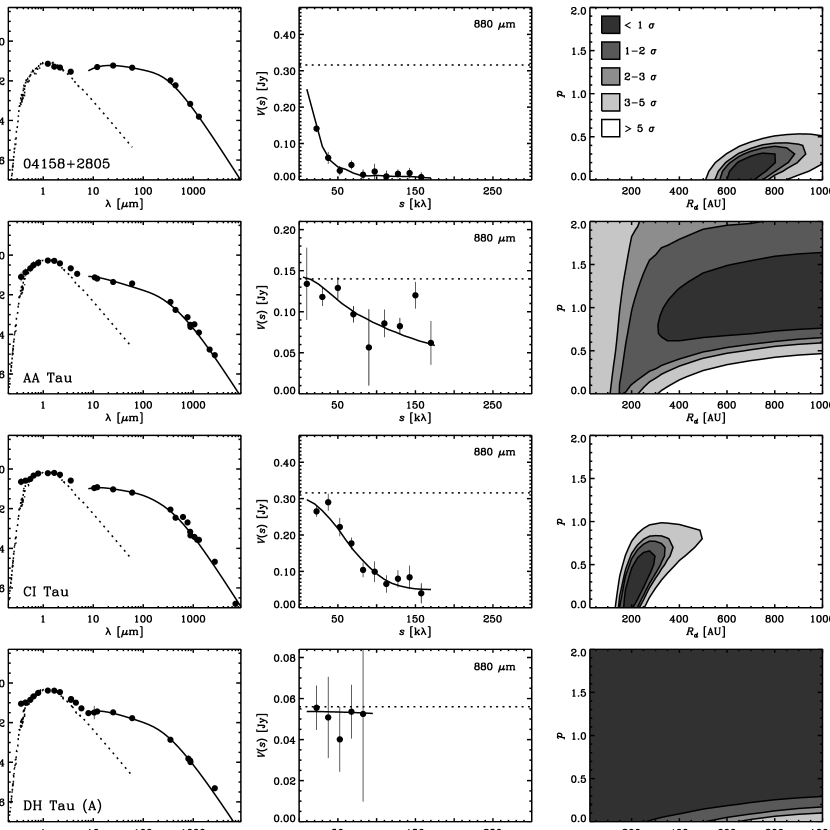
Figure 3: (left): De-reddened SEDs (defined so that $L_{\nu}=4\pi d^{2}\nu F_{\nu}$ in solar luminosity units). Dotted curves show Kurucz (1993) models of the stellar photosphere. (middle): Visibility profiles. The dotted line indicates the single-dish flux density scaled to the observing wavelength (labeled in the upper right corner for each disk) using a power-law fit to the submillimeter SED (see §4.2). (right): Maps of $\Delta\chi^{2}$ from the minimizations based on the flat disk model, projected into the {$R_{d}$, $p$}-plane. Contours and grayscale represent confidence intervals as indicated by the key in the top right panel. The best-fit models are overlaid on the SEDs and visibility profiles, generated with the parameters given in Table 4.

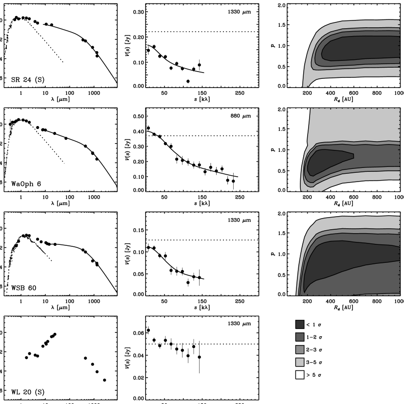
Figure 8: Same as Fig. 3.. Since no fit is performed for the Class I object WL 20 (S), we again show a key to the grayscale/contours in place of the $\Delta\chi^{2}$ map.

The remaining 5-parameter set {$T_{1}$, $q$, $\Sigma_{5}$, $p$, $R_{d}$} is constrained by the data using $\chi^{2}$-minimization. Figures 3$-$8 show the SED and visibility profile data with best-fit models overlaid, along with $\Delta\chi^{2}$ maps projected into {$R_{d}$, $p$}-space for the sample disks. The grayscale and contours in the $\Delta\chi^{2}$ maps represent confidence intervals ranging from $<1$ $\sigma$ to $>5$ $\sigma$ from dark to light, as indicated in the keys in Figures 3 and 8. The values of $p$ and $R_{d}$ were limited in the fitting to reasonable ranges; $p\in$ {0.0, 2.0} and $R_{d}\in$ {25, 1000}. The values of the other fitted parameters were determined by refining a search over a wide range to a smaller subset with a lower $\Delta\chi^{2}$ threshold (this is the same as the method devised by Lay et al., 1997). The resulting best-fit disk structure parameter values and their 1 $\sigma$ errors are compiled in Table 4, as well as total disk mass estimates ($M_{d}$, from a direct integration of the best-fit surface density profile), and values and references for the fixed parameter subset {$r_{0}$, $i$, PA}. The total reduced $\chi^{2}$ values for the sample range from 0.5 to $\sim$3, with a median value of $\sim$1.8. In many cases, much of the discrepancy between the model and the data can be attributed to absolute flux calibration uncertainties in the SED, particularly at submillimeter wavelengths where calibration accuracy is especially difficult.

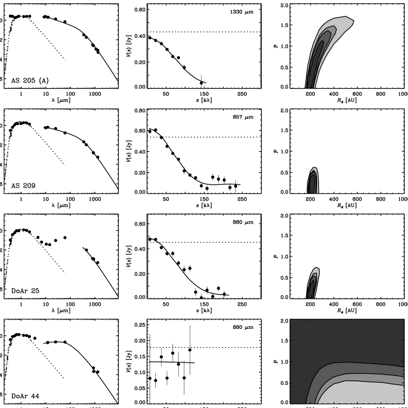
Figure 6: Same as Fig. 3.

The data for the Class I object WL 20 (S) was excluded from these fits because the SED has the clear steep rise in the infrared expected from extended envelope emission (see Fig. 8). Modifications to the minimization description above had to be made for 3 other disks in the sample. The DM Tau and GM Aur disks are known to have large central holes (i.e., large $r_{0}$; Calvet et al., 2005), which significantly affect their infrared SEDs and therefore the ability to infer their temperature distributions. In these cases, we have chosen only to model the submillimeter part of the SED ($\lambda\geq 350$ $\mu$m) and the continuum visibilities by fixing the temperature distribution. The adopted outer disk ($r\geq 30$ AU) temperature distributions are based on power-law approximations of the midplane temperature distributions computed by D’Alessio et al. (2005) from detailed models of irradiated viscous accretion disks. The D’Alessio et al. (2005) models were chosen to have central stars with roughly the same spectral types and ages ($\sim$1 Myr) as these disks, along with appropriate mass accretion rates (Ṁ $\approx 10^{-9}$ and $10^{-8}$ M_⊙ yr^-1 for DM Tau and GM Aur, respectively) and other standard disk properties ($\alpha=0.01$, grain size distribution index of 3.5, maximum grain size of 1 mm). The same procedure was adopted for DoAr 25 (assuming an age of 1 Myr and Ṁ $\approx 10^{-9}$ M_⊙ yr^-1), due to the peculiar morphology of the infrared SED (see Fig. 6). Although it may be more likely that the IRAS photometry for this source is contaminated by extended cloud emission, we can also not rule out a central hole similar to GM Aur, especially given the limit placed on the mass accretion rate, Ṁ $\lesssim 6\times 10^{-10}$ M_⊙ yr^-1 (Natta et al., 2006a).

3.4 Caveats and Parameter Relationships

Although the flat disk model is a computationally expedient approximation of a more detailed structure model, it contains a number of implicit assumptions which deserve to be highlighted. Of these, the most significant is the requirement that the spatial distributions of temperature and density follow power-law behaviors with the same index ($q$ and $p$, respectively) across the entire extent of the disk. Furthermore, the vertical structure of the disk is altogether ignored, despite the fact that flaring is expected based on hydrostatic equilibrium (Kenyon & Hartmann, 1987; Chiang & Goldreich, 1997, 1999). An over-simplified opacity function, particularly its presumed spatial uniformity in the disk, represents another critical assumption in the model. In general, each of the individual parameters in the flat disk model can have a significant impact on both the SED and visibility profile.

In a fit of the flat disk model to a dataset, the radial temperature profile (parameters {$T_{1}$, $q$}) is essentially fixed by the intensity and shape of the infrared SED. This is due to the fact that for the standard opacity prescription and any reasonable density values, the infrared emission generated in the inner disk is completely optically thick. In this case $(1-e^{-\tau_{\nu,r}\sec{i}})\approx 1$, and Equation 4 can be simplified so that

$$F_{\nu}\propto T_{1}^{2/q}\nu^{3-2/q}\cos{i},$$ (5)

where the normalization basically consists of physical constants (cf., Beckwith et al., 1990). In essence, the infrared SED is a sensitive diagnostic of the temperature profile, and not density. The parameters {$T_{1}$, $q$} can be determined through the SED alone, provided there are enough infrared datapoints. The important point is that the inner, optically thick part of the disk sets the temperature profile, which is assumed to extrapolate into the outer regions.

In contrast, the disk size and density profile (parameters {$\Sigma_{5}$, $p$, $R_{d}$}) wield significantly more influence over the emission at longer wavelengths. Assuming the disk is not too dense and the usual opacity law applies, most of the submillimeter emission should be optically thin (Beckwith et al., 1990). In this case $(1-e^{-\tau_{\nu,r}\sec{i}})\approx\tau_{\nu,r}\sec{i}=\kappa_{\nu}\Sigma_{r}\sec{i}$, and the flux density from Equation 4 becomes

$$F_{\nu}\propto\kappa_{\nu}\int_{r_{0}}^{R_{d}}B_{\nu}(T_{r})\Sigma_{r}\,r\,dr\propto\kappa_{\nu}\nu^{2}T_{1}\Sigma_{5}\int_{r_{0}}^{R_{d}}r^{1-p-q}\,dr\sim\frac{\kappa_{\nu}\nu^{2}T_{1}\Sigma_{5}}{(2-p-q)}R_{d}^{2-p-q},$$ (6)

where we have assumed that the the Rayleigh-Jeans limit applies and $R_{d}\gg r_{0}$. The integrand in the second proportionality gives the radial surface brightness, $I_{\nu}(r)$, and the visibility profile, $V_{\nu}(s)$, as its Fourier transform

$$I_{\nu}(r)\propto r^{1-p-q}\,\,\,\,\stackrel{{\scriptstyle\rm{FT}}}{{\longrightarrow}}\,\,\,\,V_{\nu}(s)\propto s^{p+q-3},$$ (7)

where $s=\sqrt{u^{2}+v^{2}}$ is the spatial frequency distance (cf., Looney et al., 2003). Equations 6 and 7 are simplified representations of a more complex situation. In reality some of the submillimeter emission is generated in the inner disk where optical depths are high, thereby complicating the parameter relationships (for details, see Beckwith et al., 1990). However, these relations are good first-order approximations and serve to illustrate a key component of the flat disk model: the outer, more optically thin part of the disk sets the density profile, which is then assumed to extrapolate into the inner regions.

To illustrate these dependencies with an example related to fitting real data, consider an adjustment that decreases the value of the power-law index of the surface density profile, $p$ (i.e., a redistribution of mass to larger radii). This would act to increase both the submillimeter flux densities and the surface brightness at larger radii, thus making the visibility profile drop off more rapidly at shorter spatial frequency distances (see Equations 6 and 7). Keeping in mind that the temperature profile is set in the infrared, compensating for the drop of $p$ in a fit would require a decrease in the surface density normalization ($\Sigma_{5}$) and/or outer radius ($R_{d}$). This interplay between parameters is a manifestation of the submillimeter emission in the outer disk being mostly optically thin. As would be expected, a sharp outer radius cutoff more strongly affects the observables for shallower density profiles (i.e., lower $p$), whereas the outer radius quickly becomes negligible (and thus poorly constrained) as the density profile steepens (see also Mundy et al., 1996).

The above discussion reiterates that the assumptions of single power-laws for the temperature and density across the entire disk are critical. Without them, we could not assume that the inner disk temperature profile is applicable in the outer disk or vice versa for the outer disk density profile. The other parameters that were fixed in the model have more complicated effects on the data. To start, the location of the inner radius really affects only the infrared SED, such that larger $r_{0}$ would decrease fluxes at those wavelengths. Generally this is not an issue, as the shorter infrared wavelengths are not used in the fits (however, see the Appendix regarding disks with large $r_{0}$). The effects of the opacity can be significant, and are discussed in their own right in the following sections.

The projected disk geometry, characterized by {$i$, PA} and fixed in the minimization algorithm used here, can significantly influence the other parameters in the flat disk model. Several of the disks in the sample have reliable geometry constraints from independent measurements (see the notes in Table 4), but in most cases we derive {$i$, PA} from elliptical Gaussian fits to the continuum visibilities. In such cases, a natural concern is that these Gaussian geometries do not represent the true disk geometries. To test the validity of using the Gaussian fits, we created synthetic continuum images using the flat disk formalism described above with a variety of parameter sets, inclinations, and orientations. These synthetic images were then “observed” in the same way as the data, for both the compact (C2) and extended (E) SMA configurations and with the appropriate thermal noise added to reproduce typical signal-to-noise levels. The geometries derived from elliptical Gaussian fits to the synthetic visibilities can then be compared to the known input geometries from the flat disk model. In general, the Gaussian inclinations yield fairly accurate results, but a few important points should be addressed. First, inclinations based on Gaussian fits are better approximations when surface brightness profiles are shallow (e.g., for lower values of $p$). Second, coverage in the Fourier plane is important: the Gaussian inclinations are more accurate with the combined C2+E array configuration (note that the C1 configuration is basically intermediate to the C2 and C2+E cases). And third, the Gaussian fits tend to slightly underestimate intermediate and high inclinations (by $\sim$10° at most), and overestimate low inclinations (by up to $\sim$15$-$20°).

To investigate the effects of fixing an erroneous value of the inclination in the fitting process, we also generated synthetic SEDs for the disk models described above. We then fit the synthetic SEDs and visibilities for a range of fixed inclination angles, and the best-fit parameter values were compared with the known input values. In general, fixing a value of $i$ that is lower than the true value leads to underestimates of other parameters, most importantly {$\Sigma_{5}$, $p$, $R_{d}$}. The magnitude of this effect depends on several conditions: the true inclination and how severely the assumed inclination underestimates it; the radial surface brightness distribution (i.e., $p$); the relative projections of the surface brightness distribution and the Fourier coverage of the interferometric observations; and the signal-to-noise ratio. As an example, consider a flat disk with a typical inclination of 60°. Given the underestimate of $i$ expected from a Gaussian fit, our simulations indicate that we could underestimate $p$ by up to $\sim$0.2$-$0.3 if the true value is $p\approx 1.5$. The underestimate of $p$ is insignificant if $p\lesssim 1$ (although the other parameters are changed). In the end, we are forced to adopt Gaussian inclinations as the best information available for many of the sources. In general, we are unlikely to overestimate the inclination in this way simply because nearly face-on disks should be relatively rare (assuming disk geometries are random). The sense of any effects on the parameters is then as described above, although the exact magnitude is generally unknown.

The analysis described above was also applied to better understand how fixing the disk orientation (PA) can affect the fitting results. Fortunately, the Gaussian fits effectively reproduce the true orientations in most cases within the errors (see Table 2). The exceptions are for low inclination angles (where the PA is basically meaningless anyway) or small radii. Again, any effects the PA could have on the visibility profile depend on the relative orientations of the projected disk emission and the sparsely-sampled Fourier coverage afforded by the observations. However, the agreement between the Gaussian fits and simulated data gives us confidence that fixing the disk orientations does not significantly affect the fitting results.

4 Results

4.1 Disk Structure

Keeping in mind the caveats discussed above, the combined fits of SEDs and visibilities provide constraints on basic structure parameters for the large number of circumstellar disks in this sample. Despite the simplicity of the adopted model and the remaining parameter uncertainties due to limited sensitivity and spatial resolution, we find the following: (a) the variation of temperature with radius is intermediate to the idealized cases of flat and flared disks; (b) small outer radii can be ruled out for most cases; and (c) the density apparently drops slowly with radius in the outer disk.

4.1.1 Disk Temperature Profiles

Figure 9 shows the distributions for the radial temperature profile parameters $T_{1}$ and $q$ for the sample. These histograms were created to crudely account for the uncertainties in the parameter measurements as follows. For each disk, we generate a Gaussian distribution normalized to have an area of 1 with a mean and standard deviation corresponding to the best-fit parameter value and error in Table 4. Parameters with asymmetric errors are allowed to have different standard deviations with a discontinuity at the mean (to ensure a total area of 1 for the distribution). All of the individual error distributions are then summed and binned (which effectively smooths away any discontinuities). In this way, the contribution of each disk to the histogram is appropriately weighted according to the uncertainty in the parameter measurement (e.g., Clayton & Nittler, 2004, see their Fig. 10). The median values for each parameter are shown with dotted vertical lines. The 1 AU temperatures in this sample have a clear, but fairly broad peak centered at $\sim$200 K.

The power-law indices (i.e., the radial slope of the temperature profile) also have a peak around the median value $q\approx 0.62$, with a few sources having substantially shallower temperature distributions (lower $q$). This peak in the distribution of the power-law index falls between the idealized values for the flat case, $q\approx 0.75$ (Adams et al., 1987), and the flared case, $q\approx 0.43$ (e.g., Chiang & Goldreich, 1997). This is probably the result of imposing a simple model upon a more complicated reality. For a typical disk, the temperature distribution is determined by the infrared SED from $\sim$8$-$60 $\mu$m, corresponding to emission produced roughly between $\sim$0.5$-$30 AU (give or take a factor of 2). In detailed physical models of disk structure, this corresponds to the region where vertical flaring begins to affect the temperature distribution; in essence, this is the transition region between the flat and flared scenarios (e.g., D’Alessio et al., 1998, 1999). It is therefore not so surprising that the typical single power-law index derived here lies between the two indices which better describe a more realistic disk structure.

This point is illustrated in Figure 10, which serves as a comparison of the typical temperature profiles measured here and those for more sophisticated models which self-consistently treat a variety of heating mechanisms in a more realistic two-dimensional disk structure (D’Alessio et al., 1998, 1999, 2005). The datapoints in this figure mark the median temperatures for the sample at various radii, determined based on the best-fit $T_{r}$ parameters listed in Table 4. The error bars show the first and third quartile temperatures to represent the range in the sample. The midplane radial temperature distribution for a detailed model of an irradiated accretion disk is also shown for comparison (cf., D’Alessio et al., 2005). The example model assumes a stellar mass of 0.5 M_⊙, effective temperature of 4000 K, and age of 1 Myr (all median values for the sample), and standard disk parameters (Ṁ = $10^{-8}$ M_⊙ yr^-1, $\alpha=0.01$, grain size distribution index of 3.5, and maximum grain size of 1 mm; see the descriptions in D’Alessio et al., 2005). In general, the simplified temperature distributions derived here turn out to be reasonable approximations of those determined with a more sophisticated treatment. However, the effects of the discrepancies between the simple approximations and the detailed models will be revisited below.

4.1.2 Disk Density Profiles

The distributions of the radial surface density profile parameters $\Sigma_{5}$ and $p$ are shown in Figure 11, created in the same way as for those in Figure 9. The distribution of $p$ should be treated with particular caution, as the errors on individual measurements are large. The disks with completely unconstrained $p$ values are not included in the distributions in Figure 11 or the analysis that follows. The distribution of $\Sigma_{5}$ has a broad peak around a median value of $\sim$14 g cm^-2. The distribution of $p$ indicates more disks in this sample have low values (i.e., less than $\sim$1) than high, with a median value of $p\approx 0.5$. The standard of reference often used in discussing the density distribution in circumstellar disks is the minimum mass solar nebula (MMSN), the progenitor circumstellar disk around the Sun. The MMSN density distribution is constructed by augmenting the masses of the planets in the solar system until cosmic abundance values are obtained, and then smearing the mass out into annuli centered on each planet’s semimajor axis (Weidenschilling, 1977). A simple power-law fit to the MMSN surface density distribution indicates $\Sigma_{5}\approx 150$ g cm^-2 and $p\approx 1.5$ (Hayashi et al., 1985), both of which are marked in Figure 11. As a second reference case, a steady-state viscous accretion disk has $p\approx 1$, while the normalization depends on a variety of other parameters (e.g., Hartmann et al., 1998).

The best-fit values of $p$ for this sample, while not very strongly constrained, often indicate that the density drops off more slowly in the outer disk than is expected from either the MMSN or the standard viscous accretion disk models. This is illustrated in Figure 12, where again a comparison can be made between the sample median density distribution and a more sophisticated disk structure model. As with Figure 10, we plot sample median surface densities at some representative radii (determined from the best-values of {$\Sigma_{5}$, $p$} in Table 4), with error bars marking the first and third quartiles as an indication of the range in the sample. Overlaid on the plot as a solid curve is the density distribution for the same irradiated accretion disk model described above for Figure 10 (cf., D’Alessio et al., 2005). The MMSN density distribution is also plotted as a dashed line. Observational measurements of the value of $p$ in circumstellar disks are critical to developing a better understanding of disk evolution and the planet formation process. Therefore, an examination of possible causes for the apparent disagreement between the typical values measured here ($p\lesssim$ 1 in most cases) and those expected from theory ($p\gtrsim 1$) is necessary.

In §3.4, we already highlighted a possible cause of artificially low values of $p$ in this sample; namely, underestimates of the true disk inclination angles. To examine this issue in more detail, we look at the cases where independent inclination estimates are available (see col. 11 in Table 4). For these disks, the median best-fit value of $p$ remains the same as for the full sample, $\sim$0.5. Therefore, for at least some of the disks in this sample, the low measured values of $p$ do not arise from erroneous inclination values. Without individual constraints on $i$ for the remaining sample disks, we are forced to rely on the Gaussian fits. As discussed in §3.4, any induced decrease in $p$ is typically expected to be small ($\sim 0.2-0.3$ if $p>1$).

Another potential issue with the surface density constraints could arise due to the simplified treatment of the disk temperature distribution. As mentioned above, detailed disk models indicate that the temperatures in the outer disk have a relatively shallow dependence on radius (due to vertical flaring) compared to the inner disk, where the temperature distribution is actually constrained by the data (Chiang & Goldreich, 1997; D’Alessio et al., 1998, 1999). Because of the single power-law assumption for $T_{r}$ made here, the derived power-law indices ($q$) are usually at intermediate values to the flat and flaring regimes in a more realistic disk. This implies that our temperature distributions could be too steep in the outer regions; the values of $q$ may be too high. If we were to adopt a lower value of $q$ more consistent with the detailed models, Equation 7 indicates that the value of $p$ should be increased in order to maintain the shape of the visibility profile. Therefore, the simplified temperature description used here could lead to underestimates of the surface density power-law index, $p$. In essence, since the quantity $p+q$ is well-constrained by the visibility profile, $\Delta p\approx-\Delta q$. This should only lead to modest increases on the order of $\Delta p\approx 0.2-0.3$, corresponding to the expected difference between the typical measured $q$ values and the flared disk $q$ values.

Other simplified assumptions in the model are not expected to significantly affect our determination of the power-law index of the density distribution. One such example is the assumed sharp outer disk boundary, compared to the exponentially decreasing density profile expected from the similarity solutions for viscous accretion disks (Lynden-Bell & Pringle, 1974; Hartmann et al., 1998). Using the solutions described by Hartmann et al. (1998), we generated synthetic SEDs and visibilities with reasonable errors and modeled them with the procedure described in §3. As one might expect, these simulations generally reproduce the correct value of $p$, or even slightly higher values due to the steep exponential drop-off in the outer disk. Therefore, the assumption of a sharp outer boundary does not factor into the low $p$ values inferred for much of our sample. In the end, there are two compelling reasons that may explain the shallow outer disk density distributions: over-simplified temperature distributions and possible inclination underestimates. The correction for the former is expected to be an additive increase $\Delta p\approx 0.2-0.3$. The magnitude of the adjustment to $p$ for the latter is more difficult to predict. Assuming that most of the disks in this sample have an intermediate inclination, we estimate that the correction is typically $\Delta p\approx 0.1$. Given the rather poor constraints on $p$ in general and these implied corrections, we suggest that the typical disk in this sample has $p\approx 0.7-1.0$.

4.1.3 Disk Sizes and Masses

In addition to the density structure, the spatially resolved SMA measurements provide valuable new constraints on circumstellar disk sizes. The top panel of Figure 13 shows the distribution of the outer disk radii for this sample, constructed in the same way described above for the temperature and density profile parameters. The distribution has a peak near the median radius of $\sim$200 AU, with a roughly Gaussian shape and extended large radius wing. Most of the disks are at least partially resolved, with radii larger than $\sim$100 AU. The values of $R_{d}$ measured here technically represent some characteristic radius beyond which the temperature/density conditions in the disk do not produce substantial submillimeter emission compared to the noise levels in the data. True disk sizes could be larger, but would have to be measured with more optically thick tracers like molecular line emission (e.g., Simon et al., 2000) or optical silhouettes (e.g., McCaughrean & O’Dell, 1996). Finally, as a caution it should be emphasized that elliptical Gaussian fits to interferometer data tend to underestimate disk sizes (compare the FWHM sizes in Table 2 with the $R_{d}$ values in Table 4). The problem is really one of contrast, so that the level of discrepancy increases dramatically for more centrally-concentrated surface brightness distributions (e.g., for higher values of $p$).

Armed with constraints on both the density distribution and size of the disk, the total mass is computed by simply integrating the surface density over the disk area. The distribution of disk masses for the sample is shown in the bottom panel of Figure 13. A broad peak is seen around the median mass of 0.06 M_⊙. It is important to emphasize again that the sample selection criteria explicitly introduce a bias toward more massive disks, and so this distribution in particular is not representative of the typical T Tauri disk (Andrews & Williams, 2005). Despite the rather large uncertainties in the density distribution and radius parameters, the inferred disk masses are constrained within a factor of 2. This is due to the low optical depths where the density and radius parameters are measured. Larger uncertainties in the disk masses are due to our limited knowledge of the opacity and the density structure in the inner, optically thick regions of these disks (both unaccounted for in Table 4 and Figure 13; see §5).

No statistically significant correlations between the best-fit disk structure parameters and properties of the central stars (e.g., $T_{*}$, $M_{*}$, age) or other disk diagnostics (e.g., Ṁ) were found for this sample. Only a marginal trend of increasing 1 AU temperatures for earlier spectral types is noteworthy. Neither are there any significant differences between disk structure properties among single and multiple star systems, or the two different star-forming regions incorporated into the sample. This is perhaps not so surprising, considering the limited ranges of star/disk properties in a sample of this size and the remaining uncertainties on the structure parameters.

4.2 Opacity

Perhaps the greatest uncertainties in studies of circumstellar disks are related to the growth of grains into larger solids and how this process subsequently shapes the structure, dynamics, and evolution of disk material (see Beckwith et al., 2000; Dominik et al., 2006). In the high density environment of a circumstellar disk, dust grains are expected to grow via collisional agglomeration and gravitationally settle toward the midplane of the disk. Observational evidence for the combined effects of grain growth and sedimentation have been accumulating from a variety of techniques (see the review by Natta et al., 2006b). At submillimeter wavelengths, the growth of solids in the disk is manifested as a change in the opacity spectrum, and therefore the shape of the continuum SED. Increased grain growth leads to grayer opacities and more efficient submillimeter emission (i.e., a shallower SED slope; e.g., Beckwith & Sargent, 1991; Calvet et al., 2002; Natta et al., 2004). The key affected parameter is the power-law index of the opacity spectrum, $\beta$, which is expected to decrease as a result of the grain growth process (Miyake & Nakagawa, 1993; Pollack et al., 1994; Krügel & Siebenmorgen, 1994; Henning et al., 1995; Henning & Stognienko, 1996; D’Alessio et al., 2001, 2006; Draine, 2006).

For an optically thin disk in the Rayleigh-Jeans limit, Equation 6 shows that the submillimeter SED has a power-law behavior with frequency, $F_{\nu}\propto\kappa_{\nu}\nu^{2}\propto\nu^{2+\beta}$. In this case, one could simply fit the observed SED with a general form $F_{\nu}\propto\nu^{n}$ and determine the opacity index, $\beta=n-2$, directly. However, the submillimeter emission may not be completely optically thin. Some optically thick emission, for which $F_{\nu}\propto\nu^{2}$, would serve to decrease the measured quantity $n$ and result in misleadingly low values of $\beta$. Therefore, the ratio of optically thick to thin emission, $\Delta$, needs to be explicitly calculated to translate the measured submillimeter SED power-law index, $n$, into the opacity index, $\beta$, via the simple approximation $\beta\approx(n-2)(1+\Delta)$ (cf., Beckwith et al., 1990; Beckwith & Sargent, 1991). The ratio $\Delta$ depends on wavelength and the disk structure (particularly {$q$, $\Sigma_{5}$, $p$, $R_{d}$, $i$}). Multiwavelength submillimeter photometry from single-dish telescopes and reasonable assumptions for $\Delta$ indicate that $\beta\approx 1$ for a large number of circumstellar disks (Weintraub et al., 1989; Beckwith & Sargent, 1991; Mannings & Emerson, 1994; Andrews & Williams, 2005). This is significantly lower than the value for the interstellar medium, where $\beta_{\rm{ISM}}\approx 1.7$ (Hildebrand, 1983; Weingartner & Draine, 2001), indicating an evolution in the opacity spectrum that could be due to the growth of grains. High-resolution interferometric work has allowed measurements of $\Delta$ and therefore less ambiguous constraints on $\beta$, adding further evidence for the presence of large grains in a variety of disks (e.g., Testi et al., 2001, 2003; Natta et al., 2004; Wilner et al., 2005; Rodmann et al., 2006).

Following the method described above, Table 5 lists the measured values of $n$, $\Delta$, and $\beta$ for the sample disks. The SED power-law indices, $n$, were determined using only wavelengths longer than 850 $\mu$m (or 1 mm whenever possible) to ensure that the Rayleigh-Jeans criterion holds. Based on the temperatures at the outer disk edges, any corrections for violating this criterion would lead to only modest increases in $n$ (generally within the 1 $\sigma$ error bars). For each disk, the ratio of optically thick to thin emission, $\Delta$, at the shortest wavelength used in determining $n$ was computed for each parameter combination corresponding to the regions in Figures 3$-$8 within the 1 $\sigma$ confidence interval. Listed in Table 5 are the maximum $\Delta$ values inferred from these regions (usually those for the highest $p$ and smallest $R_{d}$). Figure 14 shows the distribution of $\beta$ values calculated for this sample, created in the same way as other distributions presented here to account for the large error bars. The median value is $\beta\approx 0.7$, considerably lower than for the interstellar medium, and consistent with the typical estimates for circumstellar disks.

However, this indirect method of deriving $\beta$ from the submillimeter SED and disk structure models contains some circular logic. For a given disk, the value of $\Delta$ depends on the best-fit structure parameters, which were derived based on an assumed opacity spectrum. As an experiment to determine the influence of $\beta$ on the disk structure parameters, we fitted the data for a typical disk (WaOph 6) with a range of $\beta$ values. The surface density normalization, $\Sigma_{5}$, proves to be the most dramatically affected parameter due to changes in $\beta$. For the mostly optically thin submillimeter emission, the optical depth ($\tau_{\nu,r}$) is well-determined by the flux, and therefore $\Sigma_{r}\propto\kappa_{\nu}^{-1}$. So, for a fixed $\kappa_{0}$ an increase in $\beta$ leads to a drop in $\kappa_{\nu}$, and subsequently an increase in $\Sigma_{5}$ to compensate for the observed emission. As long as the emission at infrared wavelengths remains optically thick, the temperature distribution parameters are not significantly affected. For larger variations of $\beta$ (e.g., $\pm 1$), there can also be substantial changes in {$p$, $R_{d}$}, such that a larger $\beta$ leads to a larger radius and a smaller value of $p$. As an aside in the context of the discussion in §4.1.2, note how this implies that our assumption of a $\beta$ value lower than in the interstellar medium is also not responsible for artificially decreasing the measured $p$ values.

The above simulations imply that the optically thick area of the disk does not change significantly for different input $\beta$ values, and therefore the value of $\Delta$ remains roughly the same. Given this tendency for self-correction, the method of determining $\beta$ by adjusting the measured SED slope, $n$, to accomodate an optically thick contribution is a reasonable approximation. However, the smaller changes in {$R_{d}$, $p$} noted for different assumed $\beta$ values do have the capability to affect $\Delta$. Because of the interplay between these parameters, a better way to determine $\beta$ is by allowing it to be a free parameter in the fits, a task usually accomplished by fixing $p$ instead. Given the data in hand, the addition of $\beta$ as another free parameter in the fits described here unfortunately does not provide any statistically meaningful constraints (without fixing other currently free parameters). However, this could be accomplished either with multiwavelength interferometric data (e.g., Lay et al., 1997) or data with very high quality and resolution (see Hamidouche et al., 2006).

As Table 5 indicates, we can not provide reliable estimates of $\beta$ for a number of disks in this sample for two primary reasons. First are the cases where the submillimeter emission is either not spatially resolved (e.g., FT Tau) or highly optically thick due to the disk inclination (e.g., RY Tau), and therefore $\Delta$ (and thus $\beta$) could be arbitrarily high. For these disks we quote only lower limits on $\beta$ based on the assumption that $\Delta\geq 0$. And second are the cases where the observed power-law index of the submillimeter SED, $n$, is less than 2. The submillimeter SED can have $n<2$ for a variety of reasons, including low disk temperatures (i.e., the Rayleigh-Jeans criterion fails), extensive dust sedimentation (D’Alessio et al., 2006), simple statistical errors, or contamination from extended and/or non-disk emission (e.g., non-thermal emission from a stellar wind). Unfortunately, the latter possibility of extended emission contamination, perhaps from residual envelopes surrounding the star/disk systems, seems to be especially likely for the more embedded sources in the Ophiuchus star-forming region. A more reliable measurement of $n$ for these sources will require interferometric observations at a second wavelength to ensure that only compact disk emission is included in the SED fits.

5 Discussion

Including those presented here, roughly 40 circumstellar disks around T Tauri stars have been observed with (sub)millimeter interferometers at a variety of wavelengths and resolutions. Nearly half of the 24 disks in this survey have been previously observed (AA Tau, CI Tau, DL Tau, DM Tau, DN Tau, DR Tau, FT Tau, GM Aur, RY Tau, AS 209, and WL 20; Koerner et al., 1993; Koerner & Sargent, 1995; Dutrey et al., 1996, 1998; Guilloteau & Dutrey, 1998; Looney et al., 2000; Simon et al., 2000; Barsony et al., 2002; Kitamura et al., 2002; Dartois et al., 2003; Rodmann et al., 2006). An unbiased comparison of disk structure constraints in the literature would be a nearly impossible task, due to the wide diversity of data and models adopted for different disks. Nevertheless, it is worthwhile to summarize what has been observationally inferred about disk structure from the perspective of high resolution submillimeter measurements.

There are relatively few constraints on the density distribution in these disks. This is partly due to limited sensitivity and resolution, but also due to a common preference to constrain other parameters instead (e.g., {$i$, $\beta$}). In that case, $p$ is usually fixed in the modeling to ensure a reasonable number of degrees of freedom and useful measurements of the interesting parameters. When not fixed, a wide range of $p$ values have been noted. One method to determine disk structure utilizes spectral images of CO rotational transitions and the submillimeter portion of the SED with a model similar to that described here, but including a flared vertical structure (Guilloteau & Dutrey, 1998). In most cases this technique restricts the value of $p$, but the results provide good fits to the data for values near 1.5 (Dutrey et al., 1998; Guilloteau & Dutrey, 1998; Dartois et al., 2003; Dutrey et al., 2003). Other methods have more in common with those used here, based on both high resolution submillimeter continuum data and the SED. These lead to a considerable range of $p$ values, from 0$-$1.5, depending on the individual disk and which data are used in the modeling (Mundy et al., 1996; Lay et al., 1997; Akeson et al., 1998, 2002; Kitamura et al., 2002; Duchêne et al., 2003). The only other large collection of $p$ measurements to date is from the 2 mm survey of Kitamura et al. (2002); their work shows a median $p\approx 0.6$, similar to the value presented here. If we take at face value all of the available measurements of $p$ determined with the flat disk model, the distribution is similar to that presented in Figure 11, again with a median value of $\sim$0.5. Upon consideration of the potential systematic underestimates of $p$ for these simple models (see §4.1.2), the typical disk probably has a value closer to $p\approx 0.7-1.0$.

In terms of the outer disk radius, the silhouette disks and proplyds in the Orion nebula provide an interesting comparison to the SMA sample. Vicente & Alves (2005) compute disk sizes for 149 such objects in a homogeneous way. Their resulting distribution of $R_{d}$ has a similar shape to that seen in the top panel of Figure 13, but the peak is substantially shifted to smaller radii. The median proplyd disk radius is $\sim$70 AU, while the subsample of silhouette disks has a median radius of $\sim$135 AU. A Kolmogoroff-Smirnov test confirms that the Orion disks are significantly smaller than the disks in Taurus and Ophiuchus, where the median radius is $\sim$200 AU. This difference is not likely to be an artifact of how the radii are measured. The characteristic radii inferred from optical observations are expected to be systematically larger than those at submillimeter wavelengths because the much higher optical depths at shorter wavelengths allow material to be traced out to lower densities (and thus larger radii). The reason for the different disk sizes in Orion is most likely related to the local environment, perhaps due to dynamical interactions in a higher stellar density cluster and/or the intense external photoevaporation from nearby massive stars (e.g., Johnstone et al., 1998). The disks in the Taurus and Ophiuchus star-forming regions do not have to contend with such extreme environments, and therefore have larger sizes than those in Orion despite their similar ages.

5.1 Accretion Disks

The values of $p$ inferred above are similar to the expectations for steady-state viscous accretion disks (Hartmann et al., 1998; D’Alessio et al., 1998, 1999; Calvet et al., 2002). This is also in good agreement with the $p\approx 1$ inferred for the carefully studied TW Hya disk in the context of those models (Wilner et al., 2000). In the standard similarity solutions for the structure of an accretion disk, the surface density power-law index ($p$) corresponds to the power-law index ($\gamma$) for the radial distribution of the viscosity (e.g., Lynden-Bell & Pringle, 1974; Hartmann et al., 1998). An independent constraint on $\gamma$ can be obtained via measurements of the decay of mass accretion rates with time, in essence of $\eta$ in the scaling relation Ṁ $\propto t^{-\eta}$ (Hartmann et al., 1998, see their Eqn. 28). Using the accretion rates of young stars in the Taurus and Chameleon star formation regions, Hartmann et al. (1998) inferred that $\eta\approx 1.5-2.8$, or equivalently $\gamma\approx 1.0-1.7$, with a preference for the lower value based on an assessment of the more likely systematic errors. While these measurements of {$p$, $\eta$} have fairly large uncertainties, both are consistent with the viscosity being distributed with a roughly linear dependence on radius in the outer parts of circumstellar disks.

In such a case, the $\alpha$ parameter for the viscosity (Shakura & Sunyaev, 1973; Pringle, 1981) can be considered constant over the timescales of interest for these disks (Hartmann et al., 1998). The $\alpha$ parameter essentially characterizes the level of turbulent viscosity in the disk, and therefore the rate at which the disk structure evolves; the sense is that lower values of $\alpha$ (i.e., less turbulent viscosity) correspond to slower evolution. Angular momentum conservation leads to the expansion of accretion disks to larger radii, where the rate of expansion basically depends upon $\alpha$, the mass of the central object ($M_{*}$), and the initial disk conditions. Assuming these initial conditions are roughly similar for T Tauri disks, the observed time variation of disk properties can be useful tools to estimate the value of $\alpha$. Disk sizes are of particular interest in this case.

However, the meaning of the sharp boundary $R_{d}$ measured in this paper is unclear in the context of the accretion disk models, where instead the density distribution is allowed to drop off exponentially. The values measured here really correspond to a sensitivity limit to the surface brightness profile of the continuum emission. To empirically relate our values of $R_{d}$ with some characteristic radius in the accretion disk formalism described by Hartmann et al. (1998), we have used the same fitting scheme described in §3 to model simulated accretion disk SEDs and visibilities at various evolutionary stages. The results for a fiducial model (see below) generally indicate that $R_{d}$ corresponds to an accretion disk radius that encircles a large fraction $f$ of the total disk mass (cf., Hartmann et al., 1998, their Eqn. 34). For $\alpha=0.01$, the value of $f$ decreases smoothly from nearly 1 at $10^{5}$ yr to $\sim$0.5 at $10^{7}$ yr. When $\alpha=0.001$, $f\approx 1$ before $10^{6}$ yr, where it begins to drop to $\sim$0.7 by 10⁷ yr.

Figure 15 shows plots of 850 $\mu$m flux densities, mass accretion rates, disk radii, and Gaussian FWHM sizes as a function of stellar age for this sample. Values of Ṁ and ages were gathered from the literature, and are listed for individual disks in Table 3. Overlaid on these plots are the expected evolutionary behaviors of these disk properties based on the $\gamma=1$ similarity solutions for viscous accretion disks of Hartmann et al. (1998, cf. their §4.3.1) for a fiducial parameter set. Here we have fixed the initial disk mass to 0.1 M_⊙, the stellar mass to 0.5 M_⊙, the initial scaling radius to $R_{1}=10$ AU, $d=150$ pc (the average between the two regions used here) and have let $T_{r}\propto r^{-0.5}$ with a normalization of 200 K at 1 AU (the median value found here). These models were computed for two values of $\alpha$; 0.01 (solid curves) and 0.001 (dashed curves). The 850 $\mu$m flux densities for these accretion disk models were calculated using our Equation 4, with the surface density profile described by Hartmann et al. (1998, their Eqn. 33) and enforcing a minimum disk temperature of 7 K. The evolutionary behavior of the mass accretion rates shown in Figure 15 were computed at $r=0$, following Hartmann et al. (1998, their Eqn. 35).

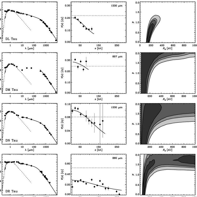
Figure 4: Same as Fig. 3.

The variation of the disk radius with time, shown in the lower left panel of Figure 15, corresponds to the accretion disk model prediction $R_{d}\propto R_{1}\mathcal{T}$, where $R_{1}$ is a scaling radius (encircling $\sim$60% of the disk mass at $t=0$), $\mathcal{T}$ is a scaling time related to the number of viscous timescales that have passed, and the constant of proportionality is determined by the empirically measured $f$ value described above. The time variation of the Gaussian FWHM size for these accretion disk models were determined by “observing” synthetic images with the SMA C1 array configuration and fitting directly to the visibilities. The datapoints plotted in this panel are FWHM values determined only from compact SMA configurations for ease of comparison (there is no significant difference between C1 and C2 for this purpose). Different model curves and datapoints are shown for 880 and 1330 $\mu$m. Note that the evolutionary pattern of the model FWHM sizes here and that shown by Hartmann et al. (1998, their Fig. 4) are different. This is due to our use of a fit to the visibilities, while they chose to convolve the image with a synthesized beam-sized Gaussian. If their technique is adopted, we do reproduce the FWHM behavior shown in that paper.

For a more direct comparison of the observable data with the accretion disk model predictions, Figure 16 shows a sample median SED and median visibility profiles at 880 and 1330 $\mu$m. Error bars represent the first and third quartiles at each wavelength or spatial frequency distance. The visibility profiles are normalized at a spatial frequency distance of $\sim$20 k$\lambda$, and no correction is attempted to account for the slightly different distances to the two star-forming regions where the sample disks are located. Overlaid on the median datapoints are the accretion disk models described above. An examination of the evolutionary behaviors of submillimeter emission, mass accretion rates, and disk sizes in Figure 15 and the corresponding typical SED and spatial distribution of emission in Figure 16 indicate that the $\gamma=1$ similarity solution for a fiducial viscous accretion disk model with $\alpha=0.01$ generally describes a wide range of observed disk properties remarkably well. The fiducial model with a lower value of $\alpha$ (i.e., less turbulent viscosity) tends to over-predict submillimeter fluxes and accretion rates and under-predict disk sizes. While an increase of $R_{1}$ to $\sim$100 AU in this case would help in explaining the observed disk sizes and spatial emission distribution, it would also result in very little evolution in both the submillimeter fluxes and accretion rates, contrary to the observed trends. The reader is referred to the work of Hartmann et al. (1998) regarding the effects of variations in other parameters. We conclude that viscous accretion disks with $\alpha=0.01$ provide the best general description of the observational properties of the disks in this sample.

5.2 Planet Formation

In terms of utilizing the density structure of circumstellar disks to better understand the planet formation process, we can compare with the MMSN and a similar minimum mass “extrasolar” nebula (MMEN; Kuchner, 2004) as references. Unfortunately, these are not necessarily valuable comparisons. First, the interferometer data and MMSN/MMEN are providing information about different regions in disks; a direct analogy between the two is still limited by the spatial resolution of the data. And second, while the circumstellar disk observations provide a measurement of $\Sigma_{r}$ at one instant in an evolution sequence, the MMSN and MMEN refer to the density structure integrated over the entire evolutionary history of the solar and extrasolar disks. In the later evolutionary stages when planetary embryos have formed and can dynamically influence the disk structure, it would not be so surprising if the density distribution varied significantly from the $p\approx 1$ expected for a steady-state accretion disk.

In that sense, it is not too much of a concern that the inferred $p$ values for disks generally appear to be different than the $p\approx 1.5-2$ based on a fit to augmented planetary masses (Weidenschilling, 1977; Hayashi et al., 1985; Kuchner, 2004). Moreover, it has been suggested that a double power-law behavior of the MMSN density distribution is more reasonable. For example, Lissauer (1987) points out another scenario where $p\approx 0.5$ for radii less than $\sim$10 AU and $p\approx 1$ for larger radii. This prescription is in rather good agreement with detailed accretion disk models (D’Alessio et al., 1998, 1999). Raymond et al. (2005) point out that, as long as there is sufficient material available, the ability to form planets does not strongly depend on $p$. Therefore, the real issue of comparison between the observations of circumstellar disks and the requirements of planet formation models lies more with the normalization, and not the shape, of the density distribution. The important constraint is on how much mass is packed into the area where planets are thought to form.

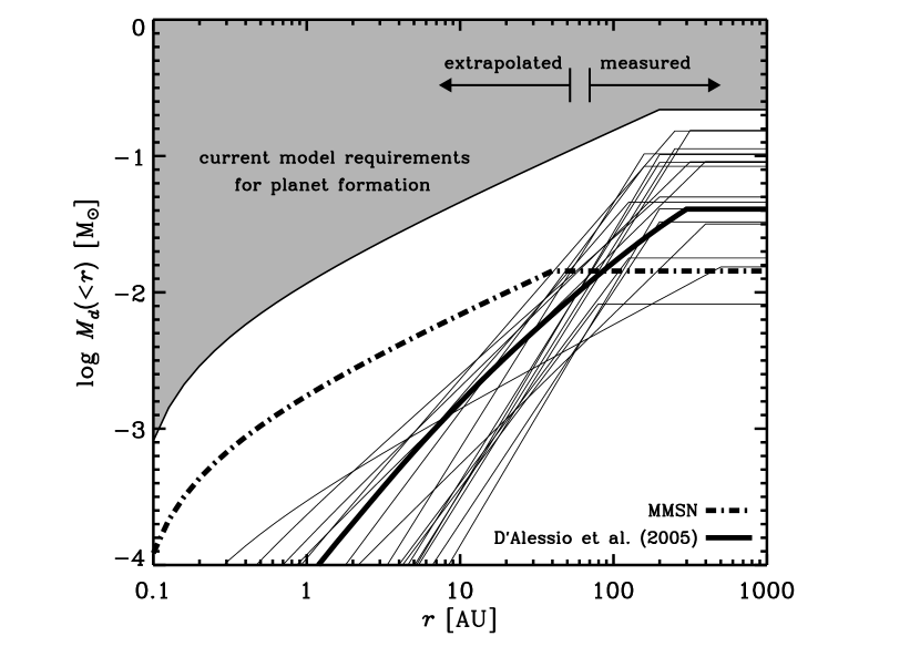
Figure 17: Cumulative disk masses (i.e., the mass internal to $r$) as a function of radius for the sample (thin solid curves), determined with the best-fit surface density parameters listed in Table 4. The gray area roughly marks the density requirements for current planet formation models. The lower boundary of this region corresponds to $\Sigma_{5}=10^{3}$ g cm^-2 and $p=1.5$ for a disk truncated at 200 AU. The heavy dashed curve marks the Hayashi et al. (1985) MMSN values with an outer radius of 50 AU. The integrated surface density profile for the irradiated viscous accretion disk model calculated by D’Alessio et al. (2005) and described in the text (see Fig. 12) is also shown as a heavy solid curve. The current observational estimates of densities in the disk fall short of the values required by planet formation models, perhaps in part due to an overestimate of opacities.

Regardless of whether planets are created by core accretion and gas capture (e.g., Pollack et al., 1996; Inaba et al., 2003), gravitational instability (e.g., Boss, 1998, 2005), or a hybrid scenario (e.g., Durisen et al., 2005), all of these models require total masses in the inner disk at least one order of magnitude higher than the values inferred here from the constraints on $\Sigma_{r}$. This is illustrated schematically in Figure 17, where we have used the best-fit values of {$\Sigma_{5}$, $p$} in Table 4 to plot cumulative disk masses (the total mass internal to radius $r$) as a function of radius for the disks in this sample. The shaded region in this figure corresponds to the surface density parameters required to provide at least $\sim$0.1 M_⊙ of material within a radius of 20 AU, the typical prerequisite values for current planet formation models. Taking the disk structure constraints at face value would suggest that these disks will not be capable of forming planets on reasonable timescales. However, this is not necessarily the case. As we have emphasized above, the density distribution is currently only measured in the outer disk (beyond $\sim$60 AU at best) and the densities in the inner disk are extrapolated from these measurements assuming a very simple structure model. Without higher resolution data capable of tracing the inner disk material, we simply do not have a direct constraint on densities in the regions of interest for planet formation.

There is one particularly notable way to reconcile the observationally inferred densities and those required by planet formation models: adjustments to the disk opacity. The analysis in §4.2 and a number of other studies indicates that dust grains in the outer disk have grown to millimeter-scale sizes. The presence of a substantial population of centimeter-scale solids has even been inferred for the outer regions of the TW Hya disk (Wilner et al., 2005). Considering the expected strong radial dependence of collision timescales in the disk, and thus the growth timescales modulo some coagulation probability, a significant population of even larger solids could exist near the midplane in the inner parts of these disks. Obviously, without a proper accounting of larger solids and their distribution with radius in the disk, the opacity formalism adopted in our models is unfortunately primitive and insufficient. Because the growth process would serve to decrease the opacity, reproducing the observed levels of disk emission would require a substantial increase in the densities (particularly for the inner disk). Indeed, the models by D’Alessio et al. (2001, their Fig. 3) indicate significantly decreased opacities when the maximum grain size is larger or smaller than a few millimeters. Of equal importance is the implicitly assumed mass ratio of gas to dust in the disk midplane. Here we assume the dust phase contributes only $\sim$1% of the mass, as in the interstellar medium. However, given the preferential sedimentation of larger solids to the midplane, it would not be surprising if the solid mass fraction in the regions responsible for the continuum emission was substantially higher. Larger solid mass fractions would also imply proportionately smaller opacities, and thus higher densities (see also Youdin & Shu, 2002).

In light of all this, it is likely that our extrapolated estimates of densities in the inner disk are significantly underestimated, at least in part due to a vastly over-simplified prescription for the opacity. If the average opacity is roughly an order of magnitude lower than we assume, the densities in the typical disk should be sufficient to form planetary systems (the issue then becomes deciding which formation mechanism is more likely). Unfortunately, diagnosing the effects of grain growth on the observable data for any individual disk is a daunting task. One has to be concerned not only with the complicated growth and sedimentation processes (D’Alessio et al., 2001, 2006; Dullemond & Dominik, 2004, 2005), but also the structural, mineralogical, and dynamical properties of the aggregate solids (e.g., Wright, 1987; Henning et al., 1995; Takeuchi & Lin, 2005). So, while we might not be able to determine with great certainty the magnitude of the effects of these processes on the inferred disk densities, the sense that they are underestimated is fairly certain.

5.3 Future Work

The prospects for significant improvements on basic disk structure measurements are excellent. The current suite of interferometers (SMA, PdBI, NMA, VLA) operate in all of the major atmospheric windows beyond $\sim$450 $\mu$m with a typical spatial resolution of $\sim$1″ and the potential to improve up to a factor of $\sim$3 higher. The CARMA interferometer will provide a substantial increase in sensitivity and resolution, where its kilometer-scale baseline lengths will allow direct probes of the density into the inner regions ($r\lesssim 20$ AU) of nearby disks. We have briefly explored the potential advances in constraining the power-law index of the density distribution ($p$) via modeling simulated flat disk data for various observational facilities. For a typical disk with $p=1$ and $R_{d}=200$ AU, the standard setups for current interferometers can potentially measure $p$ to within roughly $\pm$0.3$-$0.4 (e.g., see the WaOph 6 disk in Figure 8 with the SMA C2+E configuration). The accuracy of the constraint on $p$ basically increases linearly with the spatial resolution, indicating that kilometer-scale CARMA baselines should be capable of measuring $p$ to within $\pm$0.1. The added benefit of improved spatial resolution is the sensitivity to the density distribution on ever smaller spatial scales in the disk, probing into the region where giant planets are expected to form. The real key to realizing this potential lies primarily with the ability to make phase corrections on the longest baseline separations (e.g., using water-vapor radiometry).

The promise of submillimeter data with higher sensitivity and resolution will also allow some of the restrictions in the modeling described here to be relaxed. The obvious goal will be to switch some of the fixed parameters into free ones (for example, fitting for the disk geometry directly from the 2-D distribution of visibilities). Of particular interest in this case is letting the power-law index of the opacity spectrum ($\beta$) be a free parameter, rather than relying on the approximate correction to the observed SED slope discussed in §4.2. Ideally, this would be done in a direct way by adopting a model adjustment to simultaneously fit interferometric data at multiple wavelengths (e.g., Lay et al., 1997). Almost all interferometers have a simultaneous dual-wavelength capability well-suited for this kind of analysis.

6 Summary

We have used the SMA interferometer to conduct a high spatial resolution submillimeter continuum survey of 24 circumstellar disks in the Taurus-Auriga and Ophiuchus-Scorpius star formation regions. By simultaneously fitting the broadband SEDs and submillimeter continuum visibilities to a simple disk model, we have placed constraints on the basic structural properties of these disks. We find:

1. The radial distributions of temperature and density in these disks have been determined, assuming they follow single power-law behaviors. The median temperature and surface density profiles for the sample behave as $T_{r}\approx 200\,r^{-0.62}$ K and $\Sigma_{r}\approx 31\,r^{-0.5}$ g cm^-2, respectively, where $r$ is measured in AU. However, possible systematic errors and a more realistic temperature distribution in the outer disk indicate that the surface density probably has a steeper drop-off than is directly inferred here, with a typical power law index $p\approx 0.7-1.0$. The distribution of the outer radii measured for these disks peaks at $R_{d}\approx 200$ AU.

2. The inferred density distributions for these disks are consistent with similarity solutions for steady accretion disks, where the viscosity has a linear dependence on the radius and the $\alpha$ parameter is roughly constant (see Hartmann et al., 1998). A fiducial viscous evolution model with $\alpha\approx 0.01$ provides an excellent match to the variations of submillimeter flux densities, mass accretion rates, and outer radii with stellar age, as well as the typical sample SED and submillimeter surface brightness distribution.

3. Using the disk structure measurements and the shape of the submillimeter SED, we derive constraints on the power-law index of the opacity spectrum, $\beta$. Incorporating the appropriate corrections for optically thick emission, the median value for this sample is $\beta\approx 0.7$. Theoretical models suggest that such low values of $\beta$ indicate that solids in the disk have grown to roughly millimeter sizes.

4. Direct constraints on the likelihood of planet formation in these disks must await higher resolution observations. The density distributions inferred for the disks in this sample are significantly more shallow than those calculated for the MMSN/MMEN and used in many planet formation models. Extrapolating these distributions into the inner disk indicates that either too little material is available to form planets by the traditional mechanisms or, more likely, the adopted opacity prescription leads to significant density (i.e., mass) underestimates.

Appendix A Comments on Individual Sources

The literature sources of the continuum flux densities used to compile SEDs for this sample are given in Table 6. Some brief additional commentary for individual objects follows:

04158+2805 — This object has the optical/infrared scattered light pattern consistent with a high inclination disk, and is also seen as a large silhouette in the foreground of some nebulosity (F. Ménard, private communication). Our modeling indicates a very large disk with a low value of $p$, despite the facts that the inclination is well-known and the best-fit temperature profile is similar to that expected for a flared disk. The continuum image shows a peak offset from the phase center with an integrated flux significantly lower than the single-dish value. Given the best-fit model, we find that these discrepancies are consequences of both the noise and the spatial filtering of such a large disk with a shallow surface brightness profile. This is truly the most anomalous individual disk in the sample, especially considering the presumed low mass of the central star ($\sim$0.1 M_⊙ or less).

AA Tau — Extensive photometric, spectroscopic, and polarimetric monitoring of this source indicate that its disk is also viewed at a high inclination, and may even require a warp to explain the time variability of the data (e.g., Bouvier et al., 1999; O’Sullivan et al., 2005). The simple approximation of radiative transfer used in the flat disk model for the most inclined objects should be treated with some caution (see Chiang & Goldreich, 1999).

DH Tau — The DH Tau (A) primary has a nearby brown dwarf companion (Itoh et al., 2005) which is not detected here. With a projected separation of $\sim$320 AU, the calculations by Artymowicz & Lubow (1994) suggest that the DH Tau (A) disk might be truncated at a radius of $\sim$0.2$-$0.4 times that separation, or $R_{d}\approx 60-120$ AU. This is in fairly good agreement with the fact that the DH Tau (A) disk is unresolved in these observations, although the noise in the visibilities is high enough that we can not statistically rule out a larger radius. No disk around the nearby star DI Tau was detected in our observations, with a 3 $\sigma$ upper limit of $\sim$10 mJy at 880 $\mu$m.

DM Tau — Calvet et al. (2005) conclude that this disk has an inner hole out to $\sim$3 AU in radius. This requires us to modify the modeling procedure, as described in §3.3. The flat disk model alone is unable to reproduce the mid-infrared emission in the SED, which is explained by Calvet et al. (2005) as due to a puffed-up inner disk rim which is directly irradiated by the central star. Our modeling concentrates on the outer disk only, and therefore the results should be considered with caution (see also GM Aur and DoAr 25).

DN Tau — The inclination value used in the modeling here ($i=28$°), determined based on magnetospheric accretion models (Muzerolle et al., 2003b), is significantly lower than the value based on an elliptical Gaussian fit to the visibilities ($i\approx 65$°: see Table 2). However, running the modeling procedure with the latter inclination does not lead to significantly different parameter values.

DR Tau — The visibility profile of the DR Tau disk (see Fig. 4) clearly shows that the single-dish observations include substantially more emission than the SMA data. This may be due to extended emission that is resolved out with the interferometer, although additional observations would be required to make any definitive conclusions about the origin of that emission.

GM Aur — As with the DM Tau disk, Calvet et al. (2005) suggest that GM Aur has a large inner hole out to $\sim$24 AU in radius. As described in §3.3, the usual fitting procedure was modified to fit only the outer disk. The best-fit model for this disk is by far the poorest in the sample, predicting systematically higher submillimeter flux densities than are observed.

RY Tau — The highest inclination disk in the sample. The simple radiative transfer approximation used here is probably insufficient. An alternative lower inclination ($i\approx 25$°) estimated from a CO spectrum (Koerner & Sargent, 1995) is most likely incorrect, given the inclination value estimated from elliptical Gaussian fits to the data presented here ($i\gtrsim 80$°), rotationally broadened stellar line profiles (e.g., Calvet et al., 2004), and extinction-related variability (Herbst & Shevchenko, 1999) observed for this source.

AS 205 — The continuum emission in this multiple star system peaks at the position of the northern primary, AS 205 (A). However, the orientation and extent of the best-fit disk model in this case would overlap in projection with the spectroscopic binary secondary system. If the projected separation was similar to the true separation in this system, the AS 205 (A) disk should be dynamically truncated to less than half of the best-fit $R_{d}$ (cf., Artymowicz & Lubow, 1994). It is more likely that the AS 205 (B) system lies either in the foreground or background, and therefore has little or no influence on the observed submillimeter disk.

DoAr 25 — The SED of this disk has substantially enhanced mid-infrared emission in the IRAS bands, most likely due to contamination from the interstellar medium in the large beams. Without the mid-infrared emission for this source, we again modifed the fitting procedure, as described in §3.3.

SR 21 — All of the disk emission described here is for the primary source, SR 21 (A). Any disk around the binary companion has an 880 $\mu$m flux density less than $\sim$20 mJy (3 $\sigma$).

SR 24 — The disks in this triple system are discussed in detail in Andrews & Williams (2005b). The continuum emission modeled here is for the isolated primary SR 24 (S).

Table 1: Summary of SMA Observations

Object	$\alpha$ [J2000]	$\delta$ [J2000]	$\nu_{\rm{IF}}$	Config.	Beam Size	PA	UT Date(s)
	[h m s]	[°  ′  ″]	[GHz]		[″]	[°]
(1)	(2)	(3)	(4)	(5)	(6)	(7)	(8)
04158+2805	04 18 58.1	+28 12 23.5	340.8	C1	$1.7\times 1.3$	97	2004 Dec 13
AA Tau	04 34 55.4	+24 28 53.2	340.8	C1	$1.8\times 1.3$	95	2004 Dec 13
CI Tau	04 33 52.0	+22 50 30.2	340.8	C1	$1.7\times 1.0$	87	2004 Dec 10
DH/DI Tau	04 29 42.0	+26 32 53.2	340.8	C2	$2.3\times 2.1$	51	2005 Dec 17
DL Tau	04 33 39.1	+25 20 38.2	225.5	C1	$2.8\times 1.7$	85	2004 Nov 27
DM Tau	04 33 48.7	+18 10 12.0	349.9	C2	$2.3\times 2.1$	64	2005 Nov 26
DN Tau	04 35 27.4	+24 14 58.9	225.5	C2, E	$2.1\times 1.8$	89	2005 Nov 27, 2006 Jan 28
DR Tau	04 47 06.2	+16 58 42.9	340.8	E, C2	$1.5\times 1.2$	59	2005 Sep 9, Dec 17
FT Tau	04 23 39.2	+24 56 14.1	340.8	C1	$1.7\times 1.1$	94	2004 Dec 10
GM Aur	04 55 10.9	+30 22 01.0	349.9	C2	$2.2\times 2.1$	64	2005 Nov 26
GO Tau	04 43 03.1	+25 20 18.8	225.5	C2, E	$2.1\times 1.8$	87	2005 Nov 27, 2006 Jan 28
RY Tau	04 21 57.4	+28 26 35.5	225.5	C1	$2.8\times 1.7$	87	2004 Nov 27
AS 205	16 11 31.3	$-$18 38 25.9	225.5	E, C1	$2.2\times 1.7$	19	2004 Jun 15, Aug 9
AS 209	16 49 15.3	$-$14 22 08.7	349.9	C2, E	$1.5\times 1.2$	150	2006 May 12, Jun 3
DoAr 25	16 26 23.6	$-$24 43 13.2	340.8	E, C2	$1.8\times 1.6$	2	2005 May 8, Jun 12
DoAr 44	16 31 33.5	$-$24 27 37.3	340.8	C1	$2.3\times 1.4$	35	2004 Jul 31
Elias 24	16 26 24.1	$-$24 16 13.5	225.5	C2, E	$2.2\times 2.0$	159	2006 May 9, 27
GSS 39	16 26 45.0	$-$24 23 07.7	340.8	C2	$3.4\times 1.8$	98	2006 May 14
L1709 B	16 31 35.7	$-$24 01 29.5	225.5	E, C1	$2.4\times 1.8$	22	2004 Jun 15, Aug 9
SR 21	16 27 10.3	$-$24 18 12.7	340.8	C1	$2.5\times 1.4$	39	2004 Jul 31
SR 24	16 26 58.5	$-$24 45 36.9	225.5	C1, E	$2.1\times 1.3$	39	2004 Aug 2, 21
WaOph 6	16 48 45.6	$-$14 16 36.0	340.8	E, C2	$1.6\times 1.6$	30	2005 May 8, Jun 12
WSB 60	16 28 16.5	$-$24 36 58.0	225.5	E, C2	$2.4\times 1.9$	14	2005 May 15, Jun 28
WL 20	16 27 15.9	$-$24 38 43.4	225.5	C2, E	$2.0\times 1.8$	164	2006 May 9, 27

Note. — Col. (1): Object name. Cols. (2) & (3): Phase center coordinates. Col. (4): IF observing frequency. Col. (5): SMA configuration(s); C1 = compact with some long baselines, C2 = compact, E = extended (see text). Col. (6): Dimensions of the naturally weighted synthesized beam made with all available configurations. Col. (7): Position angle of synthesized beam, measured east of north. Col. (8): UT date(s) of observation(s).

Table 2: Continuum Measurements

Object	$\lambda$	$F_{\nu}$	Gaussian fit parameters
	[$\mu$m]	[mJy]	FWHM size [″]	PA [°]
(1)	(2)	(3)	(4)	(5)
04158+2805	880	$67\pm 2$	$6.2\pm 0.7\times 3.7\pm 0.7$	$88\pm 5$
AA Tau	880	$115\pm 3$	$1.1\pm 0.2\times 0.4\pm 0.2$	$94\pm 9$
CI Tau	880	$216\pm 3$	$1.7\pm 0.2\times 1.1\pm 0.1$	$131\pm 12$
DH Tau (A)	880	$49\pm 3$	unresolved	$\cdots$
DL Tau	1330	$199\pm 2$	$1.51\pm 0.08\times 0.74\pm 0.08$	$44\pm 5$
DM Tau	857	$249\pm 3$	$1.1\pm 0.3\times 0.18\pm 0.08$	$172\pm 9$
DN Tau	1330	$90\pm 2$	$0.7\pm 0.1\times 0.3\pm 0.2$	$40\pm 19$
DR Tau	880	$275\pm 3$	$0.61\pm 0.05\times 0.24\pm 0.05$	$170\pm 8$
FT Tau	880	$111\pm 2$	unresolved	$\cdots$
GM Aur	857	$707\pm 4$	$1.25\pm 0.05\times 0.80\pm 0.05$	$58\pm 4$
GO Tau	1330	$57\pm 2$	$2.0\pm 0.3\times 0.8\pm 0.3$	$0\pm 10$
RY Tau	1330	$228\pm 2$	$1.11\pm 0.07\times 0.2\pm 0.3$	$32\pm 5$
AS 205 (A)	1330	$279\pm 3$	$1.00\pm 0.03\times 0.68\pm 0.03$	$55\pm 7$
AS 209	857	$570\pm 4$	$1.14\pm 0.03\times 1.02\pm 0.03$	$35\pm 13$
DoAr 25	880	$421\pm 5$	$1.28\pm 0.06\times 0.61\pm 0.06$	$112\pm 3$
DoAr 44	880	$79\pm 4$	unresolved	$\cdots$
Elias 24	1330	$335\pm 2$	$1.09\pm 0.02\times 0.77\pm 0.02$	$27\pm 3$
GSS 39	880	$736\pm 5$	$1.69\pm 0.06\times 1.10\pm 0.08$	$114\pm 5$
L1709 B	1330	$325\pm 3$	$1.08\pm 0.05\times 0.62\pm 0.05$	$27\pm 4$
SR 21 (A)	880	$227\pm 7$	$1.4\pm 0.3$	$12\pm 9$
SR 24 (S)	1330	$104\pm 2$	$1.4\pm 0.1\times 0.77\pm 0.07$	$25\pm 5$
WaOph 6	880	$337\pm 3$	$0.77\pm 0.04\times 0.58\pm 0.04$	$12\pm 8$
WSB 60	1330	$89\pm 2$	$1.2\pm 0.1\times 0.9\pm 0.1$	$3\pm 14$
WL 20 (S)	1330	$47\pm 1$	$0.59\pm 0.09\times 0.30\pm 0.09$	$55\pm 19$

Note. — Col. (1): Object name. Col. (2): Observing wavelength. Col. (3): Integrated continuum flux density and 1 $\sigma$ statistical error (systematic error due to absolute calibration uncertainty is not included; see text). Col. (4): FWHM dimensions of elliptical Gaussian fitted directly to the visibilties. Col. (5): Position angle (measured east of north) of elliptical Gaussian fit.

Table 3: Sample Properties

Object	SED	SpT	$A_{V}$	ref	log $t$	log Ṁ	multiplicity	ref
			[mag]		[yr]	[M⊙ yr-1]
(1)	(2)	(3)	(4)	(5)	(6)	(7)	(8)	(9)
04158+2805	II	M6	8.6	1	5.50	$\leq-9.50$	single (?)	$\cdots$
AA Tau	II	K7	1.1	2	5.98	$-8.48$	single	a
CI Tau	II	K7	1.8	2	5.87	$-7.19$	single	b
DH Tau (A)	II	M1	1.3	2	5.92	$-8.30$	binary (2$\farcs$3)	c
DL Tau	II	K7	2.1	2	5.78	$-7.73$	single	a
DM Tau	II	M1	0.6	2	6.19	$-8.70$	single	d
DN Tau	II	M0	1.5	1	5.69	$-8.46$	single	a
DR Tau	II	K5	1.2	3	5.26	$-6.25$	single	b
FT Tau	II	$\cdots$	$\cdots$	$\cdots$	$\cdots$	$\cdots$	single	d
GM Aur	II	K3	1.2	2	5.95	$-8.02$	single	d
GO Tau	II	M0	2.2	2	6.25	$-7.93$	single	d
RY Tau	II	G1	2.2	4	6.88	$-7.11$	single	b
AS 205 (A)	II	K5	2.9	5	5.00	$-6.14$	triple (1$\farcs$3, sb)	b, e
AS 209	II	K5	0.9	6	5.48	$-7.39$	single	b
DoAr 25	II	K5	2.9	7	5.97	$\leq-9.24$	single	f
DoAr 44	II	K3	2.1	8	$\cdots$	$\cdots$	single	b
Elias 24	II	K6	7.5	7	5.66	$-6.67$	single	f
GSS 39	II	M0	14	9	5.10	$-7.20$	single	f
L1709 B	I/II	$\cdots$	$\cdots$	$\cdots$	$\cdots$	$\cdots$	single (?)	$\cdots$
SR 21 (A)	II	G3	9.0	5	6.00	$\leq-8.84$	binary (6$\farcs$7)	g
SR 24 (S)	II	K1	5.5	7	6.64	$-7.15$	triple (5$\farcs$2, 0$\farcs$2)	g, a
WaOph 6	II	K6	3.5	10	5.78	$-6.64$	single (?)	$\cdots$
WSB 60	II	M4	2.0	7	6.34	$-8.43$	single	h
WL 20 (S)	I	$\cdots$	$\cdots$	$\cdots$	$\cdots$	$\cdots$	triple (2$\farcs$2, 3$\farcs$6)	f

Note. — Col. (1): Object name. Col. (2): SED classification. Col. (3): Spectral type. Col. (4): Visual extinction. Col. (5): SpT and $A_{V}$ references are as follows: 1 - White & Hillenbrand (2004); 2 - Kenyon & Hartmann (1995); 3 - Mora et al. (2001); 4 - Calvet et al. (2004); 5 - Prato et al. (2003); 6 - Herbig & Bell (1988); 7 - Wilking et al. (2005); 8 - Bouvier & Appenzeller (1992); 9 - Greene & Meyer (1995); 10 - Eisner et al. (2005). Col. (6): The logarithm of the stellar age, from the literature. Ages for AA Tau, CI Tau, DH Tau, DM Tau, DN Tau, GM Aur, and GO Tau are from Hartmann et al. (1998). Ages for DL Tau and DR Tau are from Hartigan et al. (1995). Other objects have ages from the same sources as the SpT references. Col. (7): The logarithm of the mass accretion rate, from the literature. Accretion rates for AA Tau, CI Tau, DH Tau, DN Tau, GM Aur, and GO Tau are from Hartmann et al. (1998); those for DoAr 25, Elias 24, GSS 39, SR 21 (A), SR 24 (S), and WSB 60 are from Natta et al. (2006b). The AS 209 and DL Tau values are from Valenti et al. (1993) and the DR Tau value is from Hartigan et al. (1995): these have been corrected as described by Gullbring et al. (1998, their Table 4). Others have Ṁ from the same sources as the SpT references. Col. (8): Multiplicity and projected separations (sb refers to a spectroscopic binary system). Col. (9): Multiplicity references are as follows: a - Simon et al. (1995); b - Ghez et al. (1993); c - Itoh et al. (2005); d - Leinert et al. (1993); e - Eisner et al. (2005); f - Ratzka et al. (2005); g - Reipurth & Zinnecker (1993); h - Barsony et al. (2003).

Table 4: Disk Structure Parameters

Object	$T_{1}$	$q$	$\Sigma_{5}$	$p$	$R_{d}$	$M_{d}$	$r_{0}$	$i$	PA	ref
	[K]		[g cm-2]		[AU]	[M⊙]	[AU]	[°]	[°]
(1)	(2)	(3)	(4)	(5)	(6)	(7)	(8)	(9)	(10)	(11)
04158+2805	$189\,\,^{+15}_{-12}$	$0.44\,\,^{+0.04}_{-0.02}$	$0.3\,\,^{+0.4}_{-0.1}$	$0.1\,\,^{+0.2}_{-0.1}$	$700\pm 100$	$0.03\,\,^{+0.02}_{-0.01}$	0.10	68	88	f, 1, 2
AA Tau	$195\,\,^{+7}_{-15}$	$0.59\,\,^{+0.07}_{-0.05}$	$16\,\,^{+33}_{-6}$	$0.9\,\,^{+0.7}_{-0.2}$	$400\,\,^{+600}_{-75}$	$0.03\,\,^{+0.07}_{-0.02}$	0.08	75	90	3, 4, 4
CI Tau	$178\pm 3$	$0.57\pm 0.02$	$6\,\,^{+5}_{-3}$	$0.3\pm 0.3$	$225\pm 50$	$0.04\pm 0.01$	0.10	46	131	f, 2, 2
DH Tau (A)	$136\,\,^{+8}_{-5}$	$0.63\,\,^{+0.04}_{-0.05}$	$40\,\,^{+63}_{-39}$	$1.0\pm 1.0$	$25\,\,^{+975}_{-25}$	$0.003\,\,^{+0.282}_{-0.002}$	0.10	58	0	f, 5, f
DL Tau	$172\pm 2$	$0.64\pm 0.01$	$40\,\,^{+49}_{-27}$	$0.5\,\,^{+0.4}_{-0.5}$	$175\,\,^{+50}_{-25}$	$0.10\,\,^{+0.02}_{-0.01}$	0.10	35	44	f, 6, 2
DM Tau	105	0.40	$138\,\,^{+173}_{-134}$	$1.7\,\,^{+0.3}_{-1.7}$	$150\,\,^{+250}_{-100}$	$0.014\,\,^{+0.003}_{-0.002}$	3.00	32	153	7, 6, 6
DN Tau	$123\pm 3$	$0.64\pm 0.02$	$26\,\,^{+746}_{-14}$	$0.2\,\,^{+1.8}_{-0.2}$	$100\,\,^{+300}_{-25}$	$0.06\pm 0.02$	0.07	28	40	8, 8, 2
DR Tau	$315\pm 5$	$0.61\pm 0.02$	$11\,\,^{+142}_{-6}$	$0.5\,\,^{+1.2}_{-0.5}$	$100\,\,^{+175}_{-25}$	$0.01\,\,^{+0.014}_{-0.002}$	0.15	72	170	8, 8, 2
FT Tau	$147\,\,^{+8}_{-7}$	$0.69\pm 0.04$	$299\,\,^{+1090}_{-259}$	$1.0\pm 1.0$	$50\,\,^{+950}_{-25}$	$0.05\pm 0.03$	0.10	60	82	f, f, 9
GM Aur	130	0.43	$51\,\,^{+124}_{-34}$	$0.7\,\,^{+0.5}_{-0.4}$	$150\pm 25$	$0.057\,\,^{+0.006}_{-0.002}$	24.0	55	58	7, 6, 6
GO Tau	$130\,\,^{+3}_{-4}$	$0.64\,\,^{+0.03}_{-0.02}$	$9\,\,^{+44}_{-4}$	$0.2\,\,^{+0.7}_{-0.2}$	$350\,\,^{+650}_{-175}$	$0.18\,\,^{+0.21}_{-0.11}$	0.10	66	0	f, 2, 2
RY Tau	$985\,\,^{+70}_{-68}$	$0.70\pm 0.04$	$12\pm 9$	$0.5\,\,^{+0.2}_{-0.5}$	$150\pm 25$	$0.02\pm 0.01$	0.54	86	32	8, 8, 2
AS 205 (A)	$383\pm 7$	$0.65\pm 0.03$	$10\,\,^{+99}_{-3}$	$0.1\,\,^{+1.0}_{-0.1}$	$200\,\,^{+100}_{-25}$	$0.11\,\,^{+0.02}_{-0.03}$	0.07	47	55	10, 2, 2
AS 209	$247\,\,^{+7}_{-10}$	$0.62\,\,^{+0.07}_{-0.03}$	$12\,\,^{+4}_{-2}$	$0.2\pm 0.2$	$200\pm 25$	$0.09\,\,^{+0.14}_{-0.02}$	0.10	27	35	f, 2, 2
DoAr 25	125	0.40	$4\,\,^{+5}_{-1}$	$0.1\,\,^{+0.3}_{-0.1}$	$200\pm 25$	$0.045\pm 0.002$	0.10	62	112	f, 2, 2
DoAr 44	$229\pm 5$	$0.49\,\,^{+0.05}_{-0.04}$	$60\,\,^{+88}_{-59}$	$1.0\pm 1.0$	$25\,\,^{+975}_{-25}$	$0.004\,\,^{+0.040}_{-0.001}$	0.10	60	0	f, f, f
Elias 24	$278\pm 7$	$0.64\,\,^{+0.06}_{-0.04}$	$21\,\,^{+2}_{-3}$	$0.2\,\,^{+0.1}_{-0.2}$	$175\pm 25$	$0.13\,\,^{+0.09}_{-0.03}$	0.10	45	27	f, 2, 2
GSS 39	$194\,\,^{+9}_{-12}$	$0.55\,\,^{+0.07}_{-0.05}$	$10\,\,^{+23}_{-6}$	$0.2\,\,^{+0.5}_{-0.2}$	$275\,\,^{+75}_{-25}$	$0.13\,\,^{+0.25}_{-0.06}$	0.10	49	114	f, 2, 2
L1709 B	$234\pm 2$	$0.47\pm 0.01$	$71\,\,^{+249}_{-64}$	$1.0\,\,^{+0.6}_{-1.0}$	$225\,\,^{+125}_{-75}$	$0.06\pm 0.01$	0.10	55	27	f, 2, 2
SR 21 (A)	$283\,\,^{+7}_{-11}$	$0.49\,\,^{+0.14}_{-0.09}$	$33\,\,^{+40}_{-13}$	$1.4\pm 0.5$	$600\,\,^{+400}_{-250}$	$0.02\,\,^{+0.10}_{-0.01}$	0.10	60	12	f, f, 2
SR 24 (S)	$236\,\,^{+7}_{-8}$	$0.63\,\,^{+0.05}_{-0.04}$	$46\,\,^{+35}_{-16}$	$0.9\,\,^{+0.3}_{-0.2}$	$500\,\,^{+500}_{-175}$	$0.12\,\,^{+0.27}_{-0.05}$	0.10	57	25	f, 2, 2
WaOph 6	$173\pm 5$	$0.65\pm 0.03$	$69\,\,^{+55}_{-27}$	$0.7\pm 0.3$	$275\,\,^{+225}_{-50}$	$0.17\,\,^{+0.26}_{-0.06}$	0.02	41	12	10, 2, 2
WSB 60	$118\,\,^{+4}_{-7}$	$0.56\,\,^{+0.08}_{-0.03}$	$59\,\,^{+70}_{-49}$	$0.9\,\,^{+0.4}_{-0.8}$	$350\,\,^{+650}_{-175}$	$0.10\,\,^{+0.40}_{-0.04}$	0.10	42	3	f, 2, 2

Note. — Col (1): Object name. Col (2): Temperature at 1 AU. Col. (3): Power-law index of radial temperature distribution. Col. (4): Surface density at 5 AU (gas + dust). Col. (5): Power-law index of radial surface density distribution. Col. (6): Outer radius. Col. (7): Total disk mass. Col. (8): Inner radius (fixed in minimization). Col. (9): Inclination (fixed in minimization). Col. (10): Position angle (fixed in minimization). Col. (11): References for {$r_{0}$, $i$, PA} as follows: f - fixed, assumed value; 1 - F. Ménard 2005, private communication; 2 - this paper (see Table 2); 3 - Bouvier et al. (1999); 4 - O’Sullivan et al. (2005); 5 - Bouvier et al. (1995); 6 - Simon et al. (2000); 7 - Calvet et al. (2005); 8 - Muzerolle et al. (2003b); 9 - Dutrey et al. (1996); 10 - Eisner et al. (2005).

Table 5: Opacity Constraints

Object	$n$	$\Delta$	$\beta$
(1)	(2)	(3)	(4)
04158+2805	$2.7\pm 0.4$	0.0	$0.7\pm 0.4$
AA Tau	$2.8\pm 0.3$	0.3	$1.0\pm 0.3$
CI Tau	$2.9\pm 0.2$	0.0	$0.9\pm 0.2$
DH Tau	$1.8\pm 0.4$	$\cdots$	$\cdots$
DL Tau	$2.8\pm 0.1$	0.3	$1.0\pm 0.1$
DM Tau	$2.9\pm 0.2$	0.7	$1.5\pm 0.2$
DN Tau	$2.3\pm 0.2$	1.4	$0.7\pm 0.2$
DR Tau	$2.1\pm 0.3$	0.6	$0.2\pm 0.3$
FT Tau	$2.6\pm 0.2$	$\cdots$	$\geq 0.6$
GM Aur	$3.1\pm 0.1$	0.1	$1.2\pm 0.1$
GO Tau	$1.8\pm 0.7$	0.5	$\cdots$
RY Tau	$2.7\pm 0.1$	$\cdots$	$\geq 0.7$
AS 205 (A)	$2.3\pm 0.4$	0.3	$0.4\pm 0.4$
AS 209	$1.5\pm 0.7$	0.3	$\cdots$
DoAr 25	$1.7\pm 0.3$	0.0	$\cdots$
DoAr 44	$1.4\pm 0.6$	$\cdots$	$\cdots$
Elias 24	$2.1\pm 0.3$	0.1	$0.1\pm 0.3$
GSS 39	$2.5\pm 0.5$	0.1	$0.6\pm 0.5$
L1709 B	$2.6\pm 0.4$	0.4	$0.8\pm 0.4$
SR 21 (A)	$2.4\pm 0.7$	0.3	$0.5\pm 0.7$
SR 24 (S)	$2.1\pm 0.6$	0.3	$0.1\pm 0.6$
WaOph 6	$2.6\pm 0.7$	0.5	$0.9\pm 0.7$
WSB 60	$1.6\pm 0.2$	0.4	$\cdots$
WL 20 (S)	$2.5\pm 0.2$	$\cdots$	$\geq 0.5$

Note. — Col. (1): Object name. Col. (2): Best-fit power-law index $n$ of the form $F_{\nu}\propto\nu^{n}$, for wavelengths longer than either 850 or 1000 $\mu$m (depending on the available data). Col. (3): Maximum allowed value of $\Delta$, the ratio of optically thick to thin emission at the shortest wavelength used to determine $n$, as described in the text. Col. (4): Corresponding value of the power-law index of the opacity spectrum, $\beta$ (see text).

Figure 1: Aperture synthesis images of submillimeter continuum emission for the sample disks in Taurus-Auriga. The axes are offsets in arcseconds. The FWHM dimensions and orientations of the naturally-weighted synthesized beams are shown in the lower left corner of each panel. Contours begin at 4 $\sigma$ and step in factors of two in intensity. Multiple star systems have individual components marked with crosses. The component that exhibits the continuum emission is denoted by the object label at the top right.

Figure 2: Same as Fig. 1 for the sample disks in Ophiuchus-Scorpius.

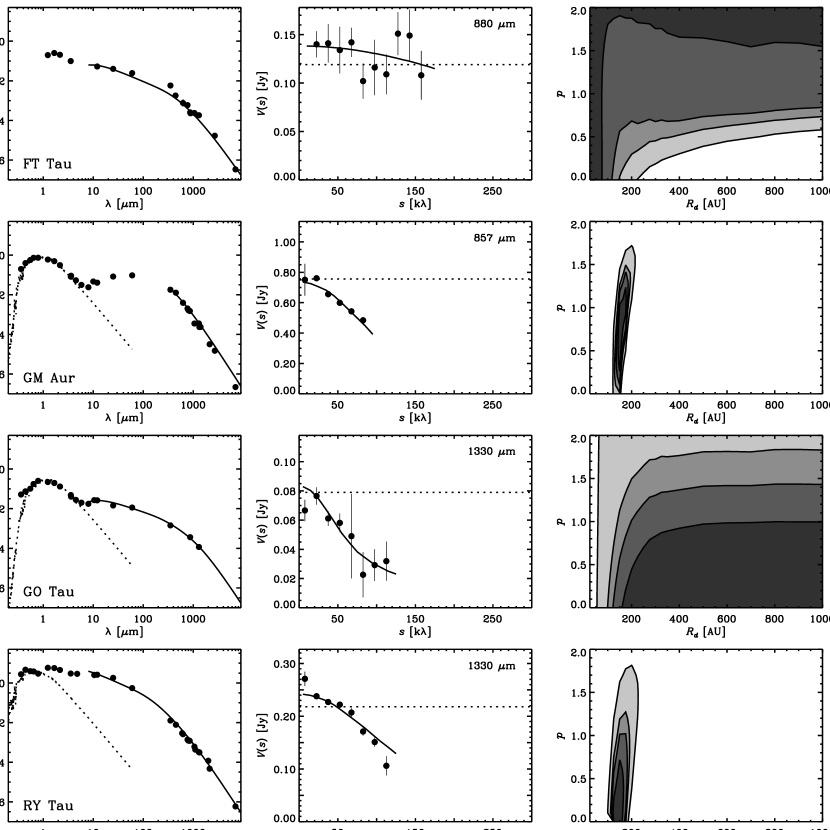
Figure 5: Same as Fig. 3.

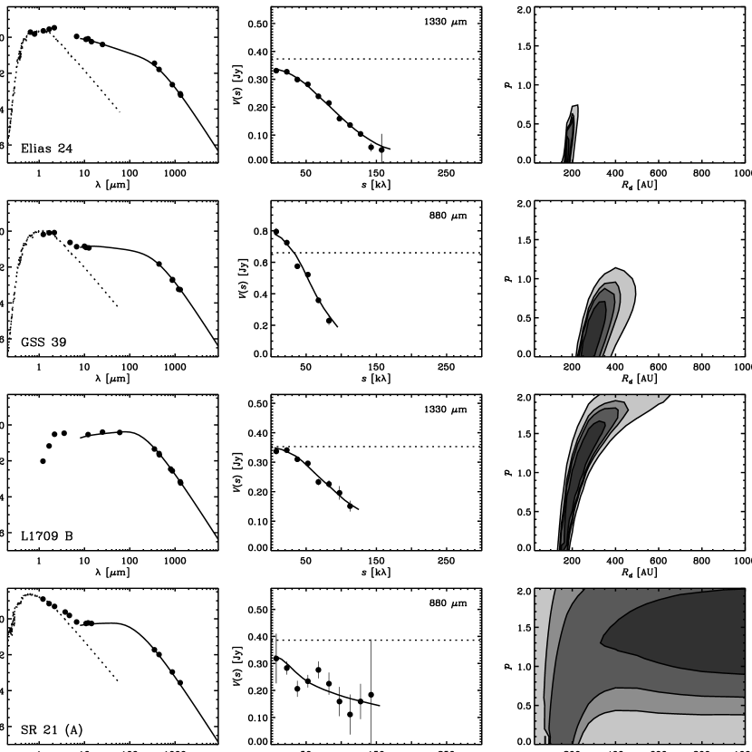
Figure 7: Same as Fig. 3.

Figure 9: Distributions of the parameters describing the radial variation of disk temperatures for this sample: the top panel for $\log{T_{1}}$, the temperature at 1 AU, and the bottom panel for $q$, the radial power-law index. The distributions were created to roughly account for parameter uncertainties as described in §4.1.1 for each measurement in Table 4. The bottom panel labels the idealized $q$ values for flared ($q\approx 0.43$) and flat ($q\approx 0.75$) disks.

Figure 10: A median temperature distribution for the sample. The datapoints correspond to sample median temperatures at representative radii determined from the best-fit {$T_{1}$, $q$} values in Table 4. Error bars show the first and third quartiles of the temperatures at each radius, meant to represent the range of $T_{r}$ in the sample. The dotted line gives the temperature profile constructed from the median values of {$T_{1}$, $q$}. The solid curve shows the distribution of the midplane disk temperature from a more detailed model (cf., D’Alessio et al., 2005), with star/disk parameters representative of the sample (see text). Such models exhibit temperature distributions which are approximately flat for small radii and flared for larger radii, as labeled here. A reminder at the top of the plot distinguishes the regions in the disk where the temperature distribution is actually measured (inner disk) or merely extrapolated (outer disk).

Figure 11: Distributions of the disk surface density profile parameters for this sample: the top panel for $\log{\Sigma_{5}}$, the surface density at 5 AU, and the bottom panel for $p$, the radial power-law index. The distributions were created as for Fig. 9 based on the best-fit values in Table 4. The top panel shows the 5 AU surface density for the minimum mass solar nebula (MMSN), and the bottom panel shows the power-law indices for both the MMSN and a steady viscous accretion disk.

Figure 12: A median surface density distribution for the sample. As in Fig. 10, the datapoints correspond to sample median surface densities at representative radii determined from the best-fit {$\Sigma_{5}$, $p$} values in Table 4. Error bars show the first and third quartiles of the surface densities at each radius, meant to represent the range of $\Sigma_{r}$ in the sample. The dotted line gives the surface density profile constructed from the median values of {$\Sigma_{5}$, $p$}. The solid curve shows the density distribution from a detailed model (cf., D’Alessio et al., 2005), with the same parameters as in Fig. 10 (see text). Such models have $\Sigma_{r}\propto r^{-1}$ and an exponential cut-off at large radii. The dot-dashed line marks the MMSN density distribution. A reminder at the top of the plot distinguishes the regions in the disk where $\Sigma_{r}$ is actually measured (outer disk) or merely extrapolated (inner disk).

Figure 13: Distributions of the outer disk radii, $R_{d}$, and total disk masses, $M_{d}$, for this sample, created as for those in Figs. 9 and 11 from the measurements in Table 4.

Figure 14: Distribution of the power-law index of the opacity spectrum, $\beta$, created as for Figs. 9, 11, and 13 from the values listed in Table 5. The value of $\beta$ for the ISM is marked with a dot-dashed vertical line.

Figure 15: Variations of the 850 $\mu$m flux densities (top left), mass accretion rates (top right; from the literature, see Table 3), outer radii (bottom left), and elliptical Gaussian FWHM (bottom right; determined from a fit to the C1 or C2 visibilities) with stellar age (see Table 3). Overlaid are the expected trends for two fiducial accretion disk models with $\alpha=0.01$ (solid) and $\alpha=0.001$ (dashed). Descriptions of the other parameters and the method of relating flat disk $R_{d}$ values with the accretion disk models are given in §5.1. The different symbols in the bottom right panel describing the FWHM correspond to two observing wavelengths used in this survey. The double accretion disk model curves also correspond to these two wavelengths, where the 1330 $\mu$m FWHM values are always slightly larger than at 880 $\mu$m. Typical systematic errors on stellar ages could be a factor of 2 or more for any individual object.

Figure 16: The sample median SED (top) and flux-normalized visibility profiles at 880 $\mu$m (middle) and 1330 $\mu$m (bottom) are shown to approximate the typical observables for a T Tauri disk. The error bars indicate the first and third quartiles at each wavelength or spatial frequency distance. The visibility profiles have their fluxes normalized at a spatial frequency distance $s\sim 20$ k$\lambda$. The data from individual disks are shown as small points. The contribution of a K7 stellar photosphere is shown as a dashed profile in the top SED panel. Overlaid on each panel are the same two fiducial accretion disk models shown in Figure 15 for $\alpha=0.01$ (solid) and $\alpha=0.001$ (dashed). These models were computed at the median age for the sample, $\sim$1 Myr.

Table 6: Literature Sources for SEDs

Object	References for $F_{\nu}$ at Various Wavelengths (in $\mu$m)
	8	10	12	25	60	350	450	600	800	850	1000	1300	2000	2700	7000
04158+2805	$\cdots$	$\cdots$	1	1	1	2	2	$\cdots$	$\cdots$	2	$\cdots$	3	$\cdots$	$\cdots$	$\cdots$
AA Tau	$\cdots$	4	5	5	5	6	6	$\cdots$	7	6	7	8	9	10	$\cdots$
CI Tau	$\cdots$	11	5	5	5	6	6	7	7	6	7	8	$\cdots$	10	12
DH Tau (A)	$\cdots$	$\cdots$	5	5	5	6	6	$\cdots$	13	6	$\cdots$	$\cdots$	$\cdots$	10	$\cdots$
DL Tau	14	$\cdots$	5	5	5	15	15	15, 7	7, 15	15	7, 15	8	9	10	12
DM Tau	$\cdots$	$\cdots$	$\cdots$	$\cdots$	$\cdots$	6	$\cdots$	7	7	6	7	8	9	10	12
DN Tau	$\cdots$	16	5	5	5	6	$\cdots$	$\cdots$	7	6	7	8	9	10	$\cdots$
DR Tau	14	11	5	5	5	15	6, 15	15	7, 15	15, 6	7, 15	8	9	$\cdots$	$\cdots$
FT Tau	$\cdots$	$\cdots$	5	5	5	6	6	7	7	6	7	8	$\cdots$	10	12
GM Aur	$\cdots$	$\cdots$	$\cdots$	$\cdots$	$\cdots$	6	17	7	7, 17	$\cdots$	7	8	9	18	12
GO Tau	14	16	5	5	5	6	$\cdots$	$\cdots$	$\cdots$	6	$\cdots$	8	$\cdots$	$\cdots$	$\cdots$
RY Tau	$\cdots$	11	5	5	5	15	15	15, 7	7, 15	15	7, 15	8	15, 9	$\cdots$	12
AS 205 (A)	19	19	5, 19	5	5	20	20	$\cdots$	21	20	21	22	$\cdots$	$\cdots$	$\cdots$
AS 209	$\cdots$	19	5	5	5	20	20	$\cdots$	$\cdots$	20	$\cdots$	22	$\cdots$	$\cdots$	$\cdots$
DoAr 25	$\cdots$	$\cdots$	$\cdots$	$\cdots$	$\cdots$	$\cdots$	23	$\cdots$	23	20	$\cdots$	22	$\cdots$	$\cdots$	$\cdots$
DoAr 44	$\cdots$	$\cdots$	24	24	25	$\cdots$	$\cdots$	$\cdots$	$\cdots$	20	$\cdots$	26	$\cdots$	$\cdots$	$\cdots$
Elias 24	$\cdots$	27	24, 28	24	$\cdots$	20	20	$\cdots$	$\cdots$	20	$\cdots$	22	$\cdots$	$\cdots$	$\cdots$
GSS 39	$\cdots$	27	29	$\cdots$	$\cdots$	$\cdots$	20	$\cdots$	$\cdots$	20	$\cdots$	22	$\cdots$	$\cdots$	$\cdots$
L1709 B	$\cdots$	$\cdots$	24	24	24	20	20, 23	$\cdots$	23	20	$\cdots$	22	$\cdots$	$\cdots$	$\cdots$
SR 21 (A)	$\cdots$	27	24, 28	$\cdots$		20	20	$\cdots$	$\cdots$	20	$\cdots$	22	$\cdots$	$\cdots$	$\cdots$
SR 24 (S)	$\cdots$	30	$\cdots$	30	$\cdots$	20	20	$\cdots$	$\cdots$	20	$\cdots$	26	$\cdots$	$\cdots$	$\cdots$
WaOph 6	31, 32	31	$\cdots$	31	31	$\cdots$	20	$\cdots$	$\cdots$	20	$\cdots$	22	$\cdots$	$\cdots$	$\cdots$
WSB 60	$\cdots$	33	33, 28	33	$\cdots$	20	20	$\cdots$	$\cdots$	20	$\cdots$	22	$\cdots$	$\cdots$	$\cdots$

Note. — References are as follows: 1 - Kenyon et al. (1990); 2 - M. C. Liu, private communication; 3 - Motte & André (2001); 4 - Metchev et al. (2004); 5 - Weaver & Jones (1992); 6 - Andrews & Williams (2005); 7 - Beckwith & Sargent (1991); 8 - Beckwith et al. (1990); 9 - Kitamura et al. (2002); 10 - Dutrey et al. (1996); 11 - Kenyon & Hartmann (1995); 12 - Rodmann et al. (2006); 13 - Jewitt (1994); 14 - Hartmann et al. (2005); 15 - Mannings & Emerson (1994); 16 - Simon & Prato (1995); 17 - Weintraub et al. (1989); 18 - Looney et al. (2000); 19 - Liu et al. (1996); 20 - Andrews & Williams, in preparation; 21 - Jensen et al. (1996); 22 - André & Montmerle (1994); 23 - Dent et al. (1998); 24 - IRAS Point Source Catalog; 25 - Clarke (1991); 26 - Nürnberger et al. (1998); 27 - Barsony et al. (2005); 28 - Bontemps et al. (2001); 29 - Lada & Wilking (1984); 30 - McCabe et al. (2006); 31 - Padgett et al. (2006); 32 - Gras-Velazquez & Ray (2005); 33 - Wilking et al. (1989).

References

- Adams et al. (1987) Adams, F. C., Lada, C. J., & Shu, F. H. 1987, ApJ, 312, 788
- Akeson et al. (1998) Akeson, R. L., Koerner, D. W., & Jensen, E. L. N. 1998, ApJ, 505, 358
- Akeson et al. (2002) Akeson, R. L., Ciardi, D. R., van Belle, G. T., & Creech-Eakman, M. J. 2002, ApJ, 566, 1124
- Akeson et al. (2005) Akeson, R. L., et al. 2005, ApJ, 622, 440
- Andrews & Williams (2005b) Andrews, S. M., & Williams, J. P. 2005, ApJ, 619, L175 (2005b)
- Andrews & Williams (2005) Andrews, S. M., & Williams, J. P. 2005, ApJ, 631, 1134
- André & Montmerle (1994) André, P., & Montmerle, T. 1994, ApJ, 420, 837
- Artymowicz & Lubow (1994) Artymowicz, P., & Lubow, S. H. 1994, ApJ, 421, 651
- Balbus & Hawley (1991) Balbus, S. A., & Hawley, J. F. 1991, ApJ, 376, 214
- Barsony et al. (2002) Barsony, M., Greene, T. P., & Blake, G. A. 2002, ApJ, 572, L75
- Barsony et al. (2003) Barsony, M., Koresko, C., & Matthews, K. 2003, ApJ, 591, 1064
- Barsony et al. (2005) Barsony, M., Ressler, M. E., & Marsh, K. A. 2005, ApJ, 630, 381
- Beckwith et al. (1990) Beckwith, S. V. W., Sargent, A. I., Chini, R. S., & Güsten, R. 1990, AJ, 99, 924
- Beckwith & Sargent (1991) Beckwith, S. V. W., & Sargent, A. I. 1991, ApJ, 381, 250
- Beckwith et al. (2000) Beckwith, S. V. W., Henning, T., & Nakagawa, Y. 2000, in Protostars and Planets IV, eds. V. Mannings, A. P. Boss, & S. S. Russell (Tucson: Univ. Arizona Press), 533
- Beichman et al. (1988) Beichman, C. A., Neugebauer, G., Habing, H. J., Clegg, P. E., & Chester, T. J. 1988, IRAS Catalogs and Atlases, Vol. 1, Explanatory Suppl. (Washington: NASA Scientific and Techn. Information Div.)
- Bontemps et al. (2001) Bontemps, S., et al. 2001, A&A, 372, 173
- Boss (1998) Boss, A. P. 1998, ApJ, 503, 923
- Boss (2005) Boss, A. P. 2005, ApJ, 629, 535
- Bouvier & Appenzeller (1992) Bouvier, J., & Appenzeller, I. 1992, A&AS, 92, 481
- Bouvier et al. (1995) Bouvier, J., Covino, E., Kovo, O., Martín, E. L., Matthews, J. M., Terranegra, L., & Beck, S. C. 1995, A&A, 299, 89
- Bouvier et al. (1999) Bouvier, J., et al. 1999, A&A, 349, 619
- Calvet et al. (2002) Calvet, N., D’Alessio, P., Hartmann, L., Wilner, D., Walsh, A., & Sitko, M. 2002, ApJ, 568, 1008
- Calvet et al. (2004) Calvet, N., Muzerolle, J., Briceño, C., Hernández, J., Hartmann, L., Saucedo, J. L., & Gordon, K. D. 2004, AJ, 128, 1294
- Calvet et al. (2005) Calvet, N., et al. 2005, ApJ, 630, L185
- Chiang & Goldreich (1997) Chiang, E. I., & Goldreich, P. 1997, ApJ, 490, 368
- Chiang & Goldreich (1999) Chiang, E. I., & Goldreich, P. 1999, ApJ, 519, 279
- Chiang et al. (2001) Chiang, E. I., Joung, M. K., Creech-Eakman, M. J., Qi, C., Kessler, J. E., Blake, G. A., & van Dishoeck, E. F. 2001, ApJ, 547, 1077
- Clarke (1991) Clarke, F. O. 1991, ApJS, 75, 611
- Clayton & Nittler (2004) Clayton, D. D., & Nittler, L. R. 2004, ARA&A, 42, 39
- Cutri et al. (2003) Cutri, R. M., et al. 2003, 2MASS All-Sky Catalog of Point Sources (Pasadena: IPAC)
- D’Alessio et al. (1998) D’Alessio, P., Cantó, J., Calvet, N., & Lizano, S. 1998, ApJ, 500, 411
- D’Alessio et al. (1999) D’Alessio, P., Calvet, N., Hartmann, L., Lizano, S., Cantó, J. 1999, ApJ, 527, 893
- D’Alessio et al. (2001) D’Alessio, P., Calvet, N., & Hartmann, L. 2001, ApJ, 553, 321
- D’Alessio et al. (2005) D’Alessio, P., Merín, B., Calvet, N., Hartmann, L., & Montesinos, B. 2005, Rev. Mexicana Astron. Astrofis., 41, 61
- D’Alessio et al. (2006) D’Alessio, P., Calvet, N., Hartmann, L., Franco-Hernández, R., & Servín, H. 2006, ApJ, 638, 314
- Dartois et al. (2003) Dartois, E., Dutrey, A., & Guilloteau, S. 2003, A&A, 399, 773
- de Geus et al. (1989) de Geus, E. J., de Zeeuw, P. T., & Lub, J. 1989, A&A, 216, 44
- Dent et al. (1998) Dent, W. R. F., Matthews, H. E., & Ward-Thompson, D. 1998, MNRAS, 301, 1049
- Dominik et al. (2006) Dominik, C., Blum, J., Cuzzi, J. N., & Wurm, G. 2006, in Protostars and Planets V, eds. B. Reipurth, D. C. Jewitt, & K. Keil (Tucson: Univ. Arizona Press), in press (astro-ph/0602617)
- Draine (2006) Draine, B. T. 2006, ApJ, 636, 1114
- Duchêne et al. (2003) Duchêne, G., Ménard, F., Stapelfeldt, K., & Duvert, G. 2003, A&A, 400, 559
- Dullemond et al. (2002) Dullemond, C. P., van Zadelhoff, G. J., & Natta, A. 2002, A&A, 389, 464
- Dullemond & Dominik (2004) Dullemond, C. P., & Dominik, C. 2004, A&A, 421, 1075
- Dullemond & Dominik (2005) Dullemond, C. P., & Dominik, C. 2005, A&A, 434, 971
- Dullemond et al. (2006) Dullemond, C. P., Hollenbach, D., Kamp, I., & D’Alessio, P. 2006, in Protostars and Planets V, eds. B. Reipurth, D. C. Jewitt, & K. Keil (Tucson: Univ. Arizona Press), in press (astro-ph/0602619)
- Durisen et al. (2005) Durisen, R. H., Cai, K., Mejía, A. C., & Pickett, M. K. 2005, Icarus, 173, 417
- Dutrey et al. (1996) Dutrey, A., Guilloteau, S., Duvert, G., Prato, L., Simon, M., Schuster, K., & Ménard, F. 1996, A&A, 309, 493
- Dutrey et al. (1998) Dutrey, A., Guilloteau, S., Prato, L., Simon, M., Duvert, G., Schuster, K., & Ménard, F. 1998, A&A, 338, L63
- Dutrey et al. (2003) Dutrey, A., Guilloteau, S., & Simon, M. 2003, A&A, 402, 1003
- Dutrey et al. (2006) Dutrey, A., Guilloteau, S., & Ho, P. T. P. 2006, in Protostars and Planets V, eds. B. Reipurth, D. C. Jewitt, & K. Keil (Tucson: Univ. of Arizona Press), in press
- Eisner et al. (2005) Eisner, J. A., Hillenbrand, L. A., White, R. J., Akeson, R. J., & Sargent, A. I. 2005, ApJ, 623, 952
- Elias (1978) Elias, J. H. 1978, ApJ, 224, 857
- Fischer & Valenti (2005) Fischer, D. A., & Valenti, J. 2005, ApJ, 622, 1102
- Ghez et al. (1993) Ghez, A. M., Neugebauer, G., & Matthews, K. 1993, AJ, 106, 2005
- Gras-Velazquez & Ray (2005) Gras-Velázquez, À., & Ray, T. P. 2005, A&A, 443, 541
- Greene & Meyer (1995) Greene, T. P., & Meyer, M. R. 1995, ApJ, 450, 233
- Guillot (2005) Guillot, T. 2005, Annu. Rev. Earth Planet. Sci., 33, 493
- Guilloteau & Dutrey (1998) Guilloteau, S., & Dutrey, A. 1998, A&A, 339, 467
- Guilloteau et al. (1999) Guilloteau, S., Dutrey, A., & Simon, M. 1999, A&A, 348, 570
- Gullbring et al. (1998) Gullbring, E., Hartmann, L., Briceño, C., & Calvet, N. 1998, ApJ, 492, 323
- Hamidouche et al. (2006) Hamidouche, M., Looney, L. W., & Mundy, L. G. 2006, ApJ, in press (astro-ph/0607232)
- Hartigan et al. (1995) Hartigan, P., Edwards, S., & Ghandour, L. 1995, ApJ, 452, 736
- Hartmann et al. (1998) Hartmann, L., Calvet, N., Gullbring, E., & D’Alessio, P. 1998, ApJ, 495, 385
- Hartmann et al. (2005) Hartmann, L., et al. 2005, ApJ, 629, 881
- Hartmann et al. (2006) Hartmann, L., D’Alessio, P., Calvet, N., & Muzerolle, J. 2006, ApJ, in press (astro-ph/0605294)
- Hayashi et al. (1985) Hayashi, C., Nakazawa, K., & Nakagawa, Y. 1985, in Protostars and Planets II, eds. D. C. Black, & M. S. Mathews (Tucson: Univ. Arizona Press), 1100
- Henning et al. (1995) Henning, T., Michel, B., & Stognienko, R. 1995, Planet. Space Sci., 43, 1333
- Henning & Stognienko (1996) Henning, T., & Stognienko, R. 1996, A&A, 311, 291
- Herbig & Bell (1988) Herbig, G. H., & Bell, K. R. 1988, Catalog of Emission-line Stars of the Orion Population (Santa Cruz: Lick Obs.)
- Herbst & Shevchenko (1999) Herbst, W., & Shevchenko, V. S. 1999, AJ, 118, 1033
- Hildebrand (1983) Hildebrand, R. 1983, QJRAS, 24, 267
- Ho et al. (2004) Ho, P. T. P., Moran, J. M., & Lo, K. Y. 2004, ApJ, 616, L1
- Hueso & Guillot (2005) Hueso, R., & Guillot, T. 2005, A&A, 442, 703
- Inaba et al. (2003) Inaba, S., Wetherill, G. W., & Ikoma, M. 2003, Icarus, 166, 46
- Itoh et al. (2005) Itoh, Y., et al. 2005, ApJ, 620, 984
- Jensen et al. (1996) Jensen, E. L. N., Mathieu, R. D., & Guller, G. A. 1996, ApJ, 458, 312
- Jewitt (1994) Jewitt, D. C. 1994, AJ, 108, 661
- Johnstone et al. (1998) Johnstone, D., Hollenbach, D., & Bally, J. 1998, ApJ, 499, 758
- Keene & Masson (1990) Keene, J., & Masson, C. R. 1990, ApJ, 355, 635
- Kenyon & Hartmann (1987) Kenyon, S. J., & Hartmann, L. 1987, ApJ, 323, 714
- Kenyon et al. (1990) Kenyon, S. J., Hartmann, L. W., Strom, K. M., & Strom, S. E. 1990, AJ, 99, 869
- Kenyon & Hartmann (1995) Kenyon, S. J., & Hartmann, L. 1995, ApJS, 101, 117
- Kitamura et al. (2002) Kitamura, Y., Momose, M., Yokogawa, S., Kawabe, R., Tamura, M., & Ida, S. 2002, ApJ, 581, 357
- Koerner et al. (1993) Koerner, D. W., Sargent, A. I., & Beckwith, S. V. W. 1993, Icarus, 106, 2
- Koerner & Sargent (1995) Koerner, D. W., & Sargent, A. I. 1995, AJ, 109, 2138
- Krügel & Siebenmorgen (1994) Krügel, E., & Siebenmorgen, R. 1994, A&A, 288, 929
- Kuchner (2004) Kuchner, M. J. 2004, 612, 1147
- Kurucz (1993) Kurucz, R. L. 1993, Solar Abundance Model Atmospheres, Kurucz CD-Rom No. 19
- Lada & Wilking (1984) Lada, C. J., & Wilking, B. A. 1984, ApJ, 287, 610
- Lay et al. (1994) Lay, O. P., Carlstrom, J. E., Hills, R. E., & Phillips, T. G. 1994, ApJ, 434, L75
- Lay et al. (1997) Lay, O. P., Carlstrom, J. E., & Hills, R. E. 1997, ApJ, 489, 917
- Leinert et al. (1993) Leinert, C. et al. 1993, A&A, 278, 129
- Lin & Bodenheimer (1982) Lin, D. N. C., & Bodenheimer, P. 1982, ApJ, 262, 768
- Lissauer (1987) Lissauer, J. J. 1987, Icarus, 69, 249
- Liu et al. (1996) Liu, M. C., et al. 1996, ApJ, 461, 334
- Looney et al. (2000) Looney, L. W., Mundy, L. G., & Welch, W. J. 2000, ApJ, 529, 477
- Looney et al. (2003) Looney, L. W., Mundy, L. G., & Welch, W. J. 2003, ApJ, 592, 255
- Lunine et al. (2004) Lunine, J. I., Coradini, A., Gautier, D., Owen, T. C., & Wuchterl, G. 2004, in Jupiter: the Planet, Satellites, and Magnetosphere, eds. F. Baganal, T. E. Dowling, & W. B. McKinnon (Cambridge: Cambridge Univ. Press), 19
- Luu & Jewitt (2002) Luu, J. X., & Jewitt, D. C. 2002, ARA&A, 40, 63
- Lynden-Bell & Pringle (1974) Lynden-Bell, D., & Pringle, J. E. 1974, MNRAS, 168, 603
- Mannings & Emerson (1994) Mannings, V., & Emerson, J. P. 1994, MNRAS, 267, 361
- Marcy et al. (2000) Marcy, G. W., Cochran, W. D., & Mayor, M. 2000, in Protostars and Planets IV, eds. V. Mannings, A. P. Boss, & S. S. Russell (Tucson: Univ. Arizona Press), 1285
- Mathis (1990) Mathis, J. S. 1990, ARA&A, 28, 37
- McCabe et al. (2003) McCabe, C., Duchêne, G., & Ghez, A. M. 2003, ApJ, 588, L113
- McCabe et al. (2006) McCabe, C., Ghez, A. M., Prato, L., Duchêne, G., Fischer, R. S., & Telesco, C. 2006, ApJ, 636, 932
- McCaughrean & O’Dell (1996) McCaughrean, M. J., & O’Dell, C. R. 1996, AJ, 111, 1977
- Metchev et al. (2004) Metchev, S. A., Hillenbrand, L. A., & Meyer, M. R. 2004, ApJ, 600, 435
- Miyake & Nakagawa (1993) Miyake, K., & Nakagawa, Y. 1993, Icarus, 106, 20
- Mora et al. (2001) Mora, A., et al. 2001, A&A, 378, 116
- Motte & André (2001) Motte, F., & André, P. 2001, A&A, 365, 440
- Mundy et al. (1996) Mundy, L. G., et al. 1996, ApJ, 464, L169
- Muzerolle et al. (1998) Muzerolle, J., Hartmann, L., & Calvet, N. 1998, AJ, 116, 2965
- Muzerolle et al. (2003a) Muzerolle, J., Hillenbrand, L., Calvet, N., Briceño, C., & Hartmann, L. 2003, ApJ, 592, 266 (2003a)
- Muzerolle et al. (2003b) Muzerolle, J., Calvet, N., Hartmann, L., & D’Alessio, P. 2003, ApJ, 597, L149 (2003b)
- Natta et al. (2004) Natta, A., Testi, L., Neri, R., Shepherd, D. S., & Wilner, D. J. 2004, A&A, 416, 179
- Natta et al. (2006a) Natta, A., Testi, L., & Randich, S. 2006, A&A, 452, 245
- Natta et al. (2006b) Natta, A., Testi, L., Calvet, N., Henning, T., Waters, R., & Wilner, D. 2006, in Protostars and Planets V, eds. B. Reipurth, D. C. Jewitt, & K. Keil (Tucson: Univ. Arizona Press), in press (astro-ph/0602041) (2006b)
- Nürnberger et al. (1998) Nürnberger, D., Brandner, W., Yorke, H. W., & Zinnecker, H. 1998, A&A, 330, 549
- O’Sullivan et al. (2005) O’Sullivan, M., Truss, M., Walker, C., Wood, K., Matthews, O., Whitney, B., & Bjorkman, J. E. 2005, MNRAS, 358, 632
- Padgett et al. (2006) Padgett, D. L., et al. 2006, ApJ, 645, 1283
- Pollack et al. (1994) Pollack, J. B., Hollenbach, D., Beckwith, S., Simonelli, D. P., Roush, T., & Fong, W. 1994, ApJ, 421, 615
- Pollack et al. (1996) Pollack, J. B., Hubickyj, O., Bodenheimer, P., Lissauer, J. J., Podolak, M., & Greenzweig, Y. 1996, Icarus, 124, 62
- Prato et al. (2003) Prato, L., Greene, T. P., & Simon, M. 2003, ApJ, 584, 853
- Pringle (1981) Pringle, J. E., 1981, ARA&A, 19, 137
- Qi et al. (2003) Qi, C., Kessler, J. E., Koerner, D. W., Sargent, A. I., & Blake, G. A. 2003, ApJ, 597, 986
- Qi et al. (2004) Qi, C., et al. 2004, ApJ, 616, L7
- Qi et al. (2006) Qi, C., et al. 2006, ApJ, 636, L157
- Ratzka et al. (2005) Ratzka, T., Koehler, R., & Leinert, C. 2005, A&A, 437, 611
- Raymond et al. (2005) Raymond, S. N., Quinn, T., & Lunine, J. I. 2005, ApJ, 632, 670
- Reipurth & Zinnecker (1993) Reipurth, B., & Zinnecker, H. 1993, A&A, 278, 81
- Rodmann et al. (2006) Rodmann, J., Henning, T., Chandler, C. J., Mundy, L. G., & Wilner, D. J. 2006, A&A, 446, 211
- Santos et al. (2001) Santos, N. C., Israelian, G., & Mayor, M. 2001, A&A, 373, 1019
- Shakura & Sunyaev (1973) Shakura, N. I., & Sunyaev, R. A. 1973, A&A, 24, 337
- Simon et al. (1995) Simon, M., et al. 1995, ApJ, 443, 625
- Simon & Prato (1995) Simon, M., & Prato, L. 1995, ApJ, 450, 824
- Simon et al. (2000) Simon, M., Dutrey, A., & Guilloteau, S. 2000, ApJ, 545, 1034
- Takeuchi & Lin (2005) Takeuchi, T., & Lin, D. N. C. 2005, ApJ, 623, 482
- Testi et al. (2001) Testi, L., Natta, A., Shepherd, D. S., & Wilner, D. J. 2001, ApJ, 554, 1087
- Testi et al. (2003) Testi, L., Natta, A., Shepherd, D. S., & Wilner, D. J. 2003, A&A, 403, 323
- Thamm et al. (1994) Thamm, E., Steinacker, J., & Henning, T. 1994, A&A, 287, 493
- Udry et al. (2006) Udry, S., Fischer, D. A., & Queloz, D. 2006, in Protostars and Planets V, eds. B. Reipurth, D. C. Jewitt, & K. Keil (Tucson: Univ. Arizona Press), in press
- Valenti et al. (1993) Valenti, J. A., Basri, G., & Johns, C. M. 1993, AJ, 106, 2024
- Vicente & Alves (2005) Vicente, S. M., & Alves, J. 2005, A&A, 441, 195
- Weaver & Jones (1992) Weaver, W. B., & Jones, G. 1992, ApJS, 78, 239
- Weidenschilling (1977) Weidenschilling, S. J. 1977, Ap&SS, 51, 153
- Weingartner & Draine (2001) Weingartner, J. C., & Draine, B. T. 2001, ApJ, 548, 296
- Weintraub et al. (1989) Weintraub, D. A., Sandell, G., & Duncan, W. D. 1989, ApJ, 340, L69
- White & Hillenbrand (2004) White, R. J., & Hillenbrand, L. A. 2004, ApJ, 616, 998
- Wilking et al. (1989) Wilking, B. A., Lada, C. J., & Young, E. T. 1989, ApJ, 340, 823
- Wilking et al. (2005) Wilking, B. A., Meyer, M. R., Robinson, J. G., & Greene, T. P. 2005, AJ, 130, 1733
- Wilner et al. (1996) Wilner, D. J., Ho, P. T. P., & Rodríguez, L. F. 1996, ApJ, 470, L117
- Wilner et al. (2000) Wilner, D. J., Ho, P. T. P., Kastner, J. H., & Rodríguez, L. F. 2000, ApJ, 534, L101
- Wilner et al. (2003) Wilner, D. J., Bourke, T. L., Wright, C. M., Jørgensen, J. K., van Dishoeck, E. F., & Wong, T. 2003, ApJ, 596, 597
- Wilner et al. (2005) Wilner, D. J., D’Alessio, P., Calvet, N., Claussen, M. J., & Hartmann, L. 2005, ApJ, 626, L109
- Wright (1987) Wright, E. L. 1987, ApJ, 320, 818
- Youdin & Shu (2002) Youdin, A. N., & Shu, F. H. 2002, ApJ, 580, 494