The HgMn Binary Star $\phi$ Herculis: Detection and Properties of the Secondary and Revision of the Elemental Abundances of the Primary

Abstract

Observations of the Mercury-Manganese star $\phi$ Her with the Navy Prototype Optical Interferometer (NPOI) conclusively reveal the previously unseen companion in this single-lined binary system. The NPOI data were used to predict a spectral type of A8V for the secondary star $\phi$ Her B. This prediction was subsequently confirmed by spectroscopic observations obtained at the Dominion Astrophysical Observatory. $\phi$ Her B is rotating at 50 $\pm$ 3 km s^-1, in contrast to the 8 km s^-1 lines of $\phi$ Her A. Recognizing the lines from the secondary permits one to separate them from those of the primary. The abundance analysis of $\phi$ Her A shows an abundance pattern similar to those of other HgMn stars with Al being very underabundant and Sc, Cr, Mn, Zn, Ga, Sr, Y, Zr, Ba, Ce, and Hg being very overabundant.

1 Introduction

The Mercury-Manganese (HgMn) stars are a class of non-magnetic peculiar main sequence B type stars with effective temperatures between 10500 K and 15000 K. Their members show a wide variety of abundance anomalies with both depletions (e.g., N, Roby et al., 1999) and enhancements (Hg: Leckrone et al. 1991; Mn: Woolf & Woolf 1976) and tend to be slow rotators relative to their normal analogs. Enhancements of some elements may be as large as 10⁵ times the solar abundances (Preston, 1974). References to many recent abundance studies of HgMn stars can be found by consulting, e.g., Adelman et al. (2004b, 2006). These abundance anomalies are thought to be produced in an extremely hydrodynamically stable environment from the separation of elements by radiatively-driven diffusion and gravitational settling (Michaud, 1970). Woolf & Lambert (1999a) discovered three young HgMn stars in the Orion OB1 association. Two of these stars are members of the 1.7 Myr old OB1b sub-association which indicates how soon after the ZAMS such stars can be detected. The HgMn stars are important laboratories for studying stellar hydrodynamical effects. With results from many stars one can study the dependence of the elemental abundances on stellar parameters and make comparisons with theoretical predictions (Adelman, Gulliver & Rayle, 2001).

$\phi$ Herculis (HD 145389, HR 6023, V=4.23, $\alpha_{2000}=16^{\rm h}08^{\rm m}46^{\rm s}$, $\delta_{2000}=44\arcdeg\ 56^{\prime}$ 06”) is a HgMn star whose peculiar spectrum was noted in the Henry Draper catalog (Cannon & Pickering, 1921) with an inverse dispersion of 159 Å mm^-1. As most HgMn stars can only be found on higher resolution spectra, this indicates that $\phi$ Her is a star strongly showing the HgMn phenomena. The Henry Draper catalog entry noted that the Ca II K line was nearly as strong as in $\alpha$ Canis Majoris. The excess in manganese was noted by Morgan (1933). Osawa (1965) identified it as a HgMn star. It is also a single-lined spectroscopic binary (Aikman, 1976; Babcock, 1971), but the secondary has eluded detection until now. Mason et al. (1999) list $\phi$ Her as a Hipparcos binary which was not resolved by speckle interferometry although an orbit based on the photocenter motion was computed (Lindegren et al., 1997). Adelman et al. (2001) performed the most recent spectroscopic analysis of $\phi$ Her A with S/N $\geq$ 200 Reticon and CCD spectrograms. Commencing in 1997 interferometric observations of $\phi$ Her with the Navy Prototype Optical Interferometer (NPOI, Armstrong et al., 1998) were made as part of a program to observe binaries in the catalog of Batten et al. (1989). These were spectroscopic binaries selected by one of us (Hummel) whose orbits were expected to be resolved by the NPOI. Observations with the NPOI continued through 2005 June, and the secondary was clearly detected in the visibility data (Zavala et al., 2004). The interferometric detection of the secondary allowed us to predict the secondary’s spectral type. This was an important clue to the detection of the secondary’s lines. They are consistent with such a spectral type using observations obtained at the Dominion Astrophysical Observatory.

In this paper we describe the interferometric and spectroscopic observations which for the first time reveal the true nature of the secondary star of $\phi$ Her. The current study found some broad-lines from the secondary. Now we must correct for the contributions of the secondary in determining the properties of the primary star. These results show how the combination of interferometric and spectroscopic data allows for a single-lined binary to become a double-lined system, and hence improve our knowledge of the system.

2 Observations and Data Reduction

Both optical interferometric and spectroscopic data contributed to this study. We first consider the reduction of the data separately, and in §3 apply the two together to test the prediction of the secondary star’s spectral type and impact on $\phi$ Her as a chemically peculiar star.

2.1 NPOI Observations

$\phi$ Her was observed with the NPOI on 25 different epochs from 1997 April 19 to 2005 June 16. Armstrong et al. (1998) describe the NPOI in detail. Here we present a brief description of the instrument. The NPOI functions as a two to six element optical interferometer. The individual elements are siderostats with a 35 cm unvignetted aperture. The siderostats feed the light into evacuated pipes which send the light to a beam combining optical table. The pipes cause a stop-down of the effective aperture to 12 cm. Varying path length delays are removed by the use of Fast Delay Line (FDL) carts which are also contained in evacuated pipes. The FDL’s move continuously to adjust for the changing delay caused by a varying projected baseline length due to the Earth’s rotation. The light from the individual siderostats is combined on an optical bench to produce interference fringes. To provide an analogy to radio interferometry, the FDL’s and the beam combining table serve as the NPOI’s correlator. After combination spectrometers disperse the light which is collected onto lenslet arrays. These arrays feed the light to banks of avalanche photo diodes (APD) via fiber optic cables.

NPOI observations before 2001 used 32 channels across a 4500-8500Å bandwidth. The 2004 and 2005 observations spanned 5500-8500Å and used 16 channels. Table 1 provides a log of the NPOI observations. The change in number of spectral channels and wavelength coverage was required due to an improvement in the NPOI’s beam combination instrumentation. These changes allowed for the detection of multiple baselines on a single spectrometer, increasing the number of available baselines and thereby improving the NPOI’s ability to synthesize a filled aperture. The additional baselines more than offset the reduced 16 channel spectral resolution. See Fig. 1 for an example of the increased sampling in the uv plane enabled by the 8 baselines of the 2004 July 07 observation compared to the earlier observations. Several epochs in 2004 did not take full advantage of this capability (e.g., those with 3 siderostats). These observations were conducted as part of a stellar multiplicity survey which necessitated the use of only two baselines (Hutter et al., 2005). Details regarding the improvements which apply to the 2004 and 2005 observations can be found in Hummel et al. (2003) and Benson et al. (2003). For the 1999 and earlier observations see Benson et al. (1997) for instrument details.

Observations of the target star $\phi$ Her are interspersed with observations of the calibrator star $\tau$ Her. $\tau$ Her is located 2.4^∘ from $\phi$ Her, has a V magnitude of 3.89 (Hoffleit & Jaschek, 1982), and is a B5IV standard in the Revised MK system (Morgan & Keenan, 1973). During an observation of either $\phi$ Her or $\tau$ Her data are recorded every 2 msec. The 2 msec data are then averaged to produce points every 1 second. Data reduction was performed using C. A. Hummel’s OYSTER software package. Data points were initially flagged on the basis of several factors. Outlier points in delay residuals, seeing indicators, photon rates and visibilities were removed. The 1 second data points were then averaged to produce squared visibility data for each 30 seconds (a “scan”) taken of the calibrator and target star. These $V^{2}$ data contain an additive bias term and this bias was subtracted using the method described in Hummel et al. (2003) and Wittkowski et al. (2001).

Calibration is performed using the expected angular diameter of the calibrator star $\tau$ Her. The color and apparent magnitude of a star can be used to estimate the uniform disk angular diameter (Mozurkewich et al., 1991; White & Feierman, 1987). Using the R$-$I color of $\tau$ Her this diameter is estimated to be 0.28 mas. A multiplicative factor is then determined for each spectral channel so that the observed, bias corrected, $V^{2}$ data of the calibrator are brought inline with the theoretical expectation. This same calibration factor is then applied to the observed, bias corrected, $V^{2}$ data of $\phi$ Her. Calibration factors were determined versus time, in the manner described for NPOI data in Hummel et al. (1998).

2.2 DAO Spectroscopy

Our elemental analysis of $\phi$ Her A is an extension and modest revision of that of Adelman et al. (2001) who obtained Reticon and CCD exposures with the long camera of Coudé spectrograph of the 1.22-m telescope of the Dominion Astrophysical Observatory. Seven new spectra were obtained with the SITe4 CCD. The four centered at $\lambda$4864, $\lambda$5002, $\lambda$5140, and $\lambda$5278 are in the second order with a wavelength range of 147 Å and a two pixel resolution of 0.072 Å. Those centered at $\lambda$6562 and $\lambda$8556 are first order exposures with a wavelength range of 294 Å and a two pixel resolution of 0.144 Å. The spectrum centered at $\lambda$4340 with a wavelength range of 394 Å and a two pixel resolution of 0.195 Å was a short camera exposure which was used to extract the H$\gamma$ profile. The signal-to-noise ratios are respectively, 340, 300, 350, 370, 330, 460, and 250 at the continuum level. No measurements were made in regions of very heavy telluric contamination.

The analysis techniques are very similar to those of Adelman et al. (2001). The stellar exposures were flat fielded with the exposures of an incandescent lamp which was placed in the Coudé mirror train. The separation of the light of a desired order involved both optical coatings of the Coudé mirror train and glass photographic filters. To simulate the effects of the secondary mirror, a central stop was used. The one-dimensional scattered light corrected spectra were extracted using the program CCDSPEC (Gulliver & Hill 2002).

3 Detection of the Secondary

3.1 Interferometry

As a single lined spectroscopic binary (SB1) one could assume that the secondary star was at least one magnitude fainter than $\phi$ Her A (Heintz, 1978). Other than that not much else was known of $\phi$ Her B. There was a suggestion that the secondary could be a white dwarf (Stickland & Dworetsky, 1980). Fortunately optical interferometry allows the detection of secondary stars approximately three magnitudes fainter than the primary. $\phi$ Her was observed with the NPOI as part of a program to detect the secondary stars in SB1 systems selected from Batten et al. (1989). Early observations with the NPOI easily revealed the characteristic oscillation (Pan et al., 1992) of a binary star in the squared visibilities of $\phi$ Her. Fig. 2 shows an example of the calibrated $V^{2}$ data versus wavelength for $\phi$ Her obtained on 1998 May 16.

With the calibrated $V^{2}$ data we can now estimate the separation $\rho$ and position angle $\theta$ of the binary for each night. The individual $\rho$ and $\theta$ values are then used to determine the seven orbital elements as for visual and speckle binaries (Heintz, 1978). With the orbital elements we can use the visibility data from all observations and fit for the magnitude differences. Initial guesses for the stellar diameters and the magnitude differences are needed for the initial fits to $\rho$ and $\theta$ for individual nights. The primary’s spectral type and parallax can be used to estimate a diameter for the primary. With a Hipparcos (Perryman et al., 1997) parallax of 14.27 $\pm$ 0.52 mas a B8V star with a 3.0 R_⊙ radius (Cox, 2000) would have an angular diameter of 0.4 mas. The depth of the minimum $V^{2}$ is used to provide an estimate of the magnitude difference. Assuming both stars are on the main sequence we use the magnitude difference to estimate the secondary’s spectral type and diameter using Cox (2000). If both stars are on the main sequence we assume that $\phi$ Her B’s diameter is less than the diameter of A.

Fig. 3 shows an example of the final result for these fits. Six scans are shown for the 2004 July 31 NPOI data. The large panels show the calibrated $V^{2}$ as open circles with the model shown as a dotted line. The small lower panels depict the residuals from the model fit. The residuals are larger at the blue end which is expected due to the NPOI’s lower blue sensitivity relative to the red channels. In Table 2 we show the relative astrometric results for $\phi$ Her for all the NPOI observations. These relative astrometric solutions were used to solve for the orbital elements which are shown in Table 3.

A combined solution of the orbital elements using the NPOI astrometric positions and the single lined radial velocity curve of Aikman (1976) was performed. An initial conservative estimate of the error of the astrometric results were the positions and orientations of the CLEAN beam, an elliptical Gaussian fitted to the FWHM of the dirty beam (Högbom, 1974; Cornwell et al., 1999). This combined radial velocity and astrometric solution resulted in a reduced chi squared of 3.4. The individual reduced chi-squared using only the astrometric data was 0.3, and using only the radial velocity data was 5.5. We elected to reduce the error ellipses of the astrometric results and increase the error estimates for the radial velocity data. The final error ellipses shown in Table 2 have the dimensions of one-third of the CLEAN beam, and we increased the error estimates on the radial velocity data by a factor of $\sqrt{5}$. The subsequent orbital elements we fit have a reduced chi squared of 0.8 and are shown in Table 3. The orbit overlaid on the astrometric results is shown in Fig. 4 and the radial velocity data and residuals are shown in Fig. 5. We also plot the observed minus calculated values for the separation and position angle contained in Table 2 and these are shown in Fig. 6. The orbital elements in Table 3 are significantly different from the Hipparcos derived orbit (Hartkopf, Mason & Worley, 2001; Lindegren et al., 1997), and we did not incorporate the Hipparcos orbital elements in our solution.

The magnitude difference was the key to our prediction of the secondary spectral type, and we now consider the significance of that prediction. The data were taken over several years with changes to the instrument configuration (see §2.1) so first we consider the magnitude difference results for the individual calendar years of our observations. Table 4 contains the results of fits to the magnitude difference at 5500Å and 7000Å for the 5 years for which the NPOI observed $\phi$ Her. Fig. 7 illustrates these results with the red points used for the 1997$-$1999 observations and blue for the 2004$-$2005 observations. The scatter in Fig. 7 for the five different years of $\Delta$mag(7000Å) is larger than our error bars. Also, if we ignore the one result for 1999 as an outlier the 2004 and 2005 observations suggest a smaller $\Delta$mag(7000Å) compared to the 1997 and 1998 data. We decided to be conservative and use the maximum net extent of the 1$\sigma$ error bars in Fig. 7 to determine the magnitude differences and errors as: $\Delta$mag(5500Å) = 2.57 $\pm$ 0.05 and $\Delta$mag(7000Å) = 2.39 $\pm$ 0.05. The NPOI generally has a better sensitivity in the red as opposed to the blue end and we expect that systematic effects ultimately limit our errors to the level of $\pm$ 5% for the magnitude difference independent of wavelength. Recent tests, conducted after these observations, show that our wavelength calibration for the 2005 observations may have been off by 2 to 8 nm in several channels. Residual calibration errors may also contribute to the error budget. Although these systematics are difficult to quantify Fig. 7 shows that across 7 years and with a change to the NPOI beam combination and fringe detection equipment the final error of $\pm$ 5% in magnitudes seems rather good. With a magnitude difference of approximately 2.6 in V an error of $\pm$ 0.05 magnitudes corresponds to an error in the measured squared visibilities of less than 3%.

The magnitude differences of 2.57 at 5500Å and 2.39 at 7000Å (V and R bands, respectively) allowed us to predict the secondary’s spectral type as A8, using Table 15.7 of Cox (2000) assuming both stars are on the main sequence. Using the same table in Cox (2000) we see that the magnitude differences in V for a B8V$+$A5V binary is 2.2 and for a B8V$+$F0V binary it is 3.0. Both of these magnitude differences are at the 7$\sigma$ level for our NPOI results. This illustrates the NPOI’s capability to determine the the spectral type of the secondary of $\phi$ Her at the level of a few spectral subtypes.

Using the Hipparcos parallax and the orbital elements in Table 3 we determined the sum of the masses to be 4.7 $\pm$ 0.6 M_⊙. The dominant source of error in the sum of the masses is the uncertainty of the parallax. If the parallax were perfectly known we would know the mass sum to approximately 3%. The diameters used for $\phi$ Her A and B in our model fits are listed in Table 3 but we did not attempt to fit a diameter for either star. The expected diameters for the two components from Cox (2000) are too small to resolve with the NPOI configurations used in this study.

Using the mass sum from the dynamical parallax and the mass function of Aikman (1976) of 5.4$\times$10^-4 we can estimate the individual stellar masses. This method gives 3.6 and 1.1 M_⊙ respectively for the primary and secondary. These masses are too large for a B8V and too small for an A8V (Andersen, 1991). Using the tight mass$-$luminosity relationship and a bolometric correction of $-$0.75 for the primary we expect a B8V to have a mass closer to 3.1 M_⊙ which raises the secondary mass to 1.6 M_⊙. Clearly a precise determination of the stellar masses is not possible in this study of $\phi$ Her.

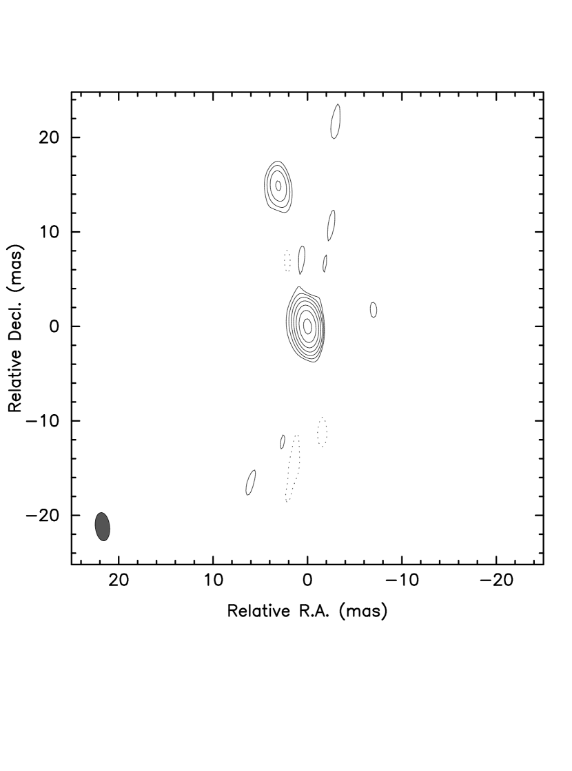
Figure 8: Image of $\phi$ Her on 2005 May 24 with a separation of 15 mas between components. Contour levels are -1.28, 1.28, 2.55, 5.1, 10.2, 20.4, 40.8 and 81.6% of map peak. The restoring beam is shown in the lower left hand corner and has dimensions of 3.01 $\times$ 1.53 mas with a position angle of 6.52^∘.

An image of $\phi$ Her produced from the 2005 May 24 NPOI observation is shown in Fig. 8. The image was produced in DIFMAP (Shepherd, 1997; Shepherd, Pearson & Taylor, 1994) using the CLEAN algorithm (Högbom, 1974) to remove the effects of irregular sampling in the uv plane (Fig. 1) to produce an image of the source. CLEAN requires as input the complex visibility (Thompson, Moran & Swenson, 1999)

$$V\equiv|V|e^{i\phi}$$ (1)

where $|V|$ is the visibility amplitude on a baseline and $\phi$ is the phase on that baseline. By taking the square root of the NPOI $V^{2}$ values and solving for the baseline phase with the requirement that the same closure phase is maintained we obtain the inputs required for CLEAN (Hummel et al., 2003). One limitation to this procedure is the requirement for at least three baselines which form a closure phase (Jennison, 1958) be present in the data. Thus the two baseline observations of $\phi$ Her do not allow us to form an image of the binary.

3.2 Spectroscopy

The spectra were rectified using the interactive computer graphics program REDUCE (Hill, Fisher & Pockert 1982). Gaussian profiles corresponding to v sin i = 8.0 km s^-1, the value found by Adelman et al. (2001), were fit through most of the metal line profiles as the spectra were measured with VLINE which is part of the REDUCE package. But a few lines were found corresponding to a rotational velocity of about 50 km s^-1. Rotational profiles were fit to these lines which must belong to the secondary, $\phi$ Her B. Thus $\phi$ Her now can be considered a double-lined spectroscopic binary.

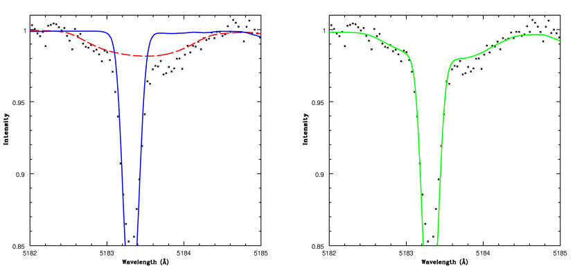
Figure 9: Left panel shows our observed spectra (x) overlaid on normalized synthetic spectra for $\phi$ Her A (blue solid line) and $\phi$ Her B (red long dashed line) We can see the primary and secondary components of Mg I (2) $\lambda$ 5183.6042. In the right panel we again show our data but now we overlay a line representing the summed synthetic spectra of $\phi$ Her A and B. Further information on the epoch of observation is available in Table 5.

Measuring these features is not trivial. It would be difficult to find them if the S/N ratios were much less than 300 at the resolution of the DAO long Coudé camera. Due to their shallow line depths, which are at most about 3% below the continuum level, parts of their profiles can be poorly defined. The resolution of our spectra is more than adequate to find them. Some lines of $\phi$ Her B which are weaker than those detected might have been partially removed by the rectification process while others are lost in the continuum noise. A search of the spectra of Adelman et al. (2001) did not reveal any additional candidates. Going to even higher S/N and to the red of $\lambda$5300 where the secondary contributes a greater percentage of light is the mostly likely way to find other lines in regions without telluric contamination. A list of those whose equivalent widths were greater than 10 mÅ and whose profiles are sufficiently well defined for radial velocity measurements is given in Table 5. Three of them are illustrated in Fig. 9. The lines of $\phi$ Her B are about 2 Å wide while those due to the primary are much narrower. The synthetic spectrum in Fig. 9 was produced using a vsin(i) of 50 km sec^-1. We estimate the uncertainty in vsin(i) for $\phi$ Her B as $\pm$ 3 km sec^-1 based on the 5 km sec^-1 error in the measured widths and the non-Gaussian line profiles.

To identify the stellar lines we used the general references A Multiple Table of Astrophysical Interests (Moore 1945) and Wavelengths and Transition Probabilities for Atoms and Atomic Ions, Part 1 (Reader & Corliss 1980) as well as references for specific atomic species (see Adelman et al. 2001). Zn II was the only new species we found. The rest of the lines belong to those species found by Adelman et al. (2001). For many species we found new lines to analyze. We were only able to identify the strongest lines in the $\lambda$8556 spectrogram.

We averaged the radial velocities for epochs 2004 Jun 10 and 2004 Jul 28, and plotted these averaged velocities with the epoch 2005 Jun 24 observation in Fig. 10. Using the averaged radial velocities from Table 5 results in a negligible improvement to the reduced chi-squared. In §3.1 we noted the difficulty in establishing a firm mass estimate. The uncertainties in the radial velocities of $\phi$ Her B do not provide a firm constraint on the velocity semi-amplitude. We note that our measured velocities are consistent with the prediction using the orbital elements in Table 3.

4 A New Look at $\phi$ Her.

To find the effective temperature and surface gravity of $\phi$ Her A, we used as starting values those of Adelman et al. (2001). Both their 20 Å mm^-1 spectrum and our new 6.5 Å mm^-1 spectrum gave similar H$\gamma$ profiles. Near the temperature of $\phi$ Her A, the fluxes are almost independent of the surface gravity. To find the effective temperature of a single star one chooses a value of log g which is appropriate to its spectral type, assumes a value of the metallicity, and then calculates a grid of model atmospheres and predicted fluxes. By comparing the observations and the predictions, one finds the best fit which determines the effective temperature. After the abundance analysis is performed, this process may have to be repeated so that the stellar and the model metallicities are similar. The effects of a non-solar metallicity are small. For a binary one can either add the predicted contributions properly weighted of the secondary (held constant) and of the primary (with the effective temperature varied) to predict the fluxes as observed or one can determine the energy distribution of the primary by subtracting the predicted contribution of the secondary from the observations. We chose the latter technique and used the spectrophotometry of the $\phi$ Her system by Adelman & Pyper (1983) and the fluxes predicted using the LTE plane-parallel ATLAS9 (Kurucz, 1993) model atmospheres. The contribution of the secondary A8V star was assumed to be the fluxes from a T_eff = 8000K, log g = 4.30 and solar metals model. $\phi$ Her A has a T_eff = 11525K and log (g) = 4.05.

Once the effective temperature is found for a single star, one compares a Balmer line profile (most often H$\gamma$) with the predictions of a series of models with the adopted T_eff and observed vsin(i) value over the most likely range of surface gravity. Then comparison of the observations and the predictions yields the surface gravity. For a binary star, one can either add the prediction for the secondary to that of the primary for comparison with observations or subtract from the observations the the prediction of the secondary to get the profile of the primary star. We used the former technique. If one has knowledge of the secondary star’s radial velocity, this can be used in calculating the predictions. The line profiles were calculated from the model atmospheres using SYNTHE (Kurucz & Avrett, 1981).

The light contribution of the secondary to the joint spectra varies with wavelength, being for example, 7.9% at $\lambda$4032 and 9% at $\lambda$5360. One can correct the spectrum for its effects either before or after the measurement. With rectified spectra, the correction amounts to removing the secondary spectrum assumed to be smooth from the joint spectrum and then renormalizing the remaining primary spectrum. For example, with the secondary spectrum amounting to 8% the primary spectrum amounts to 92%. So the correction scale factor is 1/0.92 or 1.087 and the line depths and equivalent widths increase by a factor of 1.087.

Lemke (1989) estimated uncertainties of $\pm$ 200K and $\pm$ 0.2 dex, when one uses calibrations of uvby-$\beta$ photometry to derive effective temperatures an surface gravities, respectively (see also Smalley & Dworetsky 1995 for the results using fundamental stars). For results based on comparing optical region spectrophotometry and H$\gamma$ profiles with the predictions of models the uncertainties are slightly less. However, one can see differences in the fit which are much smaller than Lemke’s error values. This strongly suggests that systematic errors may dominate these estimates. Errors in the measured absolute calibration of Vega in the optical region are 1% at best (Hayes & Latham, 1975) and usually worse. For stars with parameters close to those of $\phi$ Her A, the continuous energy distribution can be used for finding the temperature and then a Balmer line(s) for the surface gravity, any error in the former causes an error in the later. It is the second author’s experience that when proceeding as we have in this paper that the errors in the absolute effective temperature and surface gravity are about 75% of those quoted by Lemke (1989) with the relative errors being much less.

We derived the helium and metal abundances using programs SYNSPEC (Hubeny, Lanz & Jeffrey, 1994) and WIDTH9 (Kurucz 1993), respectively, with metal line damping constants from Kurucz & Bell (1995) or semi-classical approximations in their absence. Abundances from Fe II lines were derived for a range of possible microturbulences whose adopted values (Table 6) result in the derived abundances being independent of the equivalent widths ($\xi_{1}$) and having a minimal scatter about the mean ($\xi_{2}$) (Blackwell, Shallis & Simmons, 1982). We corrected the equivalent widths of metal lines of the primary for the contribution of the secondary. The errors in the equivalent widths as found by repeating the measurements many times is about 0.3 mÅ. We did not use Fe I lines as they were all on the linear part of the curve-of-growth and should have similarly shaped lines. Fe II has some lines which are stronger. Our value for the microturbulence $\xi$ is typical of the HgMn stars.

The effects of errors in effective temperature and surface gravity on the metal abundances are shown by Adelman et al. (2001) in their Table 3. They found the changes in abundances due to a 100 K change in effective temperature and a 0.2 dex change in log g. The sensitivities to effective temperature are such that when the temperature is increased so are these abundances, but for surface gravity often the neutral and singly-ionized species have opposite dependencies.

The helium abundances were found by comparison of the line profiles with theoretical predictions which were convolved with the rotational velocity and the instrumental profile. We corrected the line profiles for the contribution of the secondary which increases the He/H ratio slightly. Adelman et al. (2001) found He/H = 0.06. We could not derive the He/H ratios from any of the He I lines seen on the new spectra due to blending. To convert log N/N_T values to log N/H values -0.03 dex was added.

The analysis of the metal line spectra (Table 7) contains for each new line the multiplet number (Moore 1945), the laboratory wavelength, the logarithm of the gf-value and its source, the equivalent width in mÅ as observed, and the deduced abundance and the standard deviation about the mean. For our abundance analysis, the errors of individual lines is of the order 0.20 dex (see, for example, Gigas 1986). Most astrophysical spectroscopists consider the total errors in the stellar mean abundances to be of order 0.30 dex. Gigas (1986) argues for errors of 0.22 dex in the best individual lines. We think our best mean abundances have errors slightly less than 0.30 dex. The headers for each atomic species are given, but lines in Adelman et al. (2001) are omitted. For Mn II and Fe II, I and J, respectively, indicate the lines are from Iglesias & Velasco (1964) and Johansson (1978).

Table 8 compares the elemental abundances of $\phi$ Her A derived in this paper with those from Adelman et al. (2001) and from the Sun (Grevesse, Noels & Sauval, 1996). Most abundances changes between the two studies of $\phi$ Her A are minor. Our result for O I makes use of three multiplet 12 lines and only one of the two previously analyzed lines. The scatter in the results from Mg I line results is much less due to the use of multiplet 2 lines rather than those from multiplet 3. For Si II, S II, and Ni II to reduce the scatter we excluded those lines most likely to be blended. For Ba II, we used $\lambda$4934 instead of $\lambda$4554 as it less likely to be blended and had a smaller abundance.

There are still some mild disagreements of results from elements with two or more atomic species, Mg, Ca, and Fe. That the neutral species yield greater abundances than the first ionized species suggests that the stellar parameters still need a little more fine tuning. One way to achieve this is to increase the stellar gravity a little. It is difficult to draw in a continuum over the H$\gamma$ line. For the H$\gamma$ line profile to be within 0.5% of the continuum, predictions based on ATLAS9 models (Kurucz, 1979) show that for the effective temperature and surface gravity of $\phi$ Her A one needs to look about 60 Å from the line core to both shorter and longer wavelengths. Hence it is difficult to place the stellar continuum in the vicinity of this strong Balmer line in A-type main sequence stars. There may also be minor problems with the derived energy distribution. But until the ASTRA spectrophotometer (Adelman et al., 2007) is operating, this possibility cannot be checked properly. The lines from our new spectra helped reduce the standard deviations of the mean for many species.

As Woolf & Lambert (1999b) use slightly greater resolution spectra than we have, do a proper analysis of the isotopic splitting for Hg II $\lambda$3984, and use similar values of T_eff and log g for $\phi$ Her A, we adopted their result. It also brings the Hg II result into agreement with that from Hg I $\lambda$4358. For Nd and Pr we quote the values from Dolk et al. (2002) whose effective temperature for $\phi$ Her A was 250 K greater than ours. The lines used were often weak. We found some additional Nd III lines in its spectrum.

The abundance anomalies [N/H] = log N_Hstar - log N_Hsun for $\phi$ Her A and for two sharp-lined HgMn stars $\upsilon$ Her (Adelman et al. 2006) and HR 7018 (Adelman et al. 2001) are shown in Fig. 11 $\upsilon$ Her is a single star while HR 7018 is a single-lined spectroscopic binary. $\phi$ Her A has many of the characteristics of other HgMn stars. The light elements in $\upsilon$ Her are slightly sub-solar and are either solar or sub-solar in $\phi$ Her A. Scandium is very overabundant as are chromium, and manganese, while titanium is overabundant, vanadium has a solar abundance, iron is slightly overabundant, and nickel is underabundant. Elements with atomic numbers greater than 28 are found to be overabundant when detected.

5 Conclusions

Optical interferometric observations made with the NPOI conclusively detected the secondary star of the HgMn star $\phi$ Her. The NPOI data enabled the prediction of a secondary spectral type of A8V. This prediction was confirmed via spectroscopic observations obtained at the Dominion Astrophysical Observatory. Until now lines of the secondary remained hidden in the generally much stronger lines of the primary. The secondary lines appear rotationally broadened to approximately 50 km s^-1, consistent with the rotation rates for normal A stars. This result does put to rest the tentative, though interesting, suggestion by Stickland & Dworetsky (1980) that the secondary of $\phi$ Her could be a white dwarf. Some changes to the abundances of $\phi$ Her A are made and appear in Table 8. In Table 9 we summarize the stellar parameters for the two components of $\phi$ Her. This combination of optical interferometry and spectroscopy enables an increase in the number of chemically peculiar stars in double-lined binary systems. A detailed knowledge of the secondary star is required to completely remove its effect on the chemical abundances observed in the companion HgMn star. Lines most likely to be affected by blending with the secondary are identified and removed from consideration in the abundance analysis.

Figure 1: Sample uv coverage plots for three epochs of NPOI observations of $\phi$ Her. The epoch is indicated inside each subplot. Spatial frequency units in u and v are in mega wavelengths.

Figure 2: Calibrated squared visibilities of $\phi$ Her for scan 11 of the 1998 May 16 NPOI observation. The data show the characteristic cosine wave signature of a binary. Data at less than 0.526 $\mu$m were flagged due to poor sensitivity at the shorter wavelengths.

Figure 3: Calibrated square visibilities of $\phi$ Her are shown for 6 scans for the 2004-07-31 NPOI observation. The model for $\phi$ Her is shown as a dotted line. The residuals (calibrated $V^{2}-$ model) are shown for each scan in the small lower panels.

Figure 4: The orbit of $\phi$ Her using the elements of Table 3 plotted with the positions from Table 2. The primary is at the origin and the orbit represents the relative motion of the secondary star. The dimensions and orientations of the error ellipses are given in Table 2. Vectors are occasionally visible which connect the observed position to the calculated position using the elements in Table 3.

Figure 5: Left panel shows the observed radial velocities of $\phi$ Her A from Aikman (1976) with errors increased by a factor of $\sqrt{5}$ plotted as a function of orbital phase. The solid curve represents the predicted radial velocities using the orbital elements in Table 3. The right panel shows the residuals of the radial velocities again with errors of Aikman (1976) increased by a factor of $\sqrt{5}$.

Figure 6: Left panel shows the observed minus calculated binary separation (O$-$C $\rho$) of $\phi$ Her versus epoch of the NPOI observation. The right panel shows the observed minus calculated binary position angle (O$-$C $\theta$) of $\phi$ Her versus epoch of the NPOI observation. The O$-$C data are listed in Table 2 and were obtained using the orbital elements in Table 3.

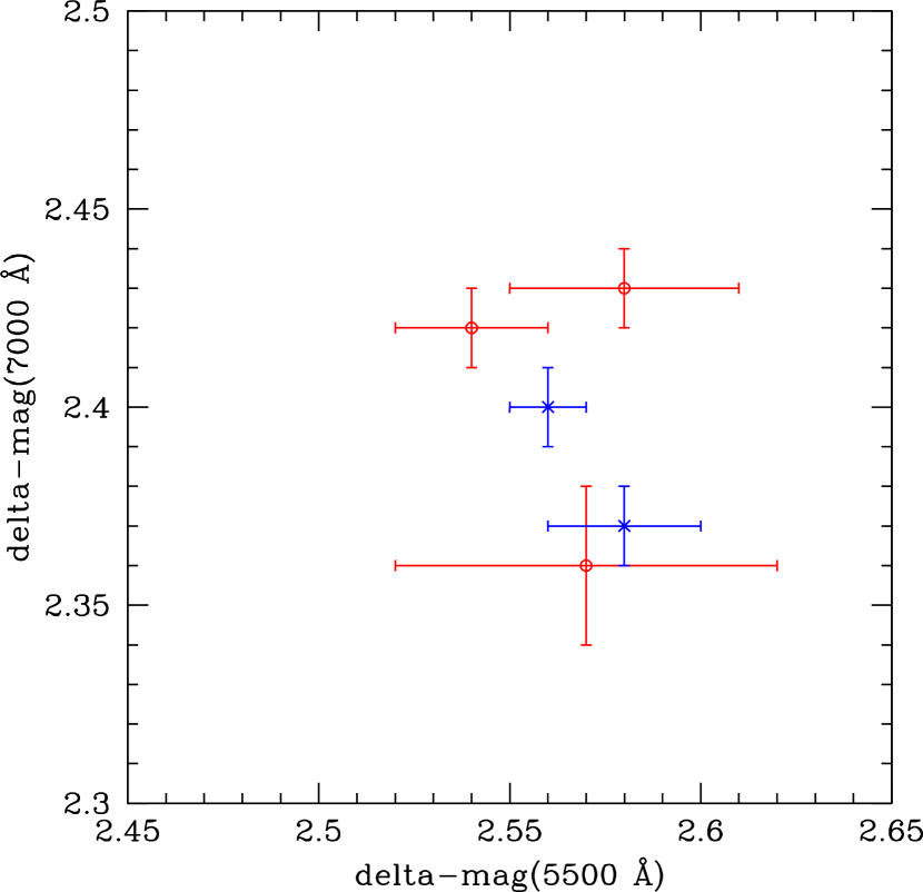
Figure 7: The magnitude difference results for $\phi$ Her from the NPOI data. The red circles show the 1997-1999 results, and the blue x’s the 2004 and 2005 results. Data for this figure are from Table 4.

Figure 10: The predicted radial velocity of the secondary of $\phi$ Her B (solid line) using the orbital elements from Table 3 plotted with the observed radial velocities from Table 5. The radial velocities from Table 5 are averages of the velocities observed on 2004 Jun 10 and 2004 Jul 28.

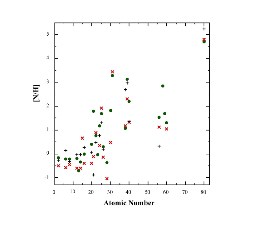
Figure 11: The abundance anomalies [N/H] relative to solar for the HgMn stars HR 7018 (+’s), $\upsilon$ Her (x’s), and $\phi$ Her A (filled circles). They show the general pattern of anomalies for the HgMn stars along with individual scatter.

Table 1: NPOI Observation Log

UT Date	Julian Year	Sids	Baselines	MaxBl	Scans
(1)	(2)	(3)	(4)	(5)	(6)
1997 Apr 19	1997.2972	AC, AE, AW	3	37.5	4
1997 May 08	1997.3492	AC, AE, AW	3	37.5	3
1997 May 30	1997.4094	AC, AE, AW	3	37.5	7
1997 Jun 27	1997.4861	AC, AE, AW	3	37.5	5
1997 Jul 04	1997.5052	AC, AE, AW	3	37.5	6
1998 May 16	1998.3704	AC, AE, AW	3	37.5	18
1998 Jul 04	1998.5046	AC, AE, AW	3	37.5	9
1998 Oct 07	1998.7646	AC, AE, AW	3	37.5	4
1999 Feb 28	1999.1589	E2, E4, AW	3	37.5	4
2004 Apr 30	2004.3280	AC, AE, AW	2	22.2	2
2004 May 01	2004.3307	AC, AE, AW	2	22.2	10
2004 May 03	2004.3362	AC, AE, AW	2	22.2	16
2004 May 04	2004.3389	AC, AE, AW	2	22.2	8
2004 May 05	2004.3417	AC, AE, AW	2	22.2	7
2004 May 06	2004.3444	AC, AE, AW	2	22.2	8
2004 Jul 07	2004.5142	AC, AE, AW, W7, AN	8	66.5	8
2004 Jul 08	2004.5168	AC, AE, AW, W7, AN	8	66.5	8
2004 Jul 09	2004.5197	AC, AE, AW, W7, AN	8	66.5	8
2004 Jul 21	2004.5525	AC, AE, AW	2	22.2	1
2004 Jul 23	2004.5580	AC, AE, AW	2	22.2	13
2004 Jul 30	2004.5771	AC, AE, AW	2	22.2	14
2004 Jul 31	2004.5800	AC, AE, AW	2	22.2	7
2005 May 24	2005.3929	AC, AE, AW, AN, E06	6	53.2	3
2005 Jun 09	2005.4368	AC, AE, AW, AN, E06	6	53.2	4
2005 Jun 16	2005.4561	AC, AE, AW, AN, E06	6	53.2	1

Note. — Col. (1): UT date of NPOI observation. Col. (2): Julian Year at 0700 UT (local midnight). Col. (3): Siderostats used. See Armstrong et al. (1998) for siderostat definitions and locations. Col. (4): Number of baselines. Col. (5) Maximum baseline length (m). Col. (6): Number of interferometric scans obtained.

Table 2: Astrometric Solutions for $\phi$ Her

UT	Julian	$\rho$	$\theta$	$\sigma_{maj}$	$\sigma_{min}$	$\phi$	Cρ	Cθ	(O$-$C)ρ	(O$-$C)θ
Date	Year	(mas)	(deg)	(mas)	(mas)	(deg)	(mas)	(deg)	(mas)	(deg)
(1)	(2)	(3)	(4)	(5)	(6)	(7)	(8)	(9)	(10)	11
Apr 19	1997.2972	37.51	223.59	1.00	0.28	181.0	37.59	223.19	$-$0.08	+0.40
May 08	1997.3492	34.63	231.01	0.69	0.31	163.0	34.49	231.20	+0.14	$-$0.19
May 30	1997.4094	30.50	242.80	0.81	0.28	172.0	30.41	242.65	+0.09	+0.15
Jun 27	1997.4861	24.73	263.16	0.81	0.28	175.6	24.56	263.12	+0.17	+0.04
Jul 04	1997.5052	23.09	269.66	0.89	0.30	141.7	23.04	269.90	+0.05	$-$0.24
May 16	1998.3704	48.54	176.96	0.84	0.27	165.4	48.64	176.80	$-$0.10	+0.16
Jul 04	1998.5046	48.51	188.19	0.95	0.27	171.9	48.45	188.11	+0.06	+0.08
Oct 07	1998.7646	41.40	212.85	1.04	0.34	118.7	41.52	213.13	$-$0.12	$-$0.28
Feb 28	1999.1589	15.79	330.10	1.08	0.28	15.7	15.98	330.84	$-$0.19	$-$0.74
Apr 30	2004.3280	44.16	156.39	0.92	0.44	169.8	43.84	155.99	+0.32	+0.40
May 01	2004.3307	43.77	156.12	0.84	0.46	160.8	43.93	156.27	$-$0.16	$-$0.15
May 03	2004.3362	44.11	156.74	0.87	0.45	160.2	44.13	156.84	$-$0.02	$-$0.10
May 04	2004.3389	44.19	157.19	0.84	0.47	155.0	44.22	157.11	$-$0.03	+0.08
May 05	2004.3417	44.28	157.45	0.83	0.46	159.4	44.31	157.40	$-$0.03	+0.05
May 06	2004.3444	44.31	157.65	0.83	0.46	159.4	44.41	157.67	$-$0.10	$-$0.02
Jul 07	2004.5142	48.31	173.28	0.49	0.19	99.3	48.26	173.32	+0.05	$-$0.04
Jul 08	2004.5168	48.36	173.64	0.42	0.22	104.0	48.29	173.55	+0.07	+0.09
Jul 09	2004.5197	48.39	173.82	0.33	0.32	127.3	48.33	173.79	+0.06	+0.03
Jul 21	2004.5525	49.56	175.39	1.01	0.45	139.7	48.63	176.58	+0.93	$-$1.19
Jul 23	2004.5580	48.72	177.01	0.98	0.41	152.4	48.67	177.05	+0.05	$-$0.04
Jul 30	2004.5771	48.87	178.74	0.96	0.43	149.5	48.77	178.66	+0.10	+0.08
Jul 31	2004.5800	49.22	178.79	1.06	0.42	132.5	48.78	178.90	+0.44	$-$0.11
May 24	2005.3929	15.17	11.44	0.49	0.25	7.0	15.45	12.34	$-$0.28	$-$0.90
Jun 09	2005.4368	17.16	46.12	0.52	0.25	174.0	16.99	46.31	+0.17	$-$0.19
Jun 16	2005.4561	18.07	59.39	0.53	0.24	2.6	18.11	58.88	$-$0.04	+0.51

Note. — Col. (1): UT month and day of NPOI observation Col. (2): Julian Year of NPOI observation. Col. (3): Fitted binary separation. Col. (4): Fitted binary position angle. Col. (5): Semimajor axis of error ellipse. Col. (6): Semiminor axis of error ellipse. Col. (7): Position angle of error ellipse. Col. (8): Calculated binary separation. Col. (9): Calculated binary position angle Col. (10): O$-$C value for binary separation. Col. (11): O$-$C value for binary position angle.

Table 3: Orbital Elements and Stellar Parameters

Data	Value
a (mas)	32.1 $\pm$ 0.2
i (deg)	12.1 $\pm$ 2.9
$\Omega$ (deg)	9.1 $\pm$ 2.5
e	0.522 $\pm$ 0.004
$\omega$ (deg)	351.9 $\pm$ 2.7
T0 (JD)	2450121.8 $\pm$ 1.0
P (days)	564.69 $\pm$ 0.13
M${}_{1}+$M2 (M⊙)	4.7 $\pm$ 0.6
$\gamma$ (km sec${}^{-1})$	$-$16.66 $\pm$ 0.05
K1 (km sec${}^{-1})$	2.5
K2 (km sec${}^{-1})$	8.1
$\chi_{\nu}^{2}$	0.8
DA (mas)	0.4
DB (mas)	0.2

Note. — See §3.1 for a discussion of the methods used to obtain these results. The stellar diameters (D_A,B) were fixed as discussed in that section.

Table 4: Magnitude Difference Results

Year	$\Delta$mag(5500Å)	$\Delta$mag(7000Å)	Number of Epochs
1997	2.54 $\pm$ 0.02	2.42 $\pm$ 0.01	5
1998	2.58 $\pm$ 0.03	2.43 $\pm$ 0.01	3
1999	2.57 $\pm$ 0.05	2.36 $\pm$ 0.02	1
2004	2.56 $\pm$ 0.01	2.40 $\pm$ 0.01	14
2005	2.58 $\pm$ 0.02	2.37 $\pm$ 0.01	3
1997$-$2005	2.57 $\pm$ 0.05	2.39 $\pm$ 0.05	26

Note. — The data for the individual years is plotted in Fig. 7. See §3.1 for an explanation of the net result shown for the years 1997$-$2005.

Table 5: The Radial Velocities of $\phi$ Her B

Central	UT Date	Epoch	Ident.	Laboratory	Wλ	Line Depth	Line Width		RV (km sec-1)
${\lambda}$ (Å)			Wavelength (Å)	(Å)	(mÅ)		(Å)	Observed	Pred.	Diff.
4864	2004 Jun 10	3166.7581	Ti II(82)	4805.104	13	0.011	1.3	-17.6	-13.8	-3.8
			Fe II(42)	4923.930	23	0.020	1.3	-11.8	-13.8	2.0
			Ba II(1)	4934.086	11	0.009	1.3	-17.3	-13.8	-3.5
5140	2004 Jul 28	3214.7204	Mg I(2)	5167.322	40	0.032	1.4	-8.1	-13.4	5.3
			Mg I(2)	5183.604	32	0.026	1.4	-10.4	-13.4	3.0
5278	2005 Jun 24	3575.7405	Fe II(J)	5279.03	36	0.026	1.5	-26.0	-19.7	-6.3

Table 6: Microturbulence Determinations from Fe II Lines

	Number	$\xi_{1}$		$\xi_{2}$
Species	of Lines	(km s-1)	log N/NT	(km s-1)	log N/NT	gf values
Fe II	56	0.3	-4.33$\pm$0.19	0.5	-4.34$\pm$0.19	MF+N4
	182	0.3	-4.34$\pm$0.17	0.6	-4.36$\pm$0.17	MF+N4+KX
	adopted	0.4

Note. — gf value references: MF = Fuhr et al. (1988), KX = Kurucz & Bell(1995), N4 = Fuhr & Wiese (2005). For $\xi_{1}$ and $\xi_{2}$ the abundances are found so that there is no trend of values for lines of different equivalent widths and have minimum scatter, respectively.

Table 7: Abundances of $\phi$ Her Including New Lines

Mult.	$\lambda$(Å)	log gf	Ref.	Wλ(mÅ)	log N/NT
C II			log C/NT = -3.71$\pm$0.20
O I			log O/NT = -3.37$\pm$0.07
12	5329.11	-1.24	WF	8	-3.38
	5329.68	-1.02	WF	13	-3.40
	5330.74	-0.87	WF	18	-3.26
Mg I			log Mg/NT = -4.49$\pm$0.15
2	5167.32	-1.03	WS	11	-4.54
	5172.68	-0.38	WS	34	-4.53
	5183.60	-0.16	WS	35	-4.71
Mg II			log Mg/NT = -4.76$\pm$0.03
Al II			log Al/NT = -6.28
Si II			log Si/NT = -4.83$\pm$0.17
S II			log S/NT = -4.72$\pm$0.21
1	4991.97	-0.25	KX	8	-4.54
7	4925.34	-0.47	WS	5	-4.59
	5009.56	-0.09	WM	8	-4.65
	5032.47	+0.18	WS	9	-4.83
9	4815.55	+0.18	WM	8	-5.02
15	5014.04	+0.03	WM	8	-4.56
38	5320.73	+0.46	WS	6	-4.66
	5345.72	+0.28	WS	6	-4.43
39	5212.62	+0.24	WS	5	-4.57
Ca I			log Ca/NT = -5.14
Ca II			log Ca/NT = -5.51$\pm$0.11
2	8498.02	-1.31	WS	109	-5.37
	8542.09	-0.36	WS	179	-5.46
	8662.14	-0.62	WS	136	-5.67
Sc II			log Sc/NT = -7.33$\pm$0.14
23	5031.02	-0.32	LD	33	-7.37
Ti II			log Ti/NT = -6.21$\pm$0.21
7	5154.07	-1.92	MF	15	-6.10
	5188.68	-1.21	MF	43	-5.98
13	5010.21	-1.34	KX	9	-6.14
17	4798.52	-2.43	MF	5	-6.44
69	5336.78	-1.70	MF	20	-6.15
70	5226.54	-1.30	MF	41	-5.95
	5262.13	-2.11	KX	11	-6.10
71	5013.68	-1.94	KX	8	-6.40
82	4805.09	-1.10	MF	31	-6.17
86	5129.15	-1.39	MF	25	-6.15
	5185.91	-1.35	MF	24	-6.21
103	5211.54	-1.36	KX	10	-6.35
	5268.62	-1.62	MF	7	-6.28
113	5072.28	-0.75	MF	16	-6.42
114	4874.01	-0.79	MF	15	-6.44
V II			log V/NT = -8.07
Cr I			log Cr/NT = -5.12$\pm$0.18
7	5204.51	-0.21	MF	8	-5.04
	5206.03	+0.02	MF	11	-5.14
	5208.42	+0.16	MF	16	-5.05
Cr II			log Cr/NT = -5.25$\pm$0.19
23	5246.75	-2.45	MF	24	-5.15
	5249.40	-2.43	KX	21	-5.24
	5318.41	-3.13	KX	7	-5.15
24	5210.87	-2.94	KX	14	-5.00
	523.250	-2.09	KX	27	-5.20
	5305.84	-2.36	KX	36	-4.82
30	4812.34	-1.80	MF	33	-5.48
	4836.22	-2.25	MF	36	-4.93
	4848.24	-1.14	MF	62	-5.22
	4856.19	-2.26	MF	16	-5.54
	4884.60	-2.08	MF	30	-5.31
43	5232.50	-2.09	KX	28	-5.20
	5237.33	-1.16	MF	62	-5.07
	5274.96	-1.29	KX	56	-5.15
	5279.88	-2.10	MF	36	-4.94
	5280.05	-2.01	KX	19	-5.57
	5308.41	-1.81	MF	35	-5.28
	5310.69	-2.28	MF	23	-5.15
	5313.56	-1.65	MF	46	-5.09
	5334.87	-1.56	KX	45	-5.22
190	4901.62	-0.83	KX	21	-5.45
	4912.46	-0.95	KX	18	-5.45
Mn I			log Mn/NT = -4.91$\pm$0.19
16	4823.52	+0.14	MF	13	-4.88
Mn II			log Mn/NT = -5.01$\pm$0.21
I	4806.82	-1.56	KX	31	-5.04
	4811.62	-2.34	KX	6	-5.25
	4830.06	-1.85	KX	13	-4.98
	4839.74	-1.86	KX	11	-5.09
	4842.33	-2.01	KX	12	-4.85
	4847.60	-1.81	KX	17	-5.23
	5177.65	-1.77	KX	23	-4.75
	5251.82	-1.83	KX	9	-4.76
	5295.40	-0.66	KX	42	-4.69
	5302.44	-1.00	KX	58	-4.57
	6609.26	-2.05	KX	4	-4.94
	6682.38	-3.11	KX	6	-5.12
Fe I			log Fe/NT = -4.14 $\pm$0.20
15	5328.05	-1.47	N4	10	-3.82
289	4871.31	-0.36	N4	9	-3.94
	4872.13	-0.57	N4	6	-3.91
	4891.49	-0.11	N4	8	-4.28
	4957.30	-0.41	N4	9	-3.89
	4957.60	0.23	N4	21	-4.07
383	5232.95	-0.06	N4	20	-3.75
553	5324.18	-0.10	N4	5	-4.33
638	5014.94	-0.30	N4	5	-3.72
984	5005.71	-0.18	KX	7	-3.78
Fe II			log Fe/NT = -4.34$\pm$0.18
31	4893.83	-4.27	N4	3	-4.52
198	6416.92	-2.88	N4	20	-4.25
J	4826.68	-0.44	KX	5	-4.47
	4883.28	-0.64	KX	5	-4.31
	4908.15	-0.30	KX	8	-4.36
	4913.29	+0.01	KX	13	-4.40
	4948.10	-0.32	KX	6	-4.46
	4948.79	-0.01	KX	10	-4.52
	4951.58	+0.18	KX	15	-4.45
	4953.98	-2.76	KX	6	-4.25
	4958.82	-0.65	KX	3	-4.43
	4977.03	+0.04	KX	12	-4.42
	4984.49	+0.01	KX	16	-4.23
	4990.50	+0.18	KX	16	-4.41
	4991.44	-0.57	KX	7	-4.17
	4993.35	-3.65	MF	16	-4.23
	5001.95	+0.90	KX	44	-4.18
	5004.19	+0.50	KX	24	-4.43
	5006.84	-0.43	KX	10	-4.09
	5007.45	-0.37	KX	9	-4.22
	5007.74	-0.20	KX	10	-4.34
	5009.02	-0.42	KX	6	-4.40
	5015.76	-0.05	KX	22	-3.94
	5018.44	-1.22	MF	95	-4.25
	5019.46	-2.70	KX	12	-3.97
	5021.59	-0.30	KX	10	-4.24
	5022.79	-0.02	KX	14	-4.33
	5026.80	-0.22	KX	10	-4.33
	5030.63	+0.40	KX	21	-4.43
	5031.90	-0.78	KX	3	-4.33
	5032.71	+0.11	KX	14	-4.41
	5035.70	+0.61	KX	36	-4.13
	5045.11	-0.13	KX	9	-4.48
	5060.26	-0.52	KX	8	-4.07
	5061.72	+0.22	KX	16	-4.44
	5067.89	-0.20	KX	5	-4.66
	5070.90	+0.24	KX	16	-4.45
	5075.76	+0.28	KX	11	-4.68
	5076.61	-0.71	KX	7	-4.00
	5082.23	-0.10	KX	6	-4.64
	5087.30	-0.49	KX	3	-4.58
	5093.57	+0.11	KX	18	-4.23
	5106.11	-0.28	KX	9	-4.29
	5117.03	-0.13	KX	8	-4.46
	5119.34	-0.56	KX	4	-4.38
	5120.35	-4.21	KX	5	-4.30
	5127.86	-2.54	KX	10	-4.23
	5144.35	+0.28	KX	12	-4.60
	5145.77	-0.40	KX	12	-3.96
	5149.46	+0.40	KX	18	-4.45
	5150.49	-0.12	KX	7	-4.51
	5160.84	-2.64	KX	10	-4.13
	5166.55	-0.03	KX	11	-4.35
	5169.03	-0.87	MF	104	-4.27
	5170.77	-0.36	KX	8	-4.22
	5177.02	-0.18	KX	10	-4.29
	5180.31	+0.04	KX	11	-4.46
	5186.87	-0.30	KX	4	-4.60
	5194.89	-0.15	KX	13	-4.10
	5199.12	+0.10	KX	13	-4.44
	5200.80	-0.37	KX	6	-4.39
	5203.64	-0.05	KX	8	-4.54
	5214.00	-0.22	KX	15	-3.95
	5214.05	-0.90	KX	5	-3.90
	5215.34	-0.10	KX	16	-4.06
	5215.83	-0.23	KX	17	-3.92
	5216.85	+0.81	KX	30	-4.39
	5218.84	-0.20	KX	7	-4.48
	5222.36	-0.33	KX	6	-4.39
	5223.23	-0.41	KX	10	-4.07
	5223.80	-0.59	KX	6	-4.20
	5224.40	-0.57	KX	5	-4.23
	5227.48	+0.85	N4	44	-4.02
	5231.91	-0.64	KX	5	-4.15
	5234.62	-2.05	MF	62	-4.14
	5237.95	+0.14	KX	16	-4.28
	5245.46	-0.51	KX	5	-4.34
	5247.95	+0.55	N4	21	-4.44
	5251.23	0.42	N4	24	-4.19
	5253.64	-0.09	KX	12	-4.22
	5254.41	-0.77	KX	6	-3.96
	5254.93	-3.23	KX	21	-4.25
	5257.12	+0.03	KX	13	-4.25
	5260.26	+1.07	KX	40	-4.37
	5264.18	+0.30	N4	24	-4.08
	5264.81	-3.19	MF	29	-4.04
	5272.40	-2.03	MF	19	-4.14
	5276.00	-1.94	MF	6	-4.30
	5278.21	-1.56	KX	5	-4.24
	5278.94	-2.41	KX	8	-4.32
	5291.67	+0.58	KX	21	-4.49
	5303.39	-1.61	KX	4	-4.30
	5306.18	+0.04	N4	12	-4.31
	5315.08	-0.38	KX	5	-4.34
	5315.56	-1.46	KX	6	-4.28
	5316.23	+0.34	N4	26	-4.10
	5316.78	-2.78	N4	25	-4.58
	5318.05	-0.14	KX	7	-4.46
	5318.75	-0.57	KX	4	-4.34
	5339.59	0.54	KX	23	-4.36
	5347.18	-0.28	KX	6	-4.33
Fe III			log Fe/NT = -4.32
Ni II			log Ni/NT = -6.14$\pm$0.14
Zn I			log Zn/NT = -5.66$\pm$0.18
2	4810.53	-0.14	KX	18	-5.53
Zn II			log Zn/NT = -5.56
3	4911.18	+0.54	WM	18	-5.56
Ga II			log Ga/NT = -5.87$\pm$0.10
Sr II			log Sr/NT = -7.99$\pm$0.08
Y II			log Y/NT = -6.65$\pm$0.17
20	4982.13	-1.29	HL	20	-6.58
	5119.11	-1.36	HL	18	-6.62
	5200.40	-0.57	HL	40	-6.60
	5205.72	-0.34	HL	52	-6.27
	5289.82	-1.85	HL	9	-6.55
22	4823.30	-1.11	HL	29	-6.49
22	4854.86	-0.38	HL	36	-6.97
	4883.68	0.07	HL	58	-6.39
28	5196.42	-0.88	KX	17	-6.73
38	6613.73	-1.11	HL	12	-6.70
Zr II			log Zr/NT = -7.24$\pm$0.20
Ba II			log Ba/NT = -8.36
1	4934.08	0.00	WM	17	-8.36
Ce II			log Ce/NT = -7.61
Hg I			log Hg/NT = -6.14
Hg II			log Hg/NT = -6.19

Note. — gf value references (including those for older lines): BG = Biemont et al. (1989) for V II; Biemont et al. (1981) for Zr II, DW = Dworetsky (1980), GB = Grevesse et al. (1981), HL = Hannaford et al. (1982), KX = Kurucz & Bell (1995), LA = Lanz & Artru (1985), LD = Lawler & Dakin (1989), MF = Fuhr et al. (1988) and Martin et al. (1988), MC = Magazzu & Cowley (1986), N4 = Fuhr & Wiese (2005), WF = Wiese, Fuhr & Deters (1996),WM = Wiese & Martin (1980), WS = Wiese, Smith & Glennon (1966) and Wiese, Smith & Miles (1969) The adopted abundance from Hg II $\lambda$3984 is from Woolf & Lambert (1999b). The multiplet numbers are from Moore (1945) except that I indicates Mn II lines from Iglesias & Velasco (1964) and J indicates Fe II lines from Johansson (1978 ).

Table 8: Comparison of Derived and Solar Abundances (log N/H)

	$\phi$ Her A	$\phi$ Her A	Number
Species	Adelman et al. (2001)	This Paper	of Lines	Sun
He I	-1.21$\pm$0.05	-1.17$\pm$0.05	7	-1.01
C II	-3.76$\pm$0.25	-3.68$\pm$0.20	3	-3.45
O I	-3.17$\pm$0.49	-3.34$\pm$0.07	4	-3.13
Mg I	-4.54$\pm$0.41	-4.46$\pm$0.15	5	-4.42
Mg II	-4.78$\pm$0.03	-4.75$\pm$0.03	5	-4.42
Al II	-6.27	-6.25	1	-5.53
Si II	-4.95$\pm$0.22	-4.80$\pm$0.17	11	-4.45
S II	-4.41$\pm$0.25	-4.69$\pm$0.21	22	-4.67
Ca I	-5.14	-5.11	1	-5.64
Ca II	-5.56	-5.48$\pm$0.11	4	-5.64
Sc II	-7.39$\pm$0.14	-7.03$\pm$0.14	12	-8.83
Ti II	-6.32$\pm$0.29	-6.21$\pm$0.21	66	-6.98
V II	-8.11	-8.04	1	-8.00
Cr I	-5.16$\pm$0.28	-5.09$\pm$0.18	7	-6.33
Cr II	-5.39$\pm$0.25	-5.22$\pm$0.19	64	-6.33
Mn I	-4.86$\pm$0.22	-4.88$\pm$0.19	18	-6.61
Mn II	-4.95$\pm$0.29	-4.98$\pm$0.21	71	-6.61
Fe I	-4.19$\pm$0.22	-4.11$\pm$0.20	70	-4.50
Fe II	-4.45$\pm$0.20	-4.31$\pm$0.18	182	-4.50
Fe III	-4.35	-4.29	1	-4.50
Ni II	-6.30$\pm$0.30	-6.11$\pm$0.14	4	-5.75
Zn I	-5.80	-5.63$\pm$0.18	2	-7.40
Zn II	-5.61	-5.53	1	-7.40
Ga II	-5.85$\pm$0.18	-5.84$\pm$0.10	2	-9.12
Sr II	-8.05$\pm$0.14	-7.96$\pm$0.08	3	-9.03
Y II	-6.79$\pm$0.23	-6.62$\pm$0.17	21	-9.76
Zr II	-7.30$\pm$0.25	-7.21$\pm$0.20	33	-9.40
Ba II	-7.69	-8.33	1	-9.87
Ce II	-7.63	-7.58	1	-10.42
Pr	….	-9.60	…	-11.29
Nd	….	-9.30	…	-10.59
Hg I	-6.15	-6.11	1	-10.83
Hg II	-6.41	-6.16	1	-10.83

Note. — The Hg II value adopted for this study is that of Woolf & Lambert (1999b), the Nd and Pr abundances are from Dolk et al. (2002), and the solar values are from Grevesse, Noels & Sauval (1996). When more than one line is detected the error is the standard deviation of the mean. No error is quoted when only one line is present.

Table 9: Stellar Parameters of $\phi$ Her A and B

Component	Teff	log (g)	vsin(i)
	(K)	log(cm sec-2)	(km sec-1)
A	11525 $\pm$ 150	4.05 $\pm$ 0.15	8.0 $\pm$ 1.0
B	8000 $\pm$ 150	4.30 $\pm$ 0.15	50.0 $\pm$ 3.0

References

- Adelman & Pyper (1983) Adelman, S. J., & Pyper, D. M., 1983, A&A, 118, 313
- Adelman, Gulliver & Rayle (2001) Adelman, S. J., Gulliver, A. F., & Rayle, K. E. 2001, A&A, 367, 597
- Adelman et al. (2004a) Adelman S. J., Gulliver, A. F., Smalley, B., Pazder, J. S., Boyd, L. J., & Epand, D. 2004, in The A-Star Puzzle, ed. J. Zverko, J. Ziznovsky. S. J. Adelman, and W. W. Weiss (Cambridge: Cambridge University Press), 911
- Adelman et al. (2004b) Adelman, S. J., Proffitt, C. R., Wahlgren, G. M., Leckrone, D. S., Dolk, L. 2004, ApJS, 155, 179
- Adelman et al. (2006) Adelman S. J., Caliskan H., Gulliver A. F., & Teker, A. 2006, A&A, 447, 685
- Adelman et al. (2007) Adelman, S. J., Gulliver, A. F., Smalley, B., Pazder, J. S., Boyd, L. J., Epand, D. & Younger, T. 2007, in The Future of Photometric, Spectrophotometric, and Polarimetric Standardization, ed. C. Sterken (San Francisco, ASP), ASPC, in press
- Aikman (1976) Aikman, G. C. L. 1976, Publications of the Dominion Astrophysical Observatory Victoria, 14, 379
- Andersen (1991) Andersen, J. 1991, A&A Rev., 3, 91
- Armstrong et al. (1998) Armstrong, J. T., et al. 1998, ApJ, 496, 550
- Babcock (1971) Babcock, H.W. 1971, Carnegie Institution Yearbook, 70, 404
- Batten et al. (1989) Batten, A. H., Fletcher, J. M., & MacCarthy, D. G. 1989, Publications of the Dominion Astrophysical Observatory Victoria, 17, 1
- Benson et al. (1997) Benson, J. A., et al. 1997, AJ, 114, 1221
- Benson et al. (2003) Benson, J. A., Hummel, C. A., & Mozurkewich, D. 2003, Proc. SPIE, 4838, 358
- Biemont et al. (1981) Biemont E., Grevesse N., Hannaford P., & Lowe R. M., 1981, ApJ, 248, 867
- Biemont et al. (1989) Biemont E., Grevesse N., Faires L. M., Marsden G., Lawler J. E., & Whaling W., 1989, A&A, 209, 391
- Blackwell, Shallis & Simmons (1982) Blackwell D. E., Shallis M. J., & Simmons G. J., 1982, MNRAS, 199, 33
- Cannon & Pickering (1921) Cannon, A. J., & Pickering, E. C. 1921, Annals of Harvard College Observatory, 96, 1
- Cornwell et al. (1999) Cornwell, T., Braun, R., & Briggs, D. S. 1999, ASP Conf. Ser. Vol. 180: Synthesis Imaging in Radio Astronomy II, ed. G. B. Taylor, C. L. Carilli & R. A. Perley (San Francisco: ASP)
- Cox (2000) Cox, A. N. 2000, Allen’s Astrophysical Quantities, ed. A. N. Cox (4th Edition: New York: AIP Press)
- Dolk et al. (2002) Dolk, L., Wahlgren, G. M., Lundberg, H., Li, Z. S., Litzén, U., Ivarsson, S., Ilyin, I., & Hubrig, S. 2002, A&A, 385, 111
- Dworetsky (1980) Dworetsky M. M., 1980, A&A, 84, 350
- Fuhr (2005) Fuhr J. R., & Wiese W. L., 2005, J. Phys. Chem. Ref. Data, in press
- Fuhr, Martin & Wiese (1988) Fuhr J. R., Martin G. A., & Wiese W. L., 1988, J. Phys. Chem. Ref. Data, 17, Suppl. 4
- Gigas (1986) Gigas, D. 1986, A&A, 165, 170
- Grevesse, Biemont, Hannaford & Lowe (1981) Grevesse N., Biemont E., Hannaford P., & Lowe R. M., 1981, in Upper Main Sequence Stars, 23rd Liege Astrophys. Colloq. (Liege: Universite de Liege), 211
- Grevesse, Noels & Sauval (1996) Grevesse N., Noels A., & Sauval A. 1996, ASPC, 99, 117
- Gulliver & Hill (2002) Gulliver A. F., Hill G. 2002, In: Astronomical Data Analysis Software and System XI, in ASP Conf. Ser. Vol. 281, ed. D. A. Bohlender, D. Durand, & T. H. Handley (San Francisco, ASP), 351
- Hannaford, Lowe, Grevesse & Biemont (1982) Hannaford P., Lowe R. M., Grevesse N., & Biemont E., 1982, ApJ, 261, 736
- Hartkopf, Mason & Worley (2001) Hartkopf, W.I., Mason, B.D., & Worley, C.E. 2001, Sixth Catalog of Orbits of Visual Binary Stars (Washington, D.C.: U.S. Naval Observatory) http://www.ad.usno.navy.mil/wds/orb6/orb6.html
- Hayes & Latham (1975) Hayes, D. S., & Latham, D. W. 1975, ApJ, 197, 593
- Heintz (1978) Heintz, W. D. 1978, Double Stars, Geophysics and Astrophysics Monographs Vol. 15 (D. Reidel: Dordrecht)
- Hill, Fisher, & Poeckert (1982) Hill G., Fisher, W. A., & Poeckert R., 1982, Publ. Dom. Astrophys. Obs. Victoria 16, 27
- Högbom (1974) Högbom, J. A. 1974, A&AS, 15, 417
- Hoffleit & Jaschek (1982) Hoffleit, D., & Jaschek, C. 1982, The Bright Star Catalogue (4th Edition: New Haven: Yale University Observatory)
- Hubeny, Lanz & Jeffrey (1994) Hubeny, I., Lanz T., & Jeffrey C. S., 1994, Daresbury Lab. New. Anal. Astron. Spectra. No 20, 20
- Hummel et al. (1998) Hummel, C. A., Mozurkewich, D., Armstrong, J. T., Hajian, A. R., Elias, N. M., & Hutter, D. J. 1998, AJ, 116, 2536
- Hummel et al. (2003) Hummel, C. A., et al. 2003, AJ, 125, 2630
- Hutter et al. (2005) Hutter, D. J., et al. 2005, Proc. SPIE, in press
- Iglesias & Velasco (1964) Iglesias L., & Velasco R. 1964, Publ. Inst. Opt. Madrid, No. 23
- Jennison (1958) Jennison, R. C. 1958, MNRAS, 118, 276
- Johansson (1978) Johansson S. 1978, Phys. Scripta 18, 217
- Kurucz (1979) Kurucz, R. L. 1979, ApJS, 40, 1
- Kurucz (1993) Kurucz R. L. 1993, ATLAS9 Stellar Atmosphere Programs and 2 km sec-1 grid, Kurucz CD-Rom No. 13, Smithsonian Astrophysical Observatory, Cambridge, MA
- Kurucz & Bell (1995) Kurucz R. L., & Bell B. 1995, Atomic Data for Opacity Calculations, Kurucz CD-Rom No. 23, Smithsonian Astrophysical Observatory, Cambridge, MA
- Kurucz & Avrett (1981) Kurucz R. L., & Avrett E. H. 1981, SAO Special Report No. 391
- Lanz & Artru (1985) Lanz T., & Artru M.-C. 1985, Phys. Scripta, 32, 115
- Lawler & Dakin (1989) Lawler, J. E., & Dakin, J. T. 1989, JOSA B, 6, 1457
- Leckrone et al. (1991) Leckrone, D. S., Wahlgren, G. M., & Johansson, S. G. 1991, ApJ, 377, L37
- Lemke (1989) Lemke, M. 1989, A&A, 225, 125
- Lindegren et al. (1997) Lindegren, L., et al. 1997, A&A, 323, L53
- Magazzu & Cowley (1986) Magazzu A., & Cowley C. R. 1986, ApJ, 134, 562
- Martin, Fuhr & Wiese (1988) Martin G. A., Fuhr J. R., & Wiese W. L. 1988, J. Phys. Chem. Ref. Data 17, Suppl. 3
- Mason et al. (1999) Mason, B. D., et al. 1999, AJ, 117, 1890
- Michaud (1970) Michaud, G. 1970, ApJ, 160, 641
- Moore (1945) Moore C. E. 1945, A Multiplet Table of Astrophysical Interest (Princeton: Princeton University Observatory)
- Morgan (1933) Morgan, W. W. 1933, ApJ, 77, 330
- Morgan & Keenan (1973) Morgan, W. W., & Keenan, P. C. 1973, ARA&A, 11, 29
- Mozurkewich et al. (1991) Mozurkewich, D., et al. 1991, AJ, 101, 2207
- Osawa (1965) Osawa, K. 1965, Annals of the Tokyo Astronomical Observatory, 9, 121
- Pan et al. (1992) Pan, X., et al. 1992, ApJ, 384, 624
- Perryman et al. (1997) Perryman, M. A. C., et al. 1997, A&A, 323, L49
- Preston (1974) Preston, G. W. 1974, ARA&A, 12, 257
- Reader & Corliss (1980) Reader J., & Corliss C. H. 1980, NSRDS-NBS 68, Part 1, US Government Printing Office, Washington, DC
- Roby et al. (1999) Roby, S. R., Leckrone, D. S., & Adelman, S. J. 1999, ApJ, 524, 974
- Shepherd (1997) Shepherd, M. C. 1997, in ASP Conf. Ser. 125, Astronomical Data Analysis Software and Systems VI, ed. G. Hunt & H. E. Payne (San Francisco: ASP), 77
- Shepherd, Pearson & Taylor (1994) Shepherd, M. C., Pearson, T. J., & Taylor, G. B. 1994, BAAS, 26, 987
- Smalley & Dworetsky (1995) Smalley, B & Dworetsky, M. M. 1995, A&A, 293, 446
- Stickland & Dworetsky (1980) Stickland, D. J., & Dworetsky, M. M. 1980, MNRAS, 191, 33P
- Thompson, Moran & Swenson (1999) Thompson, A. R., Moran, J. M. & Swenson, G. W. 2001, Interferometry and Synthesis in Radio Astronomy (2nd. Edition: New York; John Wiley & Sons), 69
- White & Feierman (1987) White, N. M., & Feierman, B. H. 1987, AJ, 94, 751
- Wiese, Fuhr & Deters (1996) Wiese W. F., Fuhr J. R., & Deters T. M. 1996, J. Phys. Chem. Ref. Data, Monograph 6
- Wiese & Martin (1980) Wiese W. L., & Martin G. A. 1980, NSRDS-NBS 68, Part 2, US Government Printing Office, Washington, DC
- Wiese, Smith & Glennon (1966) Wiese W. L., Smith M. W., & Glennon B. M., 1966, NSRDS-NBS 4, US Government Printing Office, Washington, DC
- Wiese, Smith & Miles (1969) Wiese W. L., Smith M. W., & Miles B. M., 1969, NSRDS-NBS 22, US Government Printing Office, Washington, DC
- Wittkowski et al. (2001) Wittkowski, M., Hummel, C. A., Johnston, K. J., Mozurkewich, D., Hajian, A. R., & White, N. M. 2001, A&A, 377, 981
- Woolf & Lambert (1999a) Woolf V. M., & Lambert D. L., 1999a, ApJ, 520, L55
- Woolf & Lambert (1999b) Woolf V. M., & Lambert D. L., 1999b, ApJ, 521, 414
- Woolf & Woolf (1976) Woolf, S. C. & Woolf, R. J. 1976, in Physics of Ap Stars, Proceedings of the IAU Colloquium held at the Vienna Observatory, eds. W. W. Weiss, H. Jenkner & H. J. Wood (Vienna: Universitätssternwarte Wien)
- Zavala et al. (2004) Zavala, R. T., et al. 2004, BAAS 36(5), No. 107.15