Interplanetary and interstellar plasma turbulence
Abstract
Theoretical approaches to low-frequency magnetized turbulence in collisionless and weakly collisional astrophysical plasmas are reviewed. The proper starting point for an analytical description of these plasmas is kinetic theory, not fluid equations. The anisotropy of the turbulence is used to systematically derive a series of reduced analytical models. Above the ion gyroscale, it is shown rigourously that the Alfvén waves decouple from the electron-density and magnetic-field-strength fluctuations and satisfy the Reduced MHD equations. The density and field-strength fluctuations (slow waves and the entropy mode in the fluid limit), determined kinetically, are passively mixed by the Alfvén waves. The resulting hybrid fluid-kinetic description of the low-frequency turbulence is valid independently of collisionality. Below the ion gyroscale, the turbulent cascade is partially converted into a cascade of kinetic Alfvén waves, damped at the electron gyroscale. This cascade is described by a pair of fluid-like equations, which are a reduced version of the Electron MHD. The development of these theoretical models is motivated by observations of the turbulence in the solar wind and interstellar medium. In the latter case, the turbulence is spatially inhomogeneous and the anisotropic Alfvénic turbulence in the presence of a strong mean field may coexist with isotropic MHD turbulence that has no mean field.
1 Introduction
Rapid progress in astronomical instrumentation has made it possible to observe astrophysical plasmas with ever greater spatial resolution. This has allowed astronomers to probe not only the bulk, large-scale motions and fields but also to measure, either directly or via line-of-sight integrated quantities associated with the emission and propagation of light, the small-scale fluctuations of plasma velocity, density, magnetic and electric fields. These turbulent fluctuations existing in a broad range of scales are a common property of astrophysical plasmas. While astrophysical turbulence occurs in a variety of vastly differing conditions, its physical characterization is based on a number of universal features. In most cases, the source of energy is in the form of random stirring or instabilities associated with the scale of the astrophysical object of interest. The energy injected at large scales cascades to much (typically many orders of magnitude) smaller scales to be dissipated into heat. A signature property of the turbulent cascade that connects these vastly disparate scales is power-law spectra of the fluctuating quantities. These have been observed in the solar wind (SW), e.g. [36, 2, 24], the interstellar medium (ISM) [1, 42, 35], galaxy clusters [53, 57], etc. In all of the cited examples, the reported spectra had, or were consistent with, Kolmogorov scaling .
In this paper, we shall concentrate on the SW and ISM and outline both the qualitative understanding that currently exists of the turbulence in these media and a formal mathematical description of this turbulence that must underlie the future analytical and numerical investigations of it. The proper starting point for such a description is the kinetic plasma theory because the turbulent plasmas we are interested in are either collisionless (in the SW, the particle mean free path is comparable to the distance from the Sun to the Earth) or only weakly collisional, meaning that the mean free path exceeds the ion gyroradius (in the ISM, cm, cm).
In many cases, it is plausible to think of plasma turbulence at scales much smaller than the energy-injection scale as an ensemble of interacting MHD waves propagating along a dynamically strong background magnetic field (the mean field) associated with the large scales [32]. Goldreich and Sridhar [20] (henceforth, GS) conjectured that in such a turbulence, (i) all electromagnetic perturbations are strongly anisotropic, so that the characteristic wavenumbers along the field are much smaller than those across it, ; and (ii) the interactions between the Alfvén waves are strong, i.e., the Alfvén time and the nonlinear interaction time are comparable to each other:
| (1) |
where is the typical frequency of perturbations, is the Alfvén speed, and is the velocity fluctuation perpendicular to the mean field. This assumption, known as the critical balance, removed dimensional ambiguity from the MHD turbulence theory and led to the Kolmogorov scaling of the Alfvén-wave energy spectrum, and to the relation (for a historical review, see [50]; in A, we give a brief outline of the GS theory and related scaling arguments for MHD turbulence).
The anisotropy of MHD turbulence is supported by observations of the SW the ISM (see reviews [24, 35]) and by numerical simulations [39, 13, 43, 12]. In what follows, this anisotropy emerges as the key simplifying feature used to derive a reduced version of the plasma kinetic theory that describes low-frequency MHD turbulence. This is done in §2, where our exposition is motivated by the observations of the collisionless SW. We show how the descriptions known as Reduced MHD, Kinetic MHD, Electron MHD and Gyrokinetics fit into a single theoretical framework. In §3, we explain how the same approach works for the turbulence in parts of the ISM and how this type of turbulence differs from the isotropic MHD turbulence, which does not have a mean field. We argue that the latter kind of turbulence may also be present in the ISM and in galaxy clusters.
2 Solar wind and the collisionless MHD turbulence
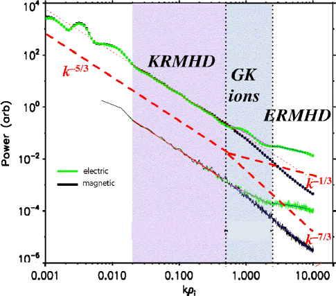
Spectra of electromagnetic fluctuations in the SW extend across a broad range of collisionless scales. Above the ion gyroscale ( km), the spectra of the electric and magnetic field measured by spacecraft at 1 AU from the Sun fit the law and follow each other with remarkable precision (figure 1). Since the electric field is directly related to the plasma velocity (at scales above , it is the drift velocity), this can be interpreted as a signature of Alfvénic turbulence. How do we describe such a turbulence at collisionless scales? Let us first consider scales larger than the ion gyroscale.
Note that the plasma beta is taken to be order unity in what follows, as is appropriate both for the SW and the ISM. It is useful to remember that in this regime, the ion inertial scale is comparable to .
2.1 Kinetic MHD
For , the magnetic field impedes free particle motion across the field lines and the kinetic theory reduces to the so-called Kinetic MHD (KMHD) [34], which has most features of the MHD description, but allows for anisotropic pressure:
| (2) | |||
| (3) | |||
| (4) |
where is mass density, velocity, magnetic field, , and . The pressure tensor is calculated kinetically: and , where the distribution function satisfies
| (5) |
where and . In the above, and are the mass and charge of the particles of species (ions, electrons). The parallel electric field is determined from the quasineutrality condition , where (the number density). Note that and , so (2) and the parallel component of (3) can be derived from (5).
We consider a uniform static equilibrium with a straight mean field in the direction, so and , , , where , , are constant in space and time.
2.2 The ordering
The anisotropy of the turbulence allows us to systematically expand (2)-(5) in . The key step in setting up such an expansion is to estimate the strength of the fluctuations by adopting the critical-balance conjecture (1), but as an ordering assumption rather than a detailed scaling prescription: this means that the wave propagation terms are assumed to be same order as the nonlinear interaction terms (the turbulence is strong). This leads to the following ordering:
| (6) |
where . Two auxiliary ordering assumptions have been made: (i) the perpendicular velocity and magnetic-field fluctuations are Alfvénic (); (ii) the Alfvénic fluctuations are same order as magnetic-field-strength (), density and pressure fluctuations (in the collisional MHD limit, these correspond to the slow waves and the entropy mode). The validity of the latter assumption depends on how the turbulence is stirred. In astrophysical contexts, the large-scale energy input may be assumed to inject comparable power into all types of fluctuations. We also assume that the characteristic frequency of the fluctuations is . The fast waves are, thus, ordered out, because their frequency is .
2.3 Alfvén-wave turbulence: Reduced MHD
The Alfvénic fluctuations are two-dimensionally solenoidal: since [from (2)] and exactly, separating the part of these divergences gives . Therefore, to lowest order, we may write and . Equations for the scalar fields and (the stream and flux functions) are obtained by substituting these expressions into the perpendicular parts of (3) and (4) — of the former the curl is taken to annihilate the pressure term. Keeping only the terms of the lowest order, , we get
| (7) | |||
| (8) |
where and we have taken into account that, to lowest order,
| (9) |
The closed system (7)-(8), known as the Reduced MHD (RMHD), was derived originally from the fluid MHD equations for the studies of stability of fusion plasmas [56, 29]. We have now shown that the Alfvén-wave cascade in a collisionless plasma is described by the RMHD equations (7)-(8) all the way down to the ion gyroscale. The Alfvén waves are decoupled from the other fluctuation modes: density and magnetic-field-strength fluctuations (slow waves and entropy fluctuations in the collisional limit; cf. [21, 37]).
Introducing Elsasser fields , we may rewrite (7)-(8) as follows
| (10) |
Thus, the RMHD, like the MHD, supports wave packets of arbitrary shape and magnitude propagating in one direction at the Alfvén speed : if or , the nonlinear terms vanish and the exact solution for the other Elsasser potential is , where is an arbitrary function. The Alfvén-wave cascade is a result of interactions between counterpropagating wave packets [32].
It is this Alfvénic component of the plasma turbulence to which the GS scaling theory of MHD turbulence (A) applies. In the SW, it is observed via in situ measurements of the fluctuating magnetic and electric fields [2] (see figure 1). The latter directly probe the velocity fluctuations because, to lowest order in , , where is the scalar potential. Clearly, .
2.4 Density and magnetic-field-strength fluctuations: Kinetic Reduced MHD
In order to determine and , we must use the kinetic equation (5).111These quantities cannot be derived from (2) and the parallel part of (4) because (i) (2) has already been used to determine , a quantity; (ii) the parallel part of (4) contains , whose evolution equation, the parallel part of (3), requires , so can only be calculated kinetically. The lowest-order (equilibrium) distribution is taken to be a Maxwellian: , where is the thermal speed of species and is temperature.222The assumption of an isotropic equilibrium was implicit when we adopted an isotropic zeroth-order pressure at the end of §2.1. Strictly speaking, in a collisionless plasma such as the SW, the equilibrium distribution does not have to be Maxwellian or isotropic. The conservation of the first adiabatic invariant, , suggests that temperature anisotropy with respect to the magnetic-field direction () may exist. Such anisotropy gives rise to several high-frequency plasma instabilities [19] and it is plausible to assume that fluctuations associated with them will scatter particles and limit the anisotropy (e.g., [30]). While there is no definitive analytical theory quantifying this idea, it has some support in the SW observations that indicate that the core particle distribution is only moderately anisotropic [40]. We believe, therefore, that assuming a Maxwellian equilibrium is an acceptable simplification. We also take (generalising to is straightforward). Note that in plasmas such as the ISM, where collisions are weak but non-negligible (§3.1), the Maxwellian equilibrium is rigourously justifiable if the ion collision rate is ordered within the expansion [26]. We let , where and apply the ordering (6) to the kinetic equation (5).
The electron kinetic equation can be further simplified by a subsidiary expansion in [48]. To lowest order,
| (11) |
Since , the inhomogeneous solution of this equation is (the electrons are isothermal). The homogeneous solution satisfies , i.e., it is constant along the perturbed field lines and is constant everywhere if the field lines are assumed to be stochastic. Thus, . Substituting this into the ion kinetic equation, we have, to lowest order, ,
| (12) |
Finally, we calculate and . From quasineutrality, , so
| (13) |
To calculate , we first revisit the the perpendicular part of (3). In the lowest order, , it reduces to the perpendicular pressure balance: , whence (this is why the fast waves disappear under our ordering). Now . Using to get , equation (13) to express , and calculating from , we find
| (14) |
where . Note that is not required to solve the equations, but can be calculated from the solution.
Together with (7)-(8), (12)-(14) form a closed system that describes the anisotropic turbulence above the ion gyroscale in a collisionless magnetized plasma. We shall refer to this hybrid fluid-kinetic theory as Kinetic RMHD (KRMHD). The nonlinearity enters in (12) via the derivatives defined in (9) and is due solely to interactions with Alfvén waves. Thus, the cascades of density and magnetic-field-strength fluctuations occur via passive mixing by Alfvén waves, with no energy exchange (cf. [21, 37]).
2.5 Parallel and perpendicular cascades
Let us transform (12) to the Lagrangian frame associated with the velocity field of the Alfvén waves: , where . In this frame, [defined in (9)] becomes . Equation (4) has the Cauchy solution: , where . Then , where is the arc length along the magnetic field line taken at [if , ]. Thus, in the Lagrangian frame associated with the Alfvén waves, (12) is linear. It does not, therefore, support a cascade of and to smaller scales parallel to the perturbed magnetic field, i.e., of these fluctuations does not change with time. In contrast, passive mixing by the Alfvén waves does cause a perpendicular cascade of and — i.e., a cascade in .
Unlike (12), the RMHD equations (7)-(8) in the Lagrangian frame do not reduce to a linear form, so the Alfvén waves should develop small scales both across and along the perturbed magnetic field. The scale-by-scale critical balance (1) conjectured by GS leads to the relation (see A).
Using the linearity of (12) in the Largangian frame, it is straightforward to show that density and field-strength fluctuations are damped. The dispersion relation is
| (15) |
where is the plasma dispersion function and and are the Lagrangian frequency and wave number (). When , all solutions of (15) have damping rates .333For , the weakest-damped solution is . This is the anisotropic limit () of the more general effect known as Barnes, or transit-time, damping [3]. Note that we carried out the expansion in small before taking the high- limit. A more standard approach in the linear theory of plasma waves is to leave arbitrary and take the high- limit first [16]. If no parallel cascade of and develops, the parallel wavenumber of these fluctuations with a given does not grow with , so, for large enough , it is much smaller than the parallel wave number of the Alfvén waves that have the same . This means that the damping rate is small compared to the characteristic rate at which the Alfvén waves cause and to cascade to higher . One is then led to conclude that, despite the kinetic damping, and should have perpendicular cascades extending to the ion gyroscale.
The validity of this conclusion is not quite as obvious as it might appear. Lithwick and Goldreich [37] argued that the dissipation of and at the ion gyroscale would lead these fluctuations to become uncorrelated at the same parallel scales as the Alfvénic fluctuations by which they are mixed, i.e., . The damping rate then becomes comparable to the cascade rate, causing the cascades of density and field-strength fluctuations to be cut off at . In the SW, this would mean that no such fluctuations should be detected above the ion gyroscale. Observational evidence is at odds with this conclusion: the density fluctuations appear to follow a law at [11], as they should if they are passively mixed and not damped (see A). The same is true for the fluctuations of the field strength [6, 23]. It is not clear why Lithwick and Goldreich’s argument fails, but it is, perhaps, useful to point out two potential pitfalls: (i) in order for the dissipation terms, not present in (12)-(14), to act, the density and field-strength fluctuations should reach the ion gyroscale in the first place; (ii) the damping rate of these fluctuations, even if , is never much larger than the cascade rate, so it may be necessary to have a quantitative calculation of the interplay between the kinetic damping, mixing and the dissipation at in order to determine the efficiency of the cascade.
2.6 Gyrokinetics
At , the KMHD description breaks down and the Alfvénic fluctuations are no longer decoupled from the kinetic component of the turbulence. They are mixed with the fluctuations of the density and magnetic-field strength and dissipated via the collisionless damping discussed in §2.5 — the observed flattening of the density-fluctuation spectrum as approaches unity [11] is likely to be due to this energy exchange with the Alfvén waves. The damping leads to ion heating, an astrophysically interesting problem in its own right, e.g., in the theories of coronal heating [14] and accretion discs [45]. The amount of heating suffered by the ions is a nontrivial issue because only part of the turbulent energy is dissipated at . The rest is converted into a cascade of kinetic Alfvén waves (KAW) that extends to the electron gyroscale — a feature observed in the SW [36, 2]. Quantitative theory or numerical modeling of the energy dissipation and conversion processes at can only be done in the fully kinetic framework. However, the anisotropy of the fluctuations leads to a substantial simplification of the full plasma kinetic theory. If the ordering based on the assumptions of anisotropy and critical balance (§2.2) is applied, the plasma kinetics reduce to gyrokinetics (GK) — a low-frequency limit well known in fusion science [10]. A simple derivation of GK based on the ordering of §2.2 is given in [26], along with a detailed GK treatment of the linear collisionless damping at . The GK is a valid approximation at all scales that are of interest in the context of low-frequency astrophysical turbulence, down to the electron gyroscale and below. This broad range of validity and the long experience of GK simulations developed in fusion research make GK an ideal tool for numerical modeling of astrophysical turbulence444A programme of such numerical studies, using the GS2 code [http://gs2.sourceforge.net/], is currently underway (supported by the US DOE Center for Multiscale Plasma Dynamics). and a good starting point for analytical theory.
The RMHD and KRMHD equations (§§2.3,2.4) can be derived from GK by means of two subsidiary expansions: first in , then in .555This means that the , and expansions commute: KRMHD can be arrived at by either of the two routes: full kinetics expansion KMHD expansion expansion isothermal electrons KRMHD [this paper] or full kinetics expansion GK [26] expansion isothermal electrons expansion KRMHD [52]. This and various other limits of the GK description of turbulence in weakly collisional astrophysical plasmas are worked out in [52]. While the regime requires solving the ion GK equation (electrons remain isothermal [52]), the KAW turbulence at is described by another well known fluid model, the Electron MHD (EMHD) [31].
2.7 Kinetic Alfvén waves: Electron Reduced MHD
When , the ions are unmagnetized and have a Boltzmann distribution: , where is the scalar potential. The electrons are magnetized () and can be shown to be isothermal in essentially the same way as in §2.4, where (11) is still valid to lowest order in . Then
| (16) |
The last equality follows from the (perpendicular) pressure balance similarly to the way it was done in §2.4, using (the ordering of §2.2, which eliminates the fast waves, continues to be valid). The EMHD equations now follow from the density and parallel velocity moments of the electron kinetic equation, which is similar in form to (12). The rigourous GK derivation is given in [52]. Here, we adopt a more conventional approach by noting that in the limit , the magnetic field is frozen into the electron fluid and satisfies (4) with replaced by the electron flow velocity [31]:
| (17) |
We set and expand (17) using the ordering of §2.2. To lowest order in the expansion, can be found by taking the ions to be immobile and using Ampère’s law: . In the last term in (17), the next-order compressible part of is calculated via the electron continuity equation: . Finally, using (16) and denoting [see (16)], we find that the parallel and perpendicular components of (17) take the following form
| (18) | |||
| (19) |
where is defined in (9). We shall refer to this system as Electron Reduced MHD (ERMHD) — the anisotropic limit of EMHD.666 Equation (17) with and (the incompressible limit valid if ) is what is normally understood by EMHD. In (18)-(19), is arbitrary, i.e., the electron fluid is not assumed to be exactly incompressible.
ERMHD describes the cascade of kinetic Alfvén waves (KAW), whose linear dispersion relation is with eigenfunctions . To understand the nonlinear cascade, one may follow the spirit of GS theory, assuming anisotropy () and strong interactions [7, 12]. This argument, reviewed at the end of A, leads to a spectrum of magnetic fluctuations (note that for KAW-like fluctuations, ) and to the relation , quantifying the anisotropy. Both of these scalings have been confirmed by numerical simulations of EMHD [7, 12]. Note that the electric-field fluctuations in this regime should have a spectrum because . Measurements of the spectra of and in the SW appear to corroborate these arguments [2] (see figure 1).
The anisotropic KAW cascade is terminated at by the electron collisionless damping. The proper description of this process is again gyrokinetic [26].
3 Interstellar medium and the two regimes of MHD turbulence
3.1 Weakly collisional limit
The anisotropic MHD turbulence in extrasolar plasmas is largely similar to the turbulence in the SW. The best studied of these plasmas is the interstellar medium (ISM), a hot low-density plasma (, K for the Warm ISM phase) that makes up most of our and other galaxies’ diffuse luminous matter. Turbulence in the ISM is stirred by colliding shock waves caused by supernova explosions, with the estimated injection scale pc cm [44]. One important difference with the SW is that in the ISM, cm is substantially smaller than , although it is still larger than cm. Thus, collisions have to be allowed for. This can be done by keeping a collision integral in the GK equations and ordering the ion-ion collision rate to be comparable to the fluctuation frequency, [26, 52]. Both the RMHD equations (7)-(8) above the ion gyroscale and the ERMHD equations (18)-(19) below it can then still be derived rigourously [52]. Collisions do not appear in these equations: in (7), this is because in the limit the collisional transport is parallel to the field lines [9]; in (8), the collision terms, which give rise to Ohmic resistivity, are ordered out via the subsidiary expansion in ; the latter is also true for the ERMHD equations (18)-(19). The kinetic part of the KRMHD system, (12)-(14), remains intact except that the ion-ion collision integral appears in (12) [52]. Thus modified, the KRMHD constitutes a description of anisotropic plasma turbulence valid both in the collisional and collisionless regime.777Strictly speaking, this is only true for . At longer parallel scales, the electrons are adiabatic, rather than isothermal, , and the standard fluid MHD theory applies. With the ordering of §2.2, the equations for the passive part of the turbulence are the same as (20)-(22), except now [50, 52] and the transport terms are more involved [9]. To lowest order in , the collision integral has no spatial derivatives, so (12) is still linear in the Lagrangian frame of the Alfvén waves and the discussion of the cascades of and given in §2.5 continues to apply. The only difference is that there is also collisional damping of these fluctuations, which, like the collisionless damping, depends solely on the variation of and along the perturbed magnetic-field lines. Indeed, in the collisional limit , (12)-(14) reduce to a set of fluid equations via the standard Chapman–Enskog expansion procedure [52]:
| (20) | |||
| (21) | |||
| (22) |
where are the parallel viscosity and thermal diffusivity. The ion temperature is related to and via pressure balance, which is written in the form . Equations (20)-(22) describe passive cascades of slow waves ( and ) and entropy fluctuations ( and ) mixed by Alfvén waves [37] via the nonlinearities contained in and and damped by anisotropic diffusion, which occurs purely along the perturbed magnetic-field lines.
The observational evidence is less exhaustive for the ISM than for the SW. The magnetic fluctuation spectra, inferred from the structure functions of the Faraday rotation measure, appear to be consistent with the scaling [42], although the accuracy of the measurements is not high. The electron-density fluctuations, measured by a variety of methods, are anisotropic and also seem to have a Kolmogorov scaling across the entire range from cm to cm — this is sometimes called “The Great Power Law in the Sky” [1, 35].888There is, however, some evidence of a spectrum as well [55] — see discussion of MHD turbulence scalings and the polarization-alignment theory [8] in A. Note that while the density-fluctuation spectrum appears to extend to the ion gyroscale, the scale separation between and is not sufficient in the ISM (unlike in the SW) to distinguish this from a cutoff at (see §2.5), which, using the GS relation , would imply the perpendicular cutoff scale cm [37].
3.2 Inhomogeneously turbulent ISM: spiral arms vs. interarm regions
It is, in fact, simplistic to view the ISM as a homogeneous plasma. The ISM is a spatially inhomogeneous environment consisting of several phases (of which Warm ISM is one) that have different temperatures, densities and degrees of ionization [15] (and, therefore, different degrees of importance the neutral particles and the associated ambipolar damping effects have [37]). While the role of the molecular properties of the multiphase ISM is left outside the scope of this paper, we would like to discuss briefly another aspect of the ISM’s spatial inhomogeneity: the fact that it is inhomogeneously turbulent. One of the most prominent spatial features of our and many other galaxies is the spiral arms. They are denser than the interarm regions (interarms) by a factor of a few [46] and observed to support stronger turbulence [47], which is not surprising as the concentration of supernovae is higher. Observations of magnetic fields in external galaxies show that the spatially regular (mean) fields are stronger in the interarms, while in the arms, the stochastic fields dominate [4]. A recent study of the rotation-measure structure fuctions in our Galaxy [22] revealed that in the interarms, the magnetic energy is large-scale dominated and the structure functions are consistent with Kolmogorov-like negative spectral slopes, whereas in the arms, the structure functions are flat down to the resolution limit, meaning that the magnetic energy resides at much smaller scales than in the interarms. With these results in mind, let us recall that there exist two asymptotic regimes of MHD turbulence, depending on the relative magnitude of the mean and fluctuating fields, :
I. Anisotropic Alfvénic turbulence. This is the type of turbulence discussed so far in this paper. It requires that a strong mean field is present. The turbulent fluctuations are much smaller than the mean field: , (see §2.2). The fluctuations are Alfvénic and have a Kolmogorov spectrum, with velocity and magnetic fields in scale-by-scale equipartition (see A).
II. Isotropic MHD turbulence. In this case, no mean field is present, i.e., . The dynamically strong stochastic magnetic field is a result of saturation of the small-scale dynamo — amplification of magnetic field due to random stretching by the turbulent motions. Both the small-scale dynamo and its saturation are reviewed in [50]. While the definitive theory of the saturated state remains to be discovered, both physical arguments and numerical evidence [51, 58] suggest that magnetic field is organized in folded flux sheets/ribbons. The length of these folds is comparable to the stirring scale, while the scale of the field-direction reversals transverse to the fold is determined by the dissipation physics: in MHD with Laplacian viscosity and resistivity operators, it is the resistive scale.999In weakly collisional astrophysical plasmas, such a description is not applicable and the field reversal scale is most probably determined by more complicated and as yet poorly understood plasma dissipation processes; below this scale, an Alfvénic turbulence of the kind discussed in §2 may exist [49]. The structure functions of such magnetic fields are flat [58], with magnetic energy dominantly at the reversal scale. While Alfvén waves propagating along the folds may exist [51, 50], the presence of small-scale direction reversals means that there is no scale-by-scale equipartition between velocity and magnetic fields.
It is tempting to explain the difference between the magnetic-field structure in the arms and interarms by classifying the MHD turbulence in the interarms as anisotropic (I) and in the arms as isotropic (II). The observational evidence cited above lends qualitative support to this idea and so do numerical simulations of an inhomogeneously turbulent MHD fluid [28]. The turbulence in the arms should be closer to the isotropic variety and in the interarms to the anisotropic one for a number of conspiring reasons: (i) is larger in the arms, so should be larger; (ii) the presence of the spiral mean field in galaxies is usually attributed to some form of mean-field dynamo [33] and it is possible to argue plausibly that this mechanism produces stronger mean fields in the interarms than in the arms [54]; (iii) the mean field should be pushed out of the more turbulent region (arms) into the less turbulent one (interarms) by the diamagnetic effect of turbulence [59, 33, 28].
Finally, we mention another class of weakly collisional astrophysical plasmas where isotropic MHD turbulence is believed to exist: the intracluster medium (ICM) of the galaxy clusters. The turbulence in these intergalactic plasmas, which constitute the majority of the luminous matter in the Universe, has, in recent years, been increasingly accessible to observational astronomy [53, 57]. For further information, the reader is referred to our review [49].
Appendix A Scaling theories of Alfvén-wave turbulence: a brief review
Goldreich–Sridhar turbulence
Here we outline the key steps in the GS theory of anisotropic MHD turbulence [20]. A more leisurely historical review, which explains how the GS argument is related to the earlier (isotropic) theory of Iroshnikov [27] and Kraichnan [32] and to the weak-turbulence treatment [21, 17], can be found in [50] (see also [18] and [38]).
As in the Kolmogorov–Obukhov theory of turbulence, it is assumed that the cascade of energy is local in scale space and the flux of energy through scale in the inertial range is scale-independent:
| (23) |
where is the Kolmogorov flux, the subscript indicates fluctuations associated with the perpendicular scale , and is the cascade time. It is now assumed that the turbulence is strong, i.e., that the Alfvénic linear propagation terms are comparable to the nonlinear terms:
| (24) |
This is the critical-balance conjecture, applied scale by scale. It is further assumed that the cascade time is the same as the Alfvén time: . Together with (23)-(24), this immediately implies
| (25) |
The first of these scaling relations is equivalent to a spectrum of kinetic energy,101010In terms of parallel wavenumbers, (25) means that the spectrum scales as . Remarkably, recent SW data analysis confirms this power law [25]. the second quantifies the anisotropy by establishing the relation between the perpendicular and parallel scales. The fluctuations are Alfvénic, so .
Polarization alignment
While the GS theory has acquired the status of the accepted view, the failure of the numerical simulations [39, 43] to reproduce the spectrum has remained a worrying puzzle. The numerical spectra are closer to , but cannot be explained by the Iroshnikov–Kraichnan theory [27, 32] because the fluctuations are definitely anisotropic. Recently, Boldyrev [8] proposed a scaling argument that allows an anisotropic Alfvénic turbulence with a spectrum. It is based on the conjecture that and align at small scales, an idea that has had some numerical support [39, 5, 41]. The alignment weakens nonlinear interactions and alters the scalings.
The fluctuations are assumed to be three-dimensionally anisotropic: the three characteristic scales are the parallel scale along , the displacement of the fluid element perpendicular to and parallel to , and the scale of the variation of and perpendicular both to and to . The nonlinear terms in (7)-(8) are
| (26) |
where is the angle between and , assumed to be small, and has been used to estimate , which is, indeed, small if .
Further development is the same as in the Kolmogorov/GS argument reviewed above, except that in (24) and, consequently, in (25), must be replaced by . An additional assumption is now needed to determine . Boldyrev conjectures that and will align to the maximum possible extent. This is achieved if the angle between them is comparable to the characteristic angular wonder of :
| (27) |
Combining (25) (where is replaced by ) and (27), one gets
| (28) | |||
| (29) |
The scaling relation (28) is equivalent to a spectrum of kinetic energy.
The status of Boldyrev’s theory vis-à-vis real MHD turbulence is uncertain. Observationally, only in the SW does one measure the spectra with sufficient accuracy to state that they are consistent with but not with [36, 2, 24]. From numerical simulations, it appears that the condition for the spectra [39, 43] and the alignment scaling [41] to emerge is that the mean field is strong (a few times ),111111Note however, that [39] had , reported a spectrum, but also found that the anisotropy fit the GS scaling , not that appears in (29). whereas in the SW, . It is not, however, clear why that should matter asymptotically, because is arbitrarily small for sufficiently small .
Scaling of passive scalar fields
The scaling of the passively mixed scalar fields, e.g., density fluctuations , is slaved to the scaling of the Alfvénic fluctuations. Again as in Kolmogorov–Obukhov theory, one assumes a local-in-scale-space cascade of scalar variance and a constant flux of this variance. Then, analogously to (23), . The cascade time is . This gives
| (30) |
so the scalar fluctuations have the same scaling as the turbulence that mixes them.
Kinetic-Alfvén-wave turbulence
The scaling laws for the KAW turbulence are again obtained following the Kolmogorov–Obukhov/GS line of reasoning [7, 12]. Locality of interactions and constancy of the energy flux imply, analogously to (23),
| (31) |
If the turbulence is strong, then, analogously to (24),
| (32) |
Assuming that the cascade time is comparable to the inverse KAW frequency, , and combining this with (31)-(32), we get
| (33) |
The first of these scaling relations is equivalent to a spectrum of magnetic energy, the second quantifies the anisotropy. Note that for KAW-like fluctuations, , and (see §2.7).
References
References
- [1] Armstrong J W, Rickett B J and Spangler S R 1995 Astrophys. J. 443 209
- [2] Bale S D et al 2005 Phys. Rev. Lett.94 215002
- [3] Barnes A 1966 Phys. Fluids 9 1483
- [4] Beck R 2006 in Polarisation 2005 ed F Boulanger and M A Miville-Deschenes (EAS Publication Series), in press [Preprint astro-ph/0603531]
- [5] Beresnyak A and Lazarian A 2006 Astrophys. J. 640 L175
- [6] Bershadskii A and Sreenivasan K R 2004 Phys. Rev. Lett.93 064501
- [7] Biskamp D et al 1999 Phys. Plasmas 6 751
- [8] Boldyrev S A 2006 Phys. Rev. Lett.96 115002
- [9] Braginskii S I 1965 Rev. Plasma Phys. 1 205
- [10] Brizard A J and Hahm T S 2006 Rev. Mod. Phys.submitted [PPPL Report 4153]
- [11] Celnikier L M, Muschietti L and Goldman M V 1987 Astron. Astrophys. 181 138
- [12] Cho J and Lazarian A 2004 Astrophys. J. 615 L41
- [13] Cho J, Lazarian A and Vishniac E T 2002 Astrophys. J. 564 291
- [14] Cranmer S R and van Ballegooijen A A 2003 Astrophys. J. 594 573
- [15] Ferrière K M 2001 Rev. Mod. Phys.73 1031
- [16] Foote E A and Kulsrud R M 1979 Astrophys. J. 233 302
- [17] Galtier S et al 2000 J. Plasma Phys. 63 447
- [18] Galtier S, Pouquet A and Mangeney A 2005 Phys. Plasmas 12 092310
- [19] Gary S P 1993 Theory of space plasma microinstabilities (Cambridge: Cambridge University Press)
- [20] Goldreich P and Sridhar S 1995 Astrophys. J. 438 763
- [21] Goldreich P and Sridhar S 1997 Astrophys. J. 485 680
- [22] Haverkorn M et al 2005 Astrophys. J. 637 L33
- [23] Hnat B, Chapman S C and Rowlands G 2005 Phys. Rev. Lett.94 204502
- [24] Horbury T S, Forman M A and Oughton S 2005 Plasma Phys. Control. Fusion47 B703
- [25] Horbury T S, Forman M A and Oughton S 2006 in preparation
- [26] Howes G G et al 2006 Astrophys. J. in press [Preprint astro-ph/0511812]
- [27] Iroshnikov R S 1964 Sov. Astron. 7 566
- [28] Iskakov A B, Cowley S C and Schekochihin A A 2006 Astrophys. J. in preparation
- [29] Kadomtsev B B and Pogutse O P 1974 Sov. Phys. JETP 38 283
- [30] Kellogg P J 2000 Astrophys. J. 528 480
- [31] Kingsep A S, Chukbar K V and Yankov V V 1990 Rev. Plasma Phys. 16 243
- [32] Kraichnan R H 1965 Phys. Fluids 8 1385
- [33] Krause F and Rädler K-H 1980 Mean-Field Magnetohydrodynamics and Dynamo Theory (Oxford: Pergamon Press).
- [34] Kulsrud R M 1983 in Hanbook of Plasma Physics, Vol. 1 ed M N Rosenbluth and R Z Sagdeev (Amsterdam: North–Holland) p 115
- [35] Lazio T J W et al 2004 New Astron. Rev. 48 1439
- [36] Leamon R J et al 1998 J. Geophys. Res. 103 4775
- [37] Lithwick Y and Goldreich P 2001 Astrophys. J. 562 279
- [38] Lithwick Y, Goldreich P and Sridhar S 2006 Astrophys. J. submitted [Preprint astro-ph/0607243]
- [39] Maron J and Goldreich P 2001 Astrophys. J. 554 1175
- [40] Marsch E, Ao X-Z and Tu C-Y 2004 J. Geophys. Res. 109 A04102
- [41] Mason J, Cattaneo F and Boldyrev S 2006 Preprint astro-ph/0602382
- [42] Minter A H and Spangler S R 1996 Astrophys. J. 458 194
- [43] Müller W-C, Biskamp D and Grappin R 2003 Phys. Rev. E 67 066302
- [44] Norman C A and Ferrara A 1996 Astrophys. J. 467 280
- [45] Quataert E and Gruzinov A 1999 Astrophys. J. 520 248
- [46] Roberts W W and Hausman M A 1984 Astrophys. J. 277 744
- [47] Rohlfs K and Kreitschmann J 1987 Astron. Astrophys. 178 95
- [48] Snyder P B and Hammett G W 2001 Phys. Plasmas 8 3199
- [49] Schekochihin A A and Cowley S C 2006 Phys. Plasmas 13 056501
- [50] Schekochihin A A and Cowley S C 2006 in Magnetohydrodynamics: Historical Evolution and Trends ed S Molokov et al (Berlin: Springer), in press [Preprint astro-ph/0507686]
- [51] Schekochihin A A et al 2004 Astrophys. J. 612 276
- [52] Schekochihin A A et al 2006 Astrophys. J. submitted
- [53] Schuecker P et al 2004 Astron. Astrophys. 426 387
- [54] Shukurov A 1998 Mon. Not. R. Astron. Soc. 299 L21
- [55] Smirnova T V, Gwinn C R and Shishov V I 2006 Preprint astro-ph/0603490
- [56] Strauss H R 1976 Phys. Fluids 19 134
- [57] Vogt C and Enßlin T A 2005 Astron. Astrophys. 434 67
- [58] Yousef T A, Rincon F and Schekochihin A A 2006 J. Fluid Mech. submitted
- [59] Zeldovich Ya B 1957 Sov. Phys. JETP 4 460