Mass loss from viscous advective disc

Abstract

Rotating transonic flows are long known to admit standing or oscillating shocks. The excess thermal energy in the post shock flow drives a part of the in falling matter as bipolar outflows. We compute mass loss from a viscous advective disc. We show that the mass outflow rate decreases with increasing viscosity of the accretion disc, since viscosity weakens the centrifugal barrier that generates the shock. We also show that the optical depth of the post-shock matter decreases due to mass loss which may soften the spectrum from such a mass losing disc.

1 Introduction

Accretion onto black holes has been intensely studied for the last three decades, in order to explain observed luminosities of galactic black hole candidates and AGNs, their spectral states, and the formation of jets or outflows around black hole candidates. Since black holes have neither hard surface, nor intrinsic atmosphere from which outflows may originate, jets/outflows has to originate from the accreting matter. Recently, Gallo et al. (2003) showed that jets originate from accretion discs which are in hard spectral states. This fact suggests that the origin of jet is strongly correlated with the spectral state of the accretion disc, and therefore with the accretion process itself.

The unique inner boundary condition for accretion onto a black hole, necessarily demands that the black hole accretion is globally transonic. Chakrabarti (1989) showed that transonic matter suffers centrifugal pressure mediated shock, and the shock is located further out as the specific energy and the specific angular momentum of the flow is increased. Such a shocked accretion disc model was used to compute the spectral states of the black hole candidates (Chakrabarti & Titarchuk, 1995; Chakrabarti & Mandal, 2006), where the post-shock tori — CENBOL (CENtrifugal Pressure supported BOundary Layer), produces the hard power-law tail by inverse-Comptonizing the softer photons from the outer disc. Moreover, it has also been shown, both numerically (Molteni et al., 1994, 1996) and analytically (Chakrabarti, 1999; Das & Chakrabarti, 1999; Das et al., 2001), that the extra thermal gradient force in the CENBOL drives a significant portion of accreting matter as bipolar outflows. In particular, Das et al. (2001) showed that outflows from CENBOL are generated in hard spectral states of accretion discs. These bipolar outflows are believed to be the precursor of astrophysical jets.

So far, there is no theoretical attempt to compute mass outflow rates from a viscous advective disc. As viscous flow approaches the black hole, the local angular momentum of the flow decreases while the local energy increases. Thus, in a viscous flow there are two competing processes to determine the shock formation. Should the shock move inwards as we increase the viscosity for flows with identical outer boundary conditions or vice-versa? How would the position of shock affect the mass outflow rates? We are going to address the above mentioned issues in the present paper.

In the next section, we present the model assumptions and the equations of motion of the disc-jet system. In §3, we present the solution procedure. In §4, we present the results, and in the last section we draw concluding remarks.

2 Model Assumptions and Equations of motion

We begin with a steady, viscous, axisymmetric accretion flow on to a Schwarzschild black hole. The space-time property is approximated by the Paczyński-Wiita potential (Paczyński & Wiita, 1980). In addition, jets are considered to be inviscid. Outflows are supposed to be lighter than the accretion disc, and definitely of lower angular momentum than at least the outer edge of the disc. Consequently, the differential rotation is expected to be much less than that in the accretion disc. Therefore, viscosity in jets can be ignored. In Fig. 1, a schematic diagram of an advective accretion disc-jet system is presented. In this figure the pre-shock flow, the shock location ($x_{s}$), the post-shock flow (abbreviated as CENBOL) and the jet between the funnel wall (FW) and centrifugal barrier (CB) have been marked. We define FW and CB in §2.2. Furthermore, we use a system of units such that $2G=M_{\rm BH}=c=1$, where $G$, $M_{\rm BH}$, and $c$ are the gravitational constant, the mass of the black hole, and the velocity of light, respectively.

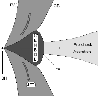
Figure 1: Schematic diagram of disc-jet system (with up-down symmetry) where the position of black hole (BH), shock location ($x_{s}$), CENBOL, centrifugal barrier (CB), funnel wall (FW) etc are shown. The dotted line is the axis of symmetry.

2.1 Equations for accretion

In the steady state, the dimensionless hydrodynamic equations of motion for accretion are (Chakrabarti, 1996),

the radial momentum equation :

$$u\frac{du}{dx}+\frac{1}{\rho}\frac{dP}{dx}-\frac{\lambda^{2}(x)}{x^{3}}+\frac{1}{2(x-1)^{2}}=0,$$

the baryon number conservation equation :

$$\dot{M}=2\pi\Sigma ux,$$

the angular momentum conservation equation :

$$u\frac{d\lambda(x)}{dx}+\frac{1}{\Sigma x}\frac{d}{dx}\left(x^{2}W_{x\phi}\right)=0,$$

and finally, the entropy generation equation :

$$uT\frac{ds}{dx}=-\frac{{\alpha}_{\Pi}}{\gamma}x(ga^{2}+\gamma u^{2})\frac{d\Omega}{dx},$$

where, variables $u$, $a$, $\rho$, $P$ and $\Omega(x)$, and $\lambda(x)$ in the above equations are the radial velocity, sound speed, density, isotropic pressure, angular velocity and specific angular momentum of the flow respectively. Here $\Sigma$ is vertically integrated density, $W_{x\phi}$($=-\alpha_{\Pi}\Pi$, $\Pi$ is the vertically integrated total pressure, $\alpha_{\Pi}$ is the viscosity parameter) denote the viscous stress, $s$ is the specific entropy of the flow, and $T$ is the local temperature. The disk is assumed to be in hydrostatic equilibrium in the vertical direction. Furthermore, $g=I_{n+1}/I_{n}$, $n=1/(\gamma-1)$ and $I_{n}=(2^{n}n!)^{2}/(2n+1)!$ (Matsumoto et al., 1984), and the adiabatic index $\gamma=4/3$ is used through out the paper.

2.2 Equations of motion for outflows

Figure 2: Jet geometry for $\lambda=1.75$. In figure $OA=r_{FW}$, $OC=r_{CB}$, $QC=x_{CB}$, $CM=y_{CB}$; $CM=BP(y_{j})=AN(y_{FW})$; $QA=x_{FW}$; $QB=x_{j}$; And $OB=r_{j}$. FW and CB are marked in the figure.

Numerical simulations by Molteni et al. (1996) suggests that the outflowing matter tends to emerge out between two surfaces namely, the funnel wall (FW) and the centrifugal barrier (CB). In Fig. 2, the schematic diagram of the jet geometry is shown. Geometric surfaces CB and FW are marked in the figure. The centrifugal barrier (CB) surface is defined as the pressure maxima surface and is expressed as

$$x_{CB}=\left[2\lambda^{2}r_{CB}(r_{CB}-1)\right]^{1/4},$$

where, $r_{CB}=\sqrt{x^{2}_{CB}+y^{2}_{CB}}{\equiv}$ spherical radius of CB. Here $x_{CB}$, $y_{CB}$ are the cylindrical radius and axial coordinate (i.e., height at $r_{CB}$) of CB. We compute the jet geometry with respect to $y_{CB}$ i.e., $y_{FW}=y_{j}=y_{CB}$, where $y_{FW}$ and $y_{j}$ are the height of FW and the jet at $r_{CB}$, respectively. The FW is obtained by considering null effective potential and is given by

$$x^{2}_{FW}=\lambda^{2}\frac{(\lambda^{2}-2)+\sqrt{(\lambda^{2}-2)^{2}-4(1-y^{2}_{CB})}}{2},$$

where, $x_{FW}$ is the cylindrical radius of FW. Using Eqs. (2a) and (2b), we estimate the cylindrical radius of the outflow

$$x_{j}=\frac{x_{FW}+x_{CB}}{2}.$$

The spherical radius of the jet is given by $r_{j}=\sqrt{x^{2}_{j}+y^{2}_{j}}$. In Fig. 2, $OB$ ($=r_{j}$) defines the streamline (solid) of the outflow. The total area function of the jet is obtained as,

$${\mathcal{A}=2\pi(x^{2}_{CB}-x^{2}_{FW})}$$

The integrated momentum balance equation for jet is given by,

$${\mathcal{E}}_{j}=\frac{1}{2}v^{2}_{j}+na^{2}_{j}+\frac{\lambda^{2}_{j}}{2x^{2}_{j}}-\frac{1}{2(r_{j}-1)},$$

where ${\mathcal{E}}_{j}$ and $\lambda_{j}$ are the specific energy and the angular momentum of the jet, respectively. The integrated continuity equation is,

$${\dot{M}}_{\rm out}=\rho_{j}v_{j}{\mathcal{A}},$$

and instead of the entropy generation equation we have the polytropic equation ($p_{j}=K_{j}\rho^{\gamma}_{j}$) of state for the jet. In Eqs. (3a-3b), the suffix ‘$j$’ indicates jet variables, where $v_{j}$, $a_{j}$, and $\rho_{j}$ are the velocity, the sound speed and the density of the jet.

3 Method

Since post-shock disc is the source of outflows, we are interested in only those accretion solutions which includes stationary shocks. A shocked accretion solution has two X-type critical points — inner ($x_{ci}$) and outer ($x_{co}$) critical points. Critical points are radial distances at which the gradient of velocity i.e., $du/dx{\rightarrow}0/0$. The accretion solution is solved by supplying $x_{ci}$ and angular momentum $\lambda_{i}$ at $x_{ci}$ and integrating the equations once from $x_{ci}$ inwards and then outwards [as in (Chakrabarti & Das, 2004)]. The conditions for steady shock require conservation of energy flux, mass flux, and momentum flux across the shock front [e.g., (Landau & Liftshitz, 1959)] and are given by,

$$\left[{\mathcal{E}}\right]=0;~{}~{}~{}~{}\left[\dot{M}\right]=0;~{}~{}~{}~{}\left[{\Pi}\right]=0.$$

In presence of mass loss, the condition for conservation of mass flux takes the following form,

$${\dot{M}}_{+}={\dot{M}}_{-}-{\dot{M}}_{\rm out}={\dot{M}}_{-}(1-R_{\dot{m}}),$$

where, subscripts “$-$” and “$+$” refer to quantities before and after the shock, respectively. The mass outflow rate $R_{\dot{m}}$ is the ratio between mass flux of the outflow (${\dot{M}}_{\rm out}$) and the pre-shock accretion rate (${\dot{M}}_{-}$). Using the above shock conditions, the pre-shock sound speed and bulk velocity can be expressed as,

$$a^{2}_{-}=\frac{C_{1}u_{-}}{g}-\frac{\gamma u^{2}_{-}}{g},$$

and,

$$\left[1-\frac{2\gamma}{g(\gamma-1)}\right]u^{2}_{-}+\frac{2C_{1}}{g(\gamma-1)}u_{-}+\left[\frac{\lambda^{2}_{s}}{x^{2}_{s}}-\frac{1}{x_{s}-1}-2{\mathcal{E}}_{s}\right]=0$$

where $C_{1}=(1-R_{\dot{m}})(ga^{2}_{+}+\gamma v^{2}_{+})/u_{+}$, and $({\mathcal{E}}_{s},\lambda_{s})$ are the energy and the angular momentum at the shock. As we integrate from $x_{ci}$ outwards, Eqs. (5a-b) are used to compute pre-shock flow variables. These pre-shock variables (i.e., $u_{-}$, $a_{-}$) are then used to find $x_{co}$. However, Eqs. (5a-b) show that the information of mass loss is in the shock condition itself. This implies that, in order to obtain shock the accretion-jet equations have to be solved simultaneously.

Jet equations are solved by employing the so-called ‘critical point analysis’ (Chakrabarti, 1990). We differentiate Eqs. (3a-3b) with respect to $r(=r_{CB})$, and obtain the expression for $dv_{j}/dr$. The critical point ($r_{jc}$) condition for jet is,

$$v^{2}_{jc}=a^{2}_{jc}=\left[\frac{1}{2(r_{jc}-1)^{2}}\left(\frac{dr_{j}}{dr}\right)_{r_{c}}-\frac{\lambda^{2}}{x^{3}_{jc}}\left(\frac{dx_{j}}{dr}\right)_{r_{c}}\right]\left[\frac{1}{{\mathcal{A}}_{c}}\left(\frac{d{\mathcal{A}}}{dr}\right)_{r_{c}}\right]^{-1},$$

Once the flow variables at the jet critical points are known, we integrate the jet equations from $r_{c}$ to the jet base ($x_{s}$).

The expression for $R_{\dot{m}}$ is calculated by assuming that jets are launched with the same density as the post-shock flow and is given by,

$$R_{\dot{m}}=\frac{{\dot{M}}_{\rm out}}{{\dot{M}}_{-}}=\frac{Rv_{j}(x_{s}){\mathcal{A}}(x_{s})}{4\pi\sqrt{\frac{2}{\gamma}}x^{3/2}_{s}(x_{s}-1)a_{+}u_{-}},$$

where the compression ratio is expressed as $R={\Sigma_{+}}/{\Sigma_{-}}$. The self-consistent method to obtain shocks in presence of mass loss is the following : initially the mass loss is not considered, and the shock is found out for accretion flows. Using $({\mathcal{E}}_{j},\lambda_{j})=({\mathcal{E}}_{s},\lambda_{s})$ as inputs, we solve the jet equations and calculate the values of jet variables at $r=x_{s}$. Once we obtain the value of $v_{j}$, ${\mathcal{A}}$ at $r=x_{s}$, we use Eq. (6) to calculate $R_{\dot{m}}$. The value of $R_{\dot{m}}$ is used in Eqs. (5a-5b), and the new shock location is obtained. We iterate this process till the solutions converge.

Figure 3: Upper panel: Inflow Mach number ($M=u/a$) with $log(x)$. The inflow parameters are $x_{ci}=2.445$, $\lambda_{i}=1.75$, and $\alpha_{\Pi}=0.002$, where, $x_{s}=19.21$, ${\mathcal{E}}_{s}=0.0014$, $\lambda_{s}=1.756$ $x_{co}=206.49$, $\lambda_{o}=1.772$. The dotted curve is the shock free solution. Lower panel: Outflow Mach number ($M_{j}=v_{j}/a_{j}$) with $log(x_{j})$, the outflow critical point $x_{jc}=81.26$ ($r_{jc}=346.18$), and the jet coordinates at the base is given by $x_{jb}=10.27$ ($r_{jb}=16.62$). The mass loss rate is $R_{\dot{m}}=0.055$.

4 Results

Supersonic matter, which was subsonic at the outer edge of the disc, suffers a discontinuous transition due to centrifugal barrier at shock ($x_{s}$) and becomes sub-sonic. A significant part of the post-shock matter is ejected as bipolar outflows due to excess thermal pressure at the shock and the rest enters into the black hole through $x_{ci}$. In Fig. 3, we present such a global inflow-outflow solution. In the top panel the Mach number of the accretion flow is plotted with $log(x)$. The solid curve represents shock induced accretion solution. The inflow parameters are $x_{ci}=2.445$ , $\lambda_{i}=1.75$, and $\alpha_{\Pi}=0.002$. In the lower panel, the outflow Mach number $M_{j}$ is plotted with $log(x_{j})$. In presence of mass loss ($R_{\dot{m}}=0.055$) the shock forms at $x_{s}=19.21$ (vertical line in the top panel), and the outflow is launched with energy and angular momentum at the shock (${\mathcal{E}}_{s},\lambda_{s}=0.0014,1.756$). The outflow is plotted up to its sonic point ($x_{jc}=81.26$).

Figure 4: Variation $R_{\dot{m}}$ with ${\mathcal{E}}_{\rm in}$, for ${\alpha}_{\Pi}=0$ (solid), $0.005$ (dotted), $0.01$ (dashed), and $0.015$ (dashed-dotted), $0.02$ (long-dashed) respectively, and $\lambda_{i}=1.75$.

We now present how the mass outflow rate is affected by viscosity in the disc. In Fig. 4, $R_{\dot{m}}$ is plotted with ${\mathcal{E}}_{\rm in}$ (the energy at $x_{ci}$), for a set of ${\alpha}_{\Pi}$. For instance, solid curve (${\alpha}_{\Pi}=0$) represents mass outflow rates for inviscid accretion. Other curves are obtained for the following values of ${\alpha}_{\Pi}$: $0.005$ (dotted), $0.01$ (dashed), and $0.015$ (dashed-dotted), and $0.02$ (long dash-dotted) respectively. All the curves are drawn for $\lambda_{i}=1.75$. We observe that higher energetic flow produces higher $R_{\dot{m}}$ for a given ${\alpha}_{\Pi}$. Conversely, for the same value of ${\mathcal{E}}_{\rm in}$ if $\alpha_{\Pi}$ is increased, then $R_{\dot{m}}$ is decreased significantly. It is to be noted that, for each ${\alpha}_{\Pi}$ there is a cut-off in $R_{\dot{m}}$ at the higher energy range, since standing shock conditions are not satisfied there. Non-steady shocks may still form in those regions, but investigation of such phenomena is beyond the scope of this paper.

Figure 5: (a) $R_{\dot{m}}$ vs $\alpha_{\Pi}$, for for $\lambda_{i}=1.8$ (solid), $1.775$ (dashed) and $1.75$ (dotted), respectively. Inner sonic points are $x_{ci}=2.313$, $2.375$, and $2.445$, respectively. (b) Variation of $x_{s}$ with $\alpha_{\Pi}$, $\lambda_{i}=1.75$ $x_{ci}=2.445$. Dotted curve represents solution without mass loss, and solid represents $x_{s}$ with mass loss. (c) Variation $\lambda_{s}$ with $\alpha_{\Pi}$,$\lambda_{i}=1.75$ $x_{ci}=2.445$. (d) Variation ${\mathcal{E}}_{s}$ with $\alpha_{\Pi}$,$\lambda_{i}=1.75$ $x_{ci}=2.445$. (e) Variation of $R$ (dotted) and $v_{j}{\mathcal{A}}$ (solid) with $\alpha_{\Pi}$, $\lambda_{i}=1.75$, $x_{ci}=2.445$. (f) Variation of $x^{3/2}_{s}(x_{s}-1)$ (dotted) and $a_{s+}u_{-}{\times}5e+4$ (solid) with $\alpha_{\Pi}$, $\lambda_{i}=1.75$, $x_{ci}=2.445$.

In Fig. 5a, $R_{\dot{m}}$ is plotted with $\alpha_{\Pi}$, for $(x_{ci},\lambda_{i})=(2.313,1.8)$ (solid), $(2.375,1.775)$ (dashed) and $(2.445,1.75)$ (dotted), respectively. For a given $\alpha_{\Pi}$, $R_{\dot{m}}$ increases with higher $\lambda_{i}$. This suggests that outflows are primarily centrifugal pressure driven. However, $R_{\dot{m}}$ decreases drastically with $\alpha_{\Pi}$ for each of the curves. The question however is, why $R_{\dot{m}}$ decreases with $\alpha_{\Pi}$? We wish to discuss the underlying physics and consider a representative case [e.g., $(x_{ci},\lambda_{i})=(2.445,1.75)$]. In Fig. 5b, shock location ($x_{s}$) is plotted with $\alpha_{\Pi}$, for solutions without mass loss (dotted) and with mass loss (solid). As viscosity is increased the shock location is decreased. Generally, in presence of mass loss shock forms closer to the black hole. Mass loss reduces the post-shock pressure, and therefore the shock moves inwards to maintain pressure balance across it. However, the two curves tend to merge at higher $\alpha_{\Pi}$, which signifies that the mass loss decreases with $\alpha_{\Pi}$. In Figs. 5(c-d), $\lambda_{s}$ and ${\mathcal{E}}_{s}$ are plotted with $\alpha_{\Pi}$, respectively. In this case, $\lambda_{i}$ is same, therefore with increasing $\alpha_{\Pi}$ there is a moderate increase of $\lambda(x)$ as we integrate outwards, however, ${\mathcal{E}}(x)$ decreases sharply, which results in the lower value of $x_{s}$. The fractional increase of $\lambda_{s}$ is ${\sim}1.1\%$. The fractional decrease of ${\mathcal{E}}_{s}$ is ${\sim}8.2\%$. As $x_{s}$ moves inwards, the base area ${\mathcal{A}}|_{r=x_{s}}$ of the jet decreases, and consequently the base velocity ($v_{j}|_{r=x_{s}}$) of the jet also decreases, while the compression ratio ($R$) increases. In Fig. 5e, $v_{j}{\mathcal{A}}$ (solid) and $R$ (dotted) is plotted with $\alpha_{\Pi}$. The quantity $v_{j}{\mathcal{A}}$ decreases by $90\%$, while $R$ increases by mere $60\%$. From Eq. (6), we see that in the denominator of the expression for $R_{\dot{m}}$, there is a term $x^{3/2}_{s}(x_{s}-1)a_{+}u_{-}$. In Fig. 5f, both the quantities $x^{3/2}_{s}(x_{s}-1)$ (dotted) and $a_{+}u_{-}$ (solid) is plotted with $\alpha_{\Pi}$. The quantity $x^{3/2}_{s}(x_{s}-1)$ decreases by $37\%$ and $a_{+}u_{-}$ (multiplied by a factor $5{\times}10^{4}$ in the figure) increases by $42\%$. Therefore, as $x_{s}$ decreases, the decrease of $v_{j}{\mathcal{A}}$ dominates all other quantities in Eq. (6), and hence $R_{\dot{m}}$ decreases with the increasing $\alpha_{\Pi}$. In Figs. 5(b-f), we have fixed ($\lambda_{i},x_{ci}$), and increased $\alpha_{\Pi}$ to see how viscosity affects shock and consequently $R_{\dot{m}}$. If one increases $\alpha_{\Pi}$ for fixed ($\lambda_{i},x_{ci}$), then ${\mathcal{E}}_{\rm in}$ will decrease anyway [e.g., Fig. (1c) of Chakrabarti & Das 2004], hence ${\mathcal{E}}_{s}$ will be lower for higher $\alpha_{\Pi}$. In other words, we have studied less energetic accretion flows though we have increased the $\alpha_{\Pi}$ parameter, and saw that for such flows increasing viscosity parameter decreases the shock location and therefore the mass outflow rate. The question however is, what happens to flows starting with same outer boundary conditions, as viscosity is increased?

In Fig. 6, the variation of $M$ (upper panel), $\lambda$ (middle panel), and ${\mathcal{E}}$ (lower panel) with $log(x)$ is presented. The flow is launched at the outer edge ($x_{\rm inj}=200$) with energy and angular momentum corresponding to $({\mathcal{E}}_{\rm inj},\lambda_{\rm inj})=(0.002,1.75)$. For inviscid case, the shock forms at $x_{s}=20.3$ (dashed) and mass outflow rate is calculated to be $R_{\dot{m}}=0.093$. As viscosity is incorporated (${\alpha}_{\Pi}=0.003$; dotted), the shock forms at $x_{s}=11.65$ and the outflow rate is reduced to $R_{\dot{m}}=0.07$. As viscosity is enhanced, ${\mathcal{E}}(x)$ is increased and $\lambda(x)$ is decreased along the flow. At the shock, the effect of energy increment, cannot compensate the effect due to angular momentum reduction. This weakens the centrifugal barrier and causes the shock to move inward. As shock moves inwards the jet-base area decreases, which reduces the mass outflow rate.

Figure 6: Variation of $M$ (upper panel), $\lambda$ (middle panel), ${\mathcal{E}}$ (lower panel) with $log(x)$, for ${\alpha}_{\Pi}=0$ (dashed) and ${\alpha}_{\Pi}=0.003$ (dotted). The outer edge quantities are $x_{\rm inj}=200$, $({\mathcal{E}}_{\rm inj},\lambda_{\rm inj})=(0.002,1.75)$. The shocks are $x_{s}=20.3$ (dashed) and $x_{s}=11.65$ (dotted).

Figure 7: Variation of $\tau$ with $(x)$, for $({\alpha}_{\Pi},R_{\dot{m}})=(0,0)$ (solid), $({\alpha}_{\Pi},R_{\dot{m}})=(0,0.093)$ (dotted), $({\alpha}_{\Pi},R_{\dot{m}})=(0.003,0)$ (dashed), and $({\alpha}_{\Pi},R_{\dot{m}})=(0.003,0.0.07)$ (dashed-dotted). The outer edge quantities are $x_{\rm inj}=200$, $({\mathcal{E}}_{\rm inj},\lambda_{\rm inj})=(0.002,1.75)$. Here $\tau$ is plotted for CENBOL.

So far, we have shown that the mass outflow rates strongly depends on shock location $x_{s}$, and formation of shock itself depends crucially on the viscosity parameter. We have also shown that shocks form closer to the black hole for viscous flows than in inviscid accretion flow. However, we are yet to comment on the observational consequence of such phenomena. Admittedly, it is beyond the scope of the present paper to compute the detailed spectrum of the flow, but we would like to make some qualitative remarks on the spectral properties of such flows. It is to be remembered, Chakrabarti & Titarchuk (1995) showed that hard power law photons were generated at CENBOL by inverse-Comptonization of soft photons from the pre-shock region of the disc. Thus we calculate the optical depth of the CENBOL, as this provides a qualitative understanding of the nature of the spectrum. The definition of the optical depth for photons entering the CENBOL is given by,

$$\tau(x)={\int}^{x}_{x_{s}}\kappa\rho dx^{\prime},$$

where, $\kappa$ is the opacity assuming Thompson scattering cross-section, and $\rho$ is the density of the flow. We consider matter with identical outer boundary conditions $(x_{\rm inj},{\mathcal{E}}_{\rm inj},\lambda_{\rm inj})=(200,0.002,1.75)$. The mass accretion rate at $x_{\rm inj}$ is ${\dot{M}}_{-}=0.3{\dot{M}}_{\rm Edd}$, and the central mass is $M_{BH}=10M_{\odot}$. In Fig. 7, $\tau(x)$ is plotted only for the post-shock disc with $({\alpha}_{\Pi},R_{\dot{m}})=(0,0)$ (solid), $(0,0.093)$ (dotted), $(0.003,0)$ (dashed), and $(0.003,0.07)$ (dashed-dotted), respectively. For the most simplified case (solid), the shock is at $x_{s}=25$, and the optical depth $\tau{\sim}1$ is at $8r_{g}$. Therefore most of the soft photons entering the CENBOL fails to sample the inner part of the disc. In presence of mass loss (dotted), the density of the CENBOL is lowered which reduces its optical depth. For viscous flow (dashed), optical depth is much lower compared to the inviscid flow (solid) as the shock forms ($x_{s}=14.2$) closer to the black hole. If we allow mass loss (dashed-dotted), the optical depth is reduced further. Therefore, most of the soft photons coming from the pre-shock region could interact with the hot electrons of the inner part of the disc ($\tau\sim 1$ at $x{\lower 2.15277pt\hbox{$\;\buildrel<\over{\sim}\;$}}4r_{g}$) and there by cool it. A cooler CENBOL will evidently produce softer spectrum compared to the inviscid case. Chakrabarti (1998) calculated spectrum of a inviscid disc which is loosing mass from the post-shock region, and indeed he found that the spectrum softens, which correspond to solutions similar to the dotted curve. From our self-consistent study, we predict that the twin effects of viscosity and mass loss will soften the spectrum even further.

5 Concluding Remarks

Early studies of transonic accretion flow showed the existence of standing or oscillating shocks (Chakrabarti, 1989). The presence of shocks were also thought to be the real cause behind hard state of the disc spectrum (Chakrabarti & Titarchuk, 1995), and also generating outflows (Chakrabarti, 1999). Studies of shocks in viscous accretion disc were also undertaken, but were confined to obtain the global solution for accretion flows with or without shocks and/or the detailed study of the parameter space (Chakrabarti, 1996; Chakrabarti & Das, 2004). Important as they are, since a proper understanding enhances the grasp on the physics of such flows, no attempts have been undertaken to link these viscous flows with observables such as outflows and spectrum. In this paper we have extended our earlier computation of mass loss (Das et al., 2001), by employing the knowledge of viscous disc solutions (Chakrabarti & Das, 2004). In the earlier paper (Das et al., 2001), the disc was considered to be inviscid and the jet was non-rotating. Furthermore, the shock condition was not modified for mass loss. Presently, we have included viscosity and considered rotating outflows, in particular we have concentrated on studying how viscosity affects shocks and in turn, how shocks affect the mass outflow rates.

We have shown that mass loss from the post-shock disc reduces post-shock total pressure, and hence the shock front moves towards the black hole. We have also shown that the mass outflow rate depends on the energy, as well as the angular momentum of the flow, and increasing both, in turn, increases the mass outflow rate. However, less energetic accretion will produce lower mass outflow rates, even though angular momentum is increased outward, by increasing the viscosity parameter.

More interestingly, we have shown that outflow rate decreases with the increase of viscosity parameter for flows with same outer boundary conditions. This is due to the weakening of centrifugal barrier with the increase of viscosity parameter. We have also shown that the post shock optical depth decreases in presence of viscosity and mass loss, which may soften the emitted spectrum. A detailed study of spectrum from such viscous discs, by including cooling processes is under consideration and will be reported elsewhere.

References

- Chakrabarti (1989) Chakrabarti, S. K. 1989, ApJ 347, 365 (C89).
- Chakrabarti (1990) Chakrbarti, S. K. 1990, Theory of Transonic Astrophysical Flows, World Scientific Publishing, Singapore.
- Chakrabarti & Titarchuk (1995) Chakrabarti, S. K., Titarchuk, L., 1995, ApJ 455, 623.
- Chakrabarti (1996) Chakrabarti, S. K. 1996, ApJ, 464, 664.
- Chakrabarti (1998) Chakrabarti, S. K., 1998, Ind. Journ. Phys. 72, 565.
- Chakrabarti (1999) Chakrabarti, S. K., 1999, A&A 351, 185.
- Chakrabarti & Das (2004) Chakrabarti, S. K., Das, S., 2004, MNRAS, 349, 649.
- Chakrabarti & Mandal (2006) Chakrabarti, S. K., Mandal, S., 2006, ApJL, 642, 49.
- Das & Chakrabarti (1999) Das, T. K., Chakrabarti, S. K., 1999, Class. Quant. Grav. 16, 3879.
- Das et al. (2001) Das, S., Chattopadhyay, I., Nandi, A., Chakrabarti, S. K., 2001a, A&A 379, 683.
- Gallo et al. (2003) Gallo, E., Fender, R. P., Pooley, G. G., 2003, MNRAS, 344, 60.
- Landau & Liftshitz (1959) Landau, L. D., Liftshitz, E. D., 1959, Fluid Mechanics, Pergamon, New York.
- Matsumoto et al. (1984) Matsumoto, R, Kato, S., Fukue, J., Okazaki A. T., 1984, PASJ, 36, 71.
- Molteni et al. (1994) Molteni, D., Lanzafame, G., Chakrabarti, S. K., 1994, ApJ, 425, 161.
- Molteni et al. (1996) Molteni, D., Ryu, D., Chakrabarti, S. K., 1996, ApJ, 470, 460.
- Paczyński & Wiita (1980) Paczyński, B., Wiita, P., 1980, A&A 88, 23