Behaviour of dissipative accretion flows around black holes

Abstract

We investigate the behaviour of dissipative accreting matter close to a black hole as it provides the important observational features of galactic and extra-galactic black holes candidates. We find the complete set of global solutions in presence of viscosity and synchrotron cooling. We show that advective accretion flow can have standing shock wave and the dynamics of the shock is controlled by the dissipation parameters (both viscosity and cooling). We study the effective region of the parameter space for standing as well as oscillating shock. We find that shock front always moves towards the black hole as the dissipation parameters are increased. However, viscosity and cooling have opposite effects in deciding the solution topologies. We obtain two critical cooling parameters that separate the nature of accretion solution.

1 Introduction

Accretion process around compact objects has been extensively studied during last three decades. Several attempts have been made for the development of the theory of accretion disc. The standard theory of thin accretion disc provides a self-consistent solution of Keplerian disc model (Shakura & Sunyaev 1973, hereafter SS73). Soon after the standard disc model was proposed people realized that the disc are not Keplerian everywhere, particularly in the radiation pressure dominated region (Lightman & Eardley 1974, Chakrabarti 1996a). In addition, this model (SS73) was unsuccessful to explain the origin of observed high energy radiation. A possible solution immediately came in the literature (Sunyaev & Titarchuk, 1985) that disc may possess a Compton cloud which must inverse Comptonize the Keplerian soft photons to produce the hard X-rays. Incidentally, Chakrabarti & Molteni (1995) and Lanzafame et al. (1998) showed by numerical simulation that angular momentum distribution purely depends on the viscosity prescription under consideration and remains sub-Keplerian close to the black hole as flow must cross the horizon super-sonically (Chakrabarti, 1990). Recent observations do support the fact that sub-Keplerian matter may be present in accretion disc (Smith et al. 2001, Smith et al. 2002).

In an earlier study, Chakrabarti (Chakrabarti 1989, Chakrabarti 1990) extensively discussed the transonic properties of inviscid, polytropic flows and showed that standing shock waves can form for a large region of parameter space spanned by the specific energy and specific angular momentum of the flow. Various authors (Nobuta & Hanawa 1994, Yang & Kafatos 1995, Lu & Yuan 1997, Gu & Lu 2004, Fukumura & Tsuruta 2004) found the existence of standing shock waves in different astrophysical contexts. In an accretion process around a black hole, flow is sub-sonic at a large distance and crosses the horizon super-sonically. Thus, black hole accretion is necessarily transonic. For a given set of input parameters, namely specific energy and specific angular momentum, the flow passes through the outer sonic point $(x_{out})$ and remains super-sonic as it proceeds inwards. At a distance $x_{s}~{}(<x_{out})$, flow is virtually stopped due to the resistance offered by the centrifugal barrier and consequently a shock is formed. The post-shock flow momentarily becomes sub-sonic and flow temperature increases in this region as the kinetic energy of the flow is converted in to thermal energy. Subsequently, flow picks up its velocity as it approaches black hole horizon and eventually crosses the horizon supersonically after passing through the inner sonic point $(x_{in})$.

The first global and fully self-consistent solution of viscous transonic flows including advection in the optically thin and thick limit was obtained by Chakrabarti (Chakrabarti 1990 and references there in) where it was assumed that Keplerian flow at the outer edge can become sub-Keplerian at the inner part of the disc. Later, Chakrabarti & Das (2004a) presented a complete classification of global solutions of viscous transonic flow according to solution topologies and identified the region in the parameter space where the flow possesses multiple sonic points. Within this region, if the viscosity parameter is below its critical value $(\alpha_{\Pi}<\alpha_{\Pi s})$, there are solutions where Rankine-Hugoniot shock conditions (Landau & Lifshitz 1959, hereafter RHCs) are satisfied and standing shock is formed due to centrifugal barrier (Chakrabarti 1990, Chakrabarti 1996b, Chakrabarti & Das 2004a). When viscosity is increased beyond a critical value, shocks disappear (see Fig. 12 of Chakrabarti & Das 2004a). Of course, the viscosity parameter strongly depends on the model parameters such as sonic point location and angular momentum at the inner boundary. The importance of critical viscosity is being reconsidered by Gu & Lu (2004) where a ‘qualitative’ estimate of critical viscosity for standing shock ($\alpha_{\Pi s}\leq 0.5$) was reported. Furthermore, many authors pointed out that shocks may undergo either radial or vertical or non-axisymmetrical oscillations (Molteni et al. 1999, Gu & Foglizzo 2003) although they are generally never ruined by these oscillations. In Das & Chakrabarti (2004), Bremsstrahlung cooling also added keeping in mind that it is a very inefficient cooling process (Chattopadhyay & Chakrabarti, 2000) and complete set of global solutions of viscous transonic flow with and without shocks were presented. The hot and dense post shock flow which basically acts as a ‘boundary layer’ of the black holes could be the natural site of the hot radiation in the accretion disc and is considered to be a powerful tool in understanding the important astrophysical phenomena such as the spectral properties of black holes (Chakrabarti & Titarchuk 1995, Chakrabarti et al. 1996c, Ebisawa et al. 1996, Mandal & Chakrabarti 2005), the source of quasi-periodic oscillation (QPO) of the hard X-rays from the black hole candidates (Molteni et al. 1996, Ryu et al. 1997, Chakrabarti et al. 2004b) and the generation of accretion-powered relativistic bipolar outflows/jets (Das et al. 2001a and references there in). Recently, Chakrabarti & Mandal (2006) reported that this boundary layer could be responsible for the spectral state transition in at least some of the black hole candidates, such as Cyg X1. Also, Fender et al. (2000) and Dhawan et al. (2000) showed that outflow could be produced from the same region that emits the Comptonized photons. A globally complete Inflow-Outflow solution of viscous accretion flow is also found by Chattopadhyay & Das (2006).

Being motivated by the above arguments, in the present paper, we wish to follow up the stationary, axisymmetric, viscous accretion solutions around a Schwarzschild black hole in presence of Synchrotron cooling. Such dissipative viscous accreting flow have not yet been explored in the literature. The space-time geometry around a non-rotating black hole is satisfactorily described by pseudo-Newtonian potential (Paczyński & Wiita, 1980). We consider similar viscosity prescription as in Chakrabarti (1996b). We calculate all relevant dynamical and thermodynamical flow variables and extensively study the dependence of such variables on the the flow parameters like specific energy, specific angular momentum and the dissipation parameters (Synchrotron cooling and/or viscosity parameters). We identify the solution topologies which are essential for shock formation. In the present study, we concentrate on the non-dissipative shocks that preserve the energy across it. In a generalized accretion flow, cooling reduces the energy of the flow while viscosity not only tends to heat the flow but lowers the flow angular momentum as flow accretes. Thus the effect of viscosity and Synchrotron cooling on the dynamical structure of the accretion flow are expected to be different. Since shock has observational consequences as mentioned above, it is, therefore, pertinent to know how the dynamics of shock is controlled by the dissipation parameters. In particular, whether shock front moves inward or outward if the dissipation is increased. In the present paper, we attempt to discuss this issue extensively. Moreover, we find that shock waves, standing or oscillating, are still formed even when at very high dissipation limit. In this paper, we provide a useful formalism to study the dissipative transonic accretion flow which is valid for a wide range in accretion rates.

We arrange the paper in the following way: in the next section, we present the governing equations. In §3, we perform sonic point analysis. In §4, we study the global solution topologies and classify the parameter space for solutions having multiple sonic points as a function of cooling parameter. In §5, we study the dynamics of shock and dependence of shock properties on the the flow parameters. In §6, we classify the the parameter space as a function of cooling parameter in terms of whether shocks, standing or oscillating, will form or not. In §7, we quantify the critical cooling parameters. Finally, in §8, we make concluding remarks.

2 Basic hydrodynamic equations

We begin with a stationary, thin, viscous, axisymmetric accretion flow on to a Schwarzschild black hole. In this paper, we consider pseudo-Newtonian potential introduced by Paczyński & Wiita (1980) to solve the problem instead of using full general relativity, which allows us to use the Newtonian concept at the same time retaining all the salient features of the space-time geometry around a non-rotating black hole. The governing equations for the accreting flow are written on the equatorial plane of the accretion disc. The flow equations are made dimensionless by considering unit of length, time and the mass as $r_{g}=2GM_{BH}/c^{2}$, $2GM_{BH}/c^{3}$ and $M_{BH}$ respectively where, $G$ is the gravitational constant, $M_{BH}$ is the mass of the black hole and $c$ is the velocity of light respectively. Henceforth, all the flow variables are expressed in geometrical units.

In the steady state, the hydrodynamics of the axisymmetric accreting matter around a non-rotating black hole in the pseudo-Newtonian limit is given by (Chakrabarti, 1996b),

(i) the radial Momentum equation :

$$\vartheta\frac{d\vartheta}{dx}+\frac{1}{\rho}\frac{dP}{dx}-\frac{\lambda^{2}}{x^{3}}+\phi(x)=0,$$

(ii) the mass flux conservation equation :

$$\dot{M}=\Sigma\vartheta x$$

(iii) the angular momentum conservation equation :

$$\vartheta\frac{d\lambda(x)}{dx}+\frac{1}{\Sigma x}\frac{d}{dx}\left(x^{2}W_{x\phi}\right)=0,$$

and finally,

(iv) the entropy generation equation :

$$\Sigma\vartheta T\frac{ds}{dx}=\frac{h\vartheta}{\gamma-1}\left(\frac{dP}{dx}-\frac{\gamma P}{\rho}\frac{d\rho}{dx}\right)=Q^{+}-Q^{-}.$$

The local variables $x$, $\vartheta$, $\rho$, $P$ and $\lambda$ in the above equations are the radial distance, radial velocity, density, isotropic pressure and the angular momentum of the flow respectively. Here, $\phi(x)=-\frac{1}{2}(x-1)^{-1}$ denotes the pseudo-Newtonian potential and $\gamma$ is the adiabatic index of the flow. Furthermore, $s$ and $T$ are the specific entropy and the local temperature of the flow, $\Sigma$ is the vertically integrated density and $W_{x\phi}$ is the viscous stress. Here, $Q^{+}$ and $Q^{-}$ represent the energy gained and lost by the flow respectively, and ${\dot{M}}$ is the mass accretion rate. In our model, the accreting flow is assumed to be in hydrostatic equilibrium in the vertical direction. The half thickness of the disc is then obtain by equating the vertical component of the gravitational force and the pressure gradient force as,

$$h(x)=ax^{1/2}(x-1).$$

where, $a$ denotes the adiabatic sound speed defined as $a=\sqrt{\gamma P/\rho}$. In this paper, we use the similar viscosity prescription of Chakrabarti (1996b). In this prescription, viscous stress remain continuous across the axisymmetric shock wave for flows with significant radial motion.

Now we simplify the entropy equation (Eq. 4) as:

$$\frac{\vartheta}{\gamma-1}\left[\frac{1}{\rho}\frac{dP}{dx}-\frac{\gamma P}{\rho^{2}}\frac{d\rho}{dx}\right]=\frac{Q^{-}-Q^{+}}{\rho h}=\Lambda-\Gamma,$$

where, $\Gamma(=Q^{+}/\rho h)$ denotes the energy gained due to the viscous heating and is obtained as,

$$\Gamma=\frac{-\alpha_{\Pi}I_{n}x}{\gamma}\left(ga^{2}+\gamma\vartheta^{2}\right)\frac{d\Omega}{dx}.$$

Here, $\alpha_{\Pi}$ is the viscosity parameter and $\Omega(x)$ is the angular velocity of the accreting matter at a radial distance $x$. The polytropic index is denoted by $n=(1-\gamma)^{-1}$. $I_{n}$ and $I_{n+1}$ come from the vertically averaged density and pressure (Matsumoto et al., 1984) and $g=I_{n+1}/I_{n}$. The term $\Lambda(=Q^{-}/\rho h)$ represents the energy loss by the flow. In the present analysis, we ignore energy loss due to Bremsstrahlung cooling as it is not very efficient cooling process (Chattopadhyay & Chakrabarti, 2000) and include synchrotron cooling only. Indeed, magnetic field is ubiquitous inside the accretion disc and therefore, the ionized flow in turn should emit synchrotron radiation that may cool down the accreting flow significantly. Since the satisfactory description of magnetic field inside the accretion disc is not well understood, we thus assume only random or stochastic magnetic field. Such magnetic field may or may not be in equipartition with the accretion flow. We define a parameter $\eta$ as the ratio of the magnetic pressure and the thermal pressure of the flow under consideration and is given by,

$$\eta=\frac{B^{2}\mu m_{p}}{8\pi\rho k_{B}T_{p}}$$

where, $B$ denotes the magnetic field strength, $k_{B}$ is the Boltzmann constant, $\mu$ is the mean molecular weight and $m_{p}$ is the mass of the proton respectively. In general, $\eta\mathrel{\hbox{\hbox to0.0pt{\hbox{\lower 4.0pt\hbox{$\sim$}}\hss}\hbox{$<$}}}1$ which ensures that magnetic fields definitely remain confined within the disc (Mandal & Chakrabarti, 2005). While obtaining Eq. (7), we consider the gas is assumed to obey an ideal equation of state. In an electron-proton plasma, we use equipartition magnetic field (Eq. 7) to account for the non-dimensional synchrotron cooling effect which is obtained in a convenient form as (Shapiro & Teukolsky, 1983):

$$\Lambda=\frac{Sa^{5}}{\vartheta x^{3/2}(x-1)},$$

with

$$S=7.5424\times\frac{\eta\beta{\dot{M}}\mu^{2}e^{4}}{m_{e}^{3}\gamma^{5/2}}\frac{1}{2GM_{BH}c^{3}},$$

where, $e$ and $m_{e}$ represent the charge and mass of the electron respectively. We estimate electron temperature from the expression $T_{e}=\sqrt{m_{e}/m_{p}}T_{p}$ (Chattopadhyay & Chakrabarti, 2002) and use it to obtain Eq. (8). Here, $\beta$ is a dimensionless cooling parameter that controls the efficiency of cooling. When $\beta\rightarrow 0$, the flow is heating dominated as it cools most inefficiently. In the present paper, we consider $\gamma=4/3$, $\eta=0.1$ and $\dot{M}=0.233\dot{M}_{Edd}$ for $10M_{\sun}$ black hole, until otherwise stated.

3 Sonic point analysis

We solve Eqs.(1-3, 4a) following the standard method of sonic point analysis (Chakrabarti, 1989). We calculate the radial velocity gradient as:

$$\frac{d\vartheta}{dx}=\frac{N}{D},$$

where, the Numerator $N$ is given by,

$$N=\frac{Sa^{5}}{x^{3/2}(x-1)}+\frac{\alpha^{2}_{\Pi}I_{n}(a^{2}g+\gamma\vartheta^{2})^{2}}{\gamma^{2}x}+\frac{\alpha^{2}_{\Pi}gI_{n}a^{2}(5x-3)(a^{2}g+\gamma\vartheta^{2})}{\gamma^{2}x(x-1)}$$

$$-\left[\frac{\lambda^{2}}{x^{3}}-\frac{1}{2(x-1)^{2}}\right]\left[\frac{(\gamma+1)\vartheta^{2}}{(\gamma-1)}-\frac{2\alpha^{2}_{\Pi}gI_{n}(a^{2}g+\gamma\vartheta^{2})}{\gamma}\right]$$

$$-\frac{\vartheta^{2}a^{2}(5x-3)}{x(\gamma-1)(x-1)}-\frac{2\lambda\alpha_{\Pi}I_{n}\vartheta(a^{2}g+\gamma\vartheta^{2})}{\gamma x^{2}}$$

and the denominator $D$ is,

$$D=\frac{2a^{2}\vartheta}{(\gamma-1)}-\frac{(\gamma+1)\vartheta^{3}}{(\gamma-1)}+\frac{\alpha^{2}_{\Pi}I_{n}\vartheta(a^{2}g+\gamma\vartheta^{2})}{\gamma}\left[(2g-1)-\frac{a^{2}g}{\gamma\vartheta^{2}}\right].$$

The gradient of sound speed is obtained as:

$$\frac{da}{dx}=\left(\frac{a}{\vartheta}-\frac{\gamma\vartheta}{a}\right)\frac{d\vartheta}{dx}+\frac{\gamma}{a}\left[\frac{\lambda^{2}}{x^{3}}-\frac{1}{2(x-1)^{2}}\right]+\frac{(5x-3)a}{2x(x-1)}$$

and similarly, the gradient of angular momentum is calculated as:

$$\frac{d\lambda}{dx}=\frac{\alpha_{\Pi}(a^{2}g+\gamma\vartheta^{2})}{\gamma\vartheta}-\frac{\alpha_{\Pi}x(a^{2}g-\gamma\vartheta^{2})}{\gamma\vartheta^{2}}\frac{d\vartheta}{dx}+\frac{2\alpha_{\Pi}axg}{\gamma\vartheta}\frac{da}{dx}$$

At the outer edge of the accretion disc, matter starts to accrete with almost negligible radial velocity and enters into the black hole with velocity of light. This indicates that ‘radial velocity gradient’ should be always real and finite to maintain the accretion flow smooth along the streamline. However, Eq. (10b) indicates that there may be some points where denominator ($D$) vanishes. Since the flow is smooth everywhere along the streamline, the point where denominator tends to zero, the numerator ($N$) must also vanish there. The point where both the numerator and denominator vanish simultaneously is called as critical point or sonic point. Setting $D=0$, one can easily obtain the expression for the Mach number $(M=\vartheta/a)$ at the sonic point as,

$$M(x_{c})=\sqrt{\frac{-m_{2}-\sqrt{m^{2}_{2}-4m_{1}m_{3}}}{2m_{1}}},$$

where,

$$m_{1}=\gamma^{2}\left[\alpha^{2}_{\Pi}I_{n}(2g-1)(\gamma-1)-(\gamma+1)\right]$$

$$m_{2}=2\gamma\left[\gamma+\alpha^{2}_{\Pi}I_{n}g(g-1)(\gamma-1)\right]$$

$$m_{3}=-\alpha^{2}_{\Pi}I_{n}g^{2}(\gamma-1)$$

In the weak viscosity limit, the Mach number at the sonic point becomes,

$$M(x_{c})=\sqrt{\frac{2}{\gamma+1}}$$

This result is exactly same as Chakrabarti (1989). This indicates that Mach number at the sonic point in presence of different cooling process remains same as in the case for the non-dissipative accretion flow. We obtain an algebraic equation for sound speed by using another sonic point condition $N=0$ which is given by,

$$F({\mathcal{E}}_{c},\lambda_{c},x_{c})={\mathcal{A}}a^{3}(x)+{\mathcal{B}}a^{2}(x)+{\mathcal{C}}a(x)+{\mathcal{D}}=0,$$

where,

$${\mathcal{A}}=\frac{S}{x^{3/2}(x-1)},$$

$${\mathcal{B}}=\frac{\alpha^{2}_{\Pi}I_{n}(g+\gamma M^{2})^{2}}{\gamma^{2}x}+\frac{\alpha^{2}_{\Pi}I_{n}g(5x-3)(g+\gamma M^{2})}{\gamma^{2}x(x-1)}$$

$$-\frac{M^{2}(5x-3)}{x(\gamma-1)(x-1)},$$

$${\mathcal{C}}=-\frac{2\lambda\alpha_{\Pi}I_{n}M(g+\gamma M^{2})}{\gamma x^{2}},$$

and

$${\mathcal{D}}=-\left[\frac{\lambda^{2}}{x^{3}}-\frac{1}{2(x-1)^{2}}\right]\left[\frac{(\gamma+1)M^{2}}{(\gamma-1)}-\frac{2\alpha^{2}_{\Pi}gI_{n}(g+\gamma M^{2})}{\gamma}\right].$$

We solve Eq. (14) analytically (Abramowitz & Stegun, 1970) and obtain the sound speed at the sonic point by knowing the flow parameters. Depending on the input parameters, a non-dissipative flow may have maximum of four sonic points (Das et al., 2001b). Among them, one always lies inside the horizon and the others, if they at all exist, remain outside the horizon. In our present analysis, we continue to use similar concept to obtain dissipative accretion solutions (Chakrabarti & Das, 2004a). The nature of sonic points and its detailed properties could be easily understood with the extensive study of Eq. (10) when the flow parameters are known. Infact, nature of sonic points depends on the value of velocity gradients at the sonic point. In general, $d\vartheta/dx$ possesses two values at the sonic point. One of them is for accretion flow and the other is valid for wind. When both the derivatives are real and is of opposite signs, the sonic point is saddle type or X-type. Nodal type sonic point is obtained when both the derivatives are real and is of same sign. If the derivatives are complex, the sonic point belongs to the class of spiral type or O-type. In the astrophysical context, saddle type sonic point has some special importance since transonic flows usually pass through it. In addition, in order to form a standing shock, the flow must have more than one saddle type sonic points among them the closest and furthest values corresponds to inner and outer X-type sonic points. The O-type sonic point which lies between the two saddle type sonic point is unphysical in the sense that no stationary solution passes through it.

4 Solution Topologies

To obtain a complete solution, one needs to supply the boundary values of energy, accretion rate and angular momentum of the flow for a given viscosity ($\alpha_{\Pi}$) and cooling parameter ($\beta$) and integrates Eqs.(10, 11, 12) simultaneously with the help of Eqs. (10a, 10b). Since black hole solution is necessarily transonic, flow must pass through the sonic points. In addition, flow presumably originates from the Keplerian disc ($x_{Kep}$) and it must carry angular momentum $\lambda(x_{Kep})$, a part of which is transported due to viscosity outwards and the other part is advected into the black hole through the sonic point. The distribution of the angular momentum from the inner edge of the disc to the $x_{Kep}$ is obtained from Eq. (12). Incidentally, the acceptable range of angular momentum at the inner edge of the disc and the inner sonic point location of the accreting solution is very small (say, $1.5\mathrel{\hbox{\hbox to0.0pt{\hbox{\lower 4.0pt\hbox{$\sim$}}\hss}\hbox{$<$}}}\lambda_{in}\mathrel{\hbox{\hbox to0.0pt{\hbox{\lower 4.0pt\hbox{$\sim$}}\hss}\hbox{$<$}}}2$ and $2\mathrel{\hbox{\hbox to0.0pt{\hbox{\lower 4.0pt\hbox{$\sim$}}\hss}\hbox{$<$}}}x_{in}\mathrel{\hbox{\hbox to0.0pt{\hbox{\lower 4.0pt\hbox{$\sim$}}\hss}\hbox{$<$}}}4$, Chakrabarti 1989, Chakrabarti & Das 2004a). We, thus, choose inner sonic point location $x_{in}$ and the angular momentum at the inner sonic point $\lambda(x_{in})$ (hereafter, we denote it as $\lambda_{in}$) as input parameters instead of the aforementioned energy and the angular momentum flow at the outer edge of the disc. We once integrate Eqs.(10, 11, 12) inwards upto the horizon and again outwards to a large distance $(\sim x_{Kep})$ to obtain a complete transonic solution. A comprehensive study of viscous transonic flow is already presented by Chakrabarti & Das (2004a) and therefore, in the current paper, we mainly concentrate on the properties of accreting solution in presence of synchrotron cooling, until otherwise stated.

4.1 Behavior of Global Solutions

In order to obtain a shock solution around a black hole, accreting flow must possess multiple saddle type sonic points. Shock joins different solution branches, one passes through the inner sonic point and the other passes through the outer sonic point. Thus, it is important to understand the nature of solution trajectories in presence of energy dissipation.

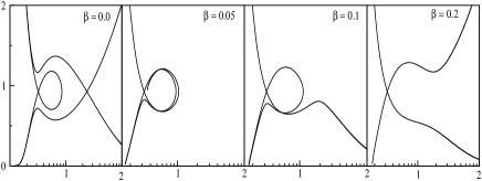
Figure 1: Global solution topologies in presence of Synchrotron cooling. In each boxes, variation of Mach number is plotted with logarithmic radial distance. Flow parameters are $x_{in}=3.107$, $\lambda_{in}=1.6$. Cooling parameters are marked in the figure.

Fig. 1 shows examples of global solutions of inviscid accretion flow passing through the inner sonic point. Each box depicts Mach number ($M=\vartheta/a$) variation as a function of the logarithmic radial distance. We write the cooling parameter $\beta$ in each box (marked as 0.0, 0.05, 0.1 and 0.2). The other flow parameters for Fig. 1 are chosen as $x_{c}=3.107$, $\lambda_{in}=1.6$ and $n=3$ respectively. Here, all the sonic points are saddle type, and the solutions may or may not have shock depending on its global solution topologies. In the first column, the flow is dissipation free and the sonic points are uniquely determined as energy and angular momentum are conserved all throughout. Accreting solutions of this kind deviate from the Keplerian disc at the outer part of the disc and enter into black hole super-sonically with the radial velocity equal to the velocity of light after crossing the outer sonic point. Another possibility is that super-sonic flow may suffer shock transition at sub-sonic branch, if shock conditions hold (see §5) and crosses the black hole horizon after passing through the inner sonic point as it has to satisfy the ‘super-sonic’ inner boundary condition at the horizon. In the second column, cooling is incorporated and the flow topologies passing through the inner sonic point start to open up. The outer sonic point, if it exits, can not be determined unless a shock is formed as energy of the flow is not conserved here. When cooling is increased further, the flow topologies are completely opened up (third and fourth column) and they leave the accretion shock regime. In this particular situation, flow deviates from the Keplerian disc far away from the black hole and enters into it straight away through the inner sonic point. So, for a given set of flow parameters, there must be a critical cooling parameter $(\beta_{cc})$ for which closed topologies passing through the same inner sonic point become open topologies. An exhaustive discussion of critical cooling parameter will be presented in §7.

4.2 Description of the parameter space

Figure 2: Classification of parameter space for closed topologies passing through the inner sonic point. The region bounded by different curve is obtained by using different cooling factor [$\beta=0.0$ (solid), $\beta=0.00787$ (dotted), $\beta=0.0787$ (dashed) and $\beta=0.393$ (dot-dashed)]. Notice that, parameter space gradually shrinks with the increase of cooling factor.

In order to understand the dissipative accretion flow, here, we classify the parameter space as a function of the cooling parameter in the $\mathcal{E}_{in}$-$\lambda_{in}$ plane where $\mathcal{E}_{in}$ denotes the energy of the flow at the inner sonic point $(x_{in})$. Infact, in a cooling dominated inviscid accretion flow, angular momentum remain conserved along the streamline of the flow. In Fig. 2, we have identified the region of the parameter space for closed spiraling accretion solution which passes through the inner sonic point as in panel 1-2 of Fig. 1. Accretion flows of this kind possess multiple sonic points and flow may suffer shock transition if the outer sonic point exits. The shock would be stationary or oscillating depending on whether the Rankine-Hugoniot relation is satisfied or not. The region bounded by the solid curve is obtained for dissipation free ($\beta=0$) accretion flow and it coincides with the result of Chakrabarti (1989). The dotted, dashed and the dot-dashed regions are obtained for cooling parameters $\beta=0.00787,0.0787$ and $0.393$ respectively. For higher $\beta$, the parameter space for closed topologies passing through the inner sonic point reduces in both lower and higher angular momentum sides. This is not surprising, since an increase of cooling induces damping inside the flow which reduces the number the sonic points for the same set of initial parameter as seen in Fig. 1. With the rise of $\beta$, the effective region of parameter space for the closed topologies gradually shrinks and disappears completely when the critical cooling $(\beta_{cc})$ is reached.

5 Shock Solutions and classification of parameter space

The existence of shock waves in accretion flow has been reported in many astrophysical context and the thermodynamical properties of shock waves like its location, strength and compression ratio could be determined exactly by using the RHCs. In the present study, we continue to use similar viscosity prescription as in Chakrabarti (1996b) that maintains viscous stress $(W_{x\phi})$ to be continuous across the shock in presence of significant radial motion. We compute the shock locations following an useful technique first presented by Chakrabarti & Das (2004a) for dissipative accretion flows.

5.1 Shock Dynamics and Shock properties

Figure 3: A complete accretion solution topology drawn with standing shocks ($x_{s}=23.83$). See text for details.

In Figure 3, we present a complete solution of vertically averaged flow where a shock wave connects two solution branches—one passing through the outer sonic point (O) and the other passing through the inner sonic point (I). In this figure, we plot the Mach number variation with the logarithmic radial distance. The flow parameters are chosen as $x_{in}=2.5308,\lambda_{in}=1.725$ and $\beta=0.0157$ respectively. Sub-sonic accretion flow crosses the outer sonic point at $x_{out}=80.07$ and makes discontinuous transition ($shock$) at $x_{s}=23.82$ before entering into the black hole. The shock location is shown by vertical dotted line. The exact location of the shock is obtained by solving Rankine-Hugotinot relations. In the present study, shock is assumed to be thin and non-dissipative. In addition, we ignore the presence of any excess sources of torque at the shock, that maintains the continuity of angular momentum across it. At the shock, entropy is generated which is subsequently advected into the black hole.

Figure 4: Plot of Mach number with the logarithmic radial distance. Flows with same energy $\mathcal{E}_{inj}=3.3663\times 10^{-3}$ and angular momentum $\lambda_{inj}=1.725$ at the outer edge $x_{inj}=145$ are injected with different dissipation parameters. Dissipation parameters are marked in the figure. The corresponding shock locations are indicated by the vertical lines [$x_{s}=25.99$ (solid), $x_{s}=20.6$ (dashed), $x_{s}=22.94$ (dotted) and $x_{s}=18.62$ (dot-dashed),].

In Fig. 4, we have shown how the shock location (indicated by the vertical lines) changes with the dissipation parameters ($\alpha_{\Pi}$ and/or $\beta$) for a given set of initial flow parameters. We inject matter sub-sonically at the outer edge of the disc $x_{inj}=145$ with local energy $\mathcal{E}(x_{inj})=3.3663\times 10^{-3}$ and angular momentum $\lambda(x_{inj})=1.725$. (hereafter, we denote them as $\mathcal{E}_{inj}$ and $\lambda_{inj}$ respectively). The sub-sonic flow first passes through the outer sonic point and becomes super-sonic. The Rankine-Hugoniot condition are satisfied here and eventually a shock is formed. The solid vertical line represents the shock location ($x_{s}=25.99$) for non-dissipation ($\alpha_{\Pi}=0$ and $\beta=0$) flow. As viscosity is turn on, shock front ($x_{s}=20.6$) moves forward denoted by the dashed vertical line. Due to viscosity, accreting flow losses angular momentum causing the reduction of centrifugal pressure and at the same time energy of the flow increases. At the shock, total pressure must be continuous and thus, the dynamics of the shock are mainly controlled by the resultant pressure across it. Since the shock moves in and as $\lambda(x)$ get reduced along the viscous flow, therefore, we can conclude that centrifugal force is the primary cause for shock formation. When synchrotron cooling is effective in an inviscid accretion flow, shock location ($x_{s}=22.94$) again proceeds towards the horizon depicted by vertical dotted line. In the pre-shock region, density and temperature are low and therefore, the effect of cooling is negligible (see below). The situation is completely opposite in the post-shock region and cooling reduces the post-shock pressure causing the shock to move forward further. This indicates that thermal pressure is also not less important in determining the final shock location. In a generalized accretion flow where both viscosity and cooling are present, shock location is predicted at $x_{s}=18.62$ for the same set of input parameter as above and is denoted by vertical dot-dashed line. In this particular case, shock front is shifted significantly due to combined effects of viscosity and cooling. When the mass loss from the viscous disc (Chattopadhyay & Das, 2006) is considered, shock is seen to form even closer to the black hole as some part of the accreted matter is ejected as outflows which reduces the post-shock pressure drastically.

Figure 5: The variation of (a) Flow temperature and (b) total Synchrotron loss (in geometric units) with radial distance.

In Fig. 5a, we have plotted the logarithmic proton temperature $(T=\mu m_{p}a^{2}/\gamma k_{B})$ of a weakly viscous flow as a function of the radial distance for the same set of input parameters as in Fig. 4 with $\beta=0.0236$. Clearly Fig. 5a indicates that post-shock temperature is much higher compared to the pre-shock temperature. This is because shock compresses the flow and makes it hotter. In particular, at the shock, flow temperature rises sharply as the kinetic energy of the flow converted to the thermal energy there. In Fig. 5b, we show how the total synchrotron loss (in logarithmic scale with geometric unit) vary with the radial distance for the same set of flow parameters as in Fig 5a. The net energy loss is negligible in the pre-shock region while it increases significantly as the post-shock flow advected towards the black hole.

Figure 6: (a) Variation of shock location with the cooling factor when the flows with identical angular momentum and energy are injected from a fixed outer boundary. Solid, dotted and dashed curves are drawn for flow with angular momentum $\lambda_{in}=1.7,1.725$ and $1.75$. Shock forms further for higher angular momentum flow suggests that shock are mainly centrifugally driven. In all cases, shock moves closer to the black hole as the cooling factor is increased. (b) Variation of compression ratio $(R=\Sigma_{+}/\Sigma_{-})$ with the cooling factor for same set of parameters as (a). Subscripts “+” and “-” refer to quantities before and after shock. Compression ratio monotonically increases in all the cases as the cooling factor is increased. (c) Variation of shock strength $(\Theta=M_{-}/M_{+})$ with the cooling factor for same set of parameters as (a). Shock strength gradually increases in all the cases as the cooling factor is increased.

Fig. 6a compares the shock locations as a function of the cooling parameter $\beta$ for different values of angular momentum $\lambda_{inj}$. In all the cases, the matter is injected at the outer edge of the disc $x_{inj}=145$. The solid curve is for $\lambda_{inj}=1.7$ and the dotted and dashed curve are for $\lambda_{inj}=1.725$ and $\lambda_{inj}=1.75$ respectively. The corresponding local energies at the injection point are $\mathcal{E}_{inj}=2.5156\times 10^{-3}$ (solid), $3.3663\times 10^{-3}$ (dotted) and $4.3474\times 10^{-3}$ (dashed) respectively. This example shows that stable shocks can form for a wide range of cooling parameter. For a given local energy and angular momentum of the flow at the injection point, shock location decreases with the increase of the cooling parameter as flow losses energy as it accretes. When cooling is above its critical value ($\beta>\beta_{cs}$), shock ceases to exist as the RHCs are not satisfied there. An important point to note is that the shock forms at larger radii for higher angular momentum as the centrifugal barrier becomes stronger with angular momentum.

It is useful to study the density distribution across the shock since cooling processes as well as emergent radiation from the disc are strongly depends on it (Chakrabarti & Mandal, 2006). For this we compute compression ratio $(R)$ which is defined as the ratio of the vertical averaged post-shock density to the pre-shock density. As an example, in Fig. 6b, we show the variation of compression ratio with the cooling parameter for the same set of flow parameters as in Fig 6a. For a given set of local energy and the angular momentum of the flow, compression ratio $R$ increases monotonically with the cooling parameter. In a convergent accretion flow, shock is pushed inwards when cooling is enhanced. This causes more compression in the post-shock region. There is a cut-off at a critical cooling limit as shock disappears there.

In our further study of shock properties, in Fig. 6c, we draw the variation of the shock strength ($\Theta$) with the cooling parameter. Shock strength is defined as the ratio of the pre-shock Mach number to the post-shock Mach number and it determines the temperature jump at the shock. Same set of initial parameters as in Fig. 6a are used here. In the dissipation free limit, the strength of the shock is weak and it becomes stronger as cooling parameter is increased.

5.2 General behavior of Shocks

Figure 7: (a) Variation of shock location with flow energy at the inner sonic point. The different curves are drawn for different cooling factor. The rightmost curve is drawn for dissipation free flow. As dissipation increases $(\Delta\beta=0.016)$, shock forms at a closer distance. (b) Variation of compression ratio as a function of flow energy at the inner sonic point and the cooling factor. The flow parameters are same as (a). Compression ratio decreases in both higher and lower ends as the cooling is enhanced.

So far, we only study the properties of shock waves when matter is injected from a fixed outer edge of the disc. In reality, global solutions that contain shock waves are not isolated solutions, but are present in a large range of the flow parameters. We continue our study of shock properties for a wide range of flow parameters. In Fig. 7a, we draw the shock location $(x_{s})$ as a function of specific energy at the inner sonic point $\mathcal{E}_{in}$. The different curves are drawn for a set of cooling parameters starting form $\beta=0.0$ (rightmost) to $0.144$ (leftmost) with an interval $\Delta\beta=0.016$. Here, the angular momentum at the inner sonic points is chosen as $\lambda_{in}=1.75$. Notice that shock forms only for a particular range of $\mathcal{E}_{in}$ and in the weak cooling limit, shock location is varied in a wide range (from 10 - 80 $r_{g}$ in this particular set of parameters). At higher cooling parameter $\beta$, shocks form at closer radii and the range of shock locations gradually shrinks. In particular, the upper limit of the shock locations proceeds more rapidly towards the black hole horizon with the increase of cooling parameter. When $\beta>\beta_{cs}$ is reached, accreting flow fails to satisfy the RHC and shock disappears. Shocks can even form at negative energies at the inner sonic point (in general, the flow is supposed to have positive energy at the shock) indicates that due to cooling, flow looses significant amount of energy while falling into the black hole.

In Fig. 7b, we plot the variation of the compression ratio with $\mathcal{E}_{in}$ for the same set of initial flow parameters used in Fig. 7a. Each individual curve is obtain for a given cooling parameter ranging from $\beta=0.0$ (rightmost) to $\beta=0.144$ at intervals of $\Delta\beta=0.016$. Strongest shocks ($R\rightarrow 7$) form only in the weak cooling limit. Figure clearly shows that the upper and lower limit of compression ratio monotonically decrease for the gradual increase of the cooling parameter and finally compression merges to the intermediate value ($R\sim 4$, a measure of strong shock, Das et al. 2001a and references there in) upto a critical cooling limit beyond which shock does not form. Thus, strong shocks are formed for a large range of cooling parameter and outflow and jet are obviously expected to be produced in presence of synchrotron cooling.

6 Parameter Space for shock

Figure 8: Modification of Parameter space for standing shock as a function of cooling parameter. Parameter space shrinks with the increase of cooling factor.

In Fig. 8, we redraw the parameter space as in Fig. 2, but consider the formation of standing shock only in a cooling dominated flow. The parameter space is expected to be modified with the increase of cooling parameter. We identify the modified regions of the parameter space for stationary shock using various cooling parameter. We write cooling parameters in the figure. For $\beta=0.0$, the region bounded by the solid curve identically merges with that of Chakrabarti (1989). At higher cooling parameter, the effective region of the parameter space for standing shock is reduced in both the higher and lower angular momentum side and it is shifted to negative energy region as well. Beyond a critical cooling limit this region disappears completely.

Figure 9: Division of parameter space in the ${\mathcal{E}}_{in},\lambda_{in}$ plane according to the topologies. Accretion solutions with parameters taken from different parts of the parameter space are shown in the insets.

We continue our study of parameter space in the energy-angular momentum (${\mathcal{E}}_{in},\lambda_{in}$) plane according to the accretion flow topologies for $\beta=0.00787$ in the weak viscosity limit. The boundary denoted by the solid curve in Fig. 9 identifies the region of the parameter space for closed topologies passing through the inner sonic point (Fig. 1). Further sub-divisions of parameter space are marked by dashed and dotted curves depending on the behavior of the solution topologies. Accretion topologies with parameters chosen from different region of the parameter space are presented in the small boxes at the bottom left of Fig. 9. In each small boxes, we plot the variation of Mach number as a function of logarithmic radial distance. Flows with parameters from the region $\mathcal{ABD}$ possess multiple sonic points. In particular, when the flow parameters fall in the region $\mathcal{ABC}$ separated by the dashed boundary, RHCs are satisfied. Accretion solution of this kind is drawn in box labeled S. But, flows with parameters from rest of the region of $\mathcal{ABD}$, RHCs are not satisfied, however, the entropy of the flow at the inner sonic point continues to be higher compared to that at the outer sonic point. In this case, shock starts oscillating causing a periodic breathing of post-shock region (Ryu et al., 1997). The box marked OS shows an accretion solution having oscillating shock. For higher cooling, we obtain a new solution topology as shown in box CIM as seen in Das & Chakrabarti (2004). We draw this solution with dotted curve as it is obtained for higher cooling parameter. This multi-valued solution is expected to be unstable and may cause a non-steady accretion. The accretion solution with parameters from the I region of the parameter space is drawn in the box labeled I. This accretion solution straight away passes through the inner sonic point before entering into the black hole. Solution inside the box O represents an accretion flow which passes through the outer sonic point only. The box marked CI shows an closed accretion solution passing through the inner sonic point. This type of solution does not extend to the outer edge to join smoothly with any Keplerian disc and flow is expected to be unstable. When dissipation is significantly increased, the closed topology of CI opens up (Fig. 1) and then flow can join with the Keplerian disc.

Figure 10: Region of the parameter space for standing shock for different dissipation parameters. Dissipation parameters are marked in the figure.

Fig. 10 shows the comparative study of the parameter space for standing shocks in different dissipation limits. The dissipation parameters are marked. The solid boundary separates the parameter space for standing shock in the non-dissipative accretion flow (Chakrabarti, 1989). When the viscosity is included, the effective region of the parameter space for standing shock reduces and shifts towards the higher energy and the lower angular momentum regime (Chakrabarti & Das, 2004a). The region bounded by dot-dashed curve is obtained for standing shocks in viscous flow. On the other hand, for a cooling dominated inviscid accretion flow parameter space for standing shock shrinks in both ends of the angular momentum (lower and higher) and moved to the lower energy sides (present paper). This parameter space is drawn with dashed curve. When viscosity and cooling are both present, the parameter space for shock settles down at a intermediate region (shaded part). This indicates that viscosity and Synchrotron cooling act oppositely for deciding the shock parameter space. However, they behave similarly while controlling the dynamics of the shock waves (Fig. 4).

7 Critical cooling parameter

Figure 11: Variation of critical cooling parameter as a function of angular momentum at the inner sonic point. The region outside the dotted curve allows solutions with open topologies and the region shaded by solid lines separating the standing shock solutions from the oscillating shock.

In our earlier discussion, we already mentioned that the global behavior of the cooling dominated accretion flow changes when the cooling parameter exceeds its critical value. In particular, there exists two critical cooling parameters. The first one identifies a boundary which separates the closed topologies from the open topologies passing through the inner sonic point. The second one is obtained at the region of the closed solutions based on the criteria of whether standing shock is formed or not. These critical cooling parameters of course strongly depend on the inflow parameters. In Fig. 11, we present the plot of critical cooling parameters against angular momentum at the inner sonic point. Different regions are marked. Figure shows that closed topologies as well as shocks are formed in the lower and higher angular momentum side for smaller cooling parameters. As cooling parameter is increased, shock forms only somewhere at the intermediate angular momentum domain which is consistent with our earlier discussion.

8 Concluding Remarks

In this paper, we have presented the properties of the viscous accretion flows around a stellar-mass black hole in presence of synchrotron cooling. In a realistic accretion flows, the energy loss due to radiation is not negligible and it has significant effect on the dynamical structure of the flow as we obtain here. This will alter the emitted spectrum and luminosity as well.

In the past, efforts were made to study the properties of viscous transonic flow in the cooling free limit (Chakrabarti 1990, Chakrabarti & Das 2004a) and/or cooling is considered in an approximate way (Chakrabarti, 1996b). No attempts were made to study a complete accretion solution which may contain shocks in presence of synchrotron cooling. Here, we have obtained a complete set of global solutions. We showed that for a large region of the parameter space a transonic flow can have shock waves when viscosity as well as synchrotron cooling is very high. We find that the shock locations may vary from around ten Schwarzschild radii to several tens of Schwarzschild radii depending on the inflow parameters. We showed that standing shocks where significant amount of kinetic energy to thermal energy conversion takes place can form much closer to the black hole with the enhancement of dissipation. For higher viscosity, flow transports angular momentum more and more, as the flow moves inward and at the same time it tends to heat the flow. This causes the centrifugal pressure to be much lower at the post-shock region although the post-shock thermal pressure is higher. When the viscosity parameter is increased, shock forms closer to the black hole horizon, indicates that perhaps shocks are centrifugal pressure supported. On the other hand, Synchrotron photons generated by the stochastic/random magnetic field can cool down the flow and in addition, the flow angular momentum distribution remains insensitive to it (Eq. 3). As the synchrotron cooling is increased, the post-shock flow is cooled down more efficiently and the thermal pressure in this region reduces significantly. This causes the shock to move inwards to maintain pressure balance (thermal plus ram) across it. Thus, viscosity and cooling play similar role as far as the dynamic properties of the shock is concerned. However, cooling can not completely nullify the effect of viscous heating as they depend differently on the flow variables.

We obtain the parameter space for standing shock waves as a function of cooling parameter and find that the effective region of the parameter space shrinks as the cooling parameter is enhanced. We also identify the region of the parameter space where standing shock conditions (RHCs) are not favourable but accreting solutions having two saddle type sonic point are present. These solutions generally exhibits non-steady shocks (Ryu et al., 1997) and it could even form when cooling is very high. Moreover, the possibility of shock formations decreases for increasing cooling parameter and when cooling parameter is increased beyond a critical value, shocks disappear (Fig. 11). We also find that viscosity and Synchrotron cooling induce completely opposite effect in deciding the parameter space for stationary shock waves. Indeed, it is clear that cooling does affect the dynamics of the accretion flow as well as shock parameter space quite significantly. Therefore, cooling free assumption (Gu & Lu, 2004) is perhaps too simplistic in a general transonic accretion flow.

We have discussed that the black hole accretion models may need to include shock waves as they provide a complete explanation of the observed steady state, as well as time dependent behaviour (Chakrabarti & Titarchuk 1995, Ryu et al. 1997). In particular, as cooling is increased, post-shock energy goes down and shock location is reduced. In addition, earlier studies (Chakrabarti & Manickam 2000, Ryu et al. 1997) show that quasi-periodic oscillations of hard radiations from black holes is proportional to the infall time and therefore, QPO frequency increases with the enhancement of cooling parameter. Observational findings do support this view that for higher accretion rate, QPO frequency increases. Therefore, possibly shocks may be an active ingredient in the accretion flow.

In the present paper, we have shown that for a given set of flow parameters there exist two critical cooling parameters which separates the parameter space into three regions (Fig. 11). In the first region, flow passes through a single X-type sonic point. In region two, flow has multiple sonic points but Rankine-Hugoniot relations are not favorable anywhere while in the third region Rankine-Hugoniot relations are satisfied and standing shocks form.

An important point we need to discuss is that since the basic physics of advective flows are similar around a neutron star (differs from black hole solution only due to inner boundary conditions), the conclusion may remain roughly similar although the boundary of the neutron star, where half of the binding energy could be released, may be more luminous than that of a black hole.

In our calculation, we have made some approximations, such as we consider stochastic magnetic field instead of large scale field. We ignore the effect of radiation pressure. Also, we assume a fixed polytropic index rather than computing it self-consistently. We use Paczyński-Wiita pseudo-potential (Paczyński & Wiita, 1980) to describe the space-time geometry around a Schwarzschild black hole. However, we believe that our basic conclusion will not be affected qualitatively by these approximations. More generalized calculations around a rotating black hole is beyond the scope of the present paper and will be reported elsewhere.

References

- Abramowitz & Stegun (1970) Abramowitz M., Stegun I. A., 1970, Hand book of Mathematical Functions, Dover Publications, INC., New York.
- Chakrabarti (1996a) Chakrabarti S. K., 1996a, Physics Reports, 266, 229.
- Chakrabarti & Titarchuk (1995) Chakrabarti S. K., Titarchuk L. G., 1995, ApJ, 455, 623.
- Chakrabarti (1990) Chakrabarti S. K., 1990, Theory of Transonic Astrophysical Flows. World Scientific Publishing, Singapore.
- Chakrabarti (1989) Chakrabarti S. K., 1989, ApJ 347, 365.
- Chakrabarti & Das (2004a) Chakrabarti S. K., Das S., 2004a, MNRAS, 349, 649.
- Chakrabarti (1996b) Chakrabarti S. K., 1996b, ApJ, 464, 664.
- Chakrabarti et al. (1996c) Chakrabarti S. K., Titarchuk L., Kazanus D., Ebisawa, K., 1996c, A & A, 120, 163.
- Chakrabarti & Molteni (1995) Chakrabarti S. K., Molteni D., 1995, MNRAS, 417, 672.
- Chakrabarti et al. (2004b) Chakrabarti S. K., Acharyya K., Molteni D., 2004b, A & A, 421, 1.
- Chakrabarti & Mandal (2006) Chakrabarti S. K., Mandal S., 2006, ApJ, 642, 49L.
- Chakrabarti & Manickam (2000) Chakrabarti S. K., Manickam S. G., 2000, ApJ, 531, L41.
- Chattopadhyay & Das (2006) Chattopadhyay I., Das S., 2006, (Submitted to New Astronomy)
- Chattopadhyay & Chakrabarti (2000) Chattopadhyay I., Chakrabarti S. K., 2000, IJMPD, 9, 117.
- Chattopadhyay & Chakrabarti (2002) Chattopadhyay I., Chakrabarti S. K., 2002, MNRAS, 333, 454.
- Das et al. (2001a) Das S., Chattopadhyay I., Nandi, A., Chakrabarti S. K., 2001a, A&A, 379, 683.
- Das et al. (2001b) Das S., Chattopadhyay I., Chakrabarti S. K., 2001b, ApJ, 557, 983.
- Das & Chakrabarti (2004) Das S., Chakrabarti S. K., 2004, IJMPD, 13, 1955.
- Dhawan et al. (2000) Dhawan V., Mirabel I. F., Rodriguez L. F., 2000, ApJ, 543, 373.
- Ebisawa et al. (1996) Ebisawa K., Titarchuk L., Chakrabarti S. K., 1996, PASJ, 48, 59.
- Fender et al. (2000) Fender R. P., Pooley G. G., Durouchoux P., Tilanus R. P. J., Brocksopp C., 2000, MNRAS, 312, 853.
- Fukumura & Tsuruta (2004) Fukumura K., Tsuruta S., 2004, ApJ, 611, 964.
- Gu & Foglizzo (2003) Gu W.-M., Foglizzo T., 2003, A&A 409, 1.
- Gu & Lu (2004) Gu W. M., Lu J. F., 2004, CHIN. PHYS. LETT., 21, 2551.
- Lightman & Eardley (1974) Lightman A. P., Eardley D. M., 1974, ApJ, 187, 1.
- Lanzafame et al. (1998) Lanzafame G., Molteni D. & Chakrabarti, S. K., 1998, MNRAS 299, 799.
- Lu & Yuan (1997) Lu J. F., Yuan F., 1997, PASJ, 49, 525L.
- Landau & Lifshitz (1959) Landau L. D., Lifshitz E. D., 1959, Fluid Mechanics, New York: Pergamon.
- Molteni et al. (1999) Molteni D., Toth G., Kuznetsov O. A., 1999, ApJ, 516, 411.
- Molteni et al. (1996) Molteni D., Sponholz H., Chakrabarti S. K., 1996, ApJ, 457, 805.
- Matsumoto et al. (1984) Matsumoto R., Kato S., Fukue J., Okazaki A. T., 1984, PASJ, 36, 7.
- Mandal & Chakrabarti (2005) Mandal S., Chakrabarti S. K., 2005, A & A, 434, 839.
- Nobuta & Hanawa (1994) Nobuta K., Hanawa T., 1994, PASJ, 46, 257.
- Paczyński & Wiita (1980) Paczyński B., Wiita P. J., 1980, A&A, 88, 23.
- Ryu et al. (1997) Ryu D., Chakrabarti S. K., Molteni D., 1997, ApJ, 474, 378.
- Sunyaev & Titarchuk (1985) Sunyaev R. A., Titarchuk L. G., 1985, A & A, 143, 374.
- Shakura & Sunyaev (1973) Shakura N. I., Sunyaev R. A., 1973, A & A, 24, 337.
- Smith et al. (2002) Smith D. M., Heindl W. A., Swank J. H., 2002, ApJ, 569, 362.
- Smith et al. (2001) Smith D. M., Heindl W. A. Markwardt, C. B., Swank J. H., 2001, ApJ, 554, L41.
- Shapiro & Teukolsky (1983) Shapiro S. L., Teukolsky S. A., 1983, Black Holes, White Dwarfs and Neutron Stars: The Physics of Compact Objects, A Wiley-Interscience Publication, New York.
- Yang & Kafatos (1995) Yang R., Kafatos M., 1995, A&A, 295, 238.