Brackett Lines from the Super Star Cluster Nebulae in He 2-10

Abstract

We present high spectral resolution ($v\sim 12-16~{}{\rm km~{}s}^{-1}$) Brackett line spectroscopy of the blue compact dwarf galaxy Henize 2-10 made with NIRSPEC on the Keck Telescope. The spatial resolution is seeing limited, at 1″. We detect two distinct kinematic features separated by approximately 3″, with heliocentric velocities of $\sim$860 and $\sim$890 km s^-1. In addition to a narrow core, the line profiles also display a broad, low intensity feature on the blue side of the centroid, which we attribute to an outflow. This may be a sign of aging in the clusters. We compare to archival high resolution Very Large Array (VLA) data at 1.3 cm, and find that the centimeter wavelength emission is resolved into six sources. These radio sources are organized into two larger groups, which we associate with the two kinematic peaks in the Brackett spectrum. We estimate a Lyman continuum rate of at least $7\times 10^{52}~{}{\rm s}^{-1}$, with a corresponding stellar mass of $6\times 10^{6}~{}M_{\sun}$ is required to ionize the nebulae. We also estimate the size of the nebulae from the radio continuum brightness and find that the observed sources probably contain many H ii  regions in smaller, unresolved clumps. Brackett line profiles have supersonic line widths, but, aside from the blue wing, are comparable to line widths observed in Galactic ultracompact H ii regions, which are excited by a single star, or a few stars.

1 Introduction

Starbursts are important events in galaxy evolution; they can contribute significantly to the total bolometric luminosities of even large galaxies. The physical effects of concentrations of massive stars on galaxies and on future generations of star formation are not well understood. Stellar winds and supernovae allow chemical enrichment of the gas, and dissociation, ionization, and chemical processing of molecular clouds; this feedback can serve either to disperse the clouds and arrest the star formation, or to compress the clouds and promote new star formation. Local starburst galaxies are excellent laboratories in which to study the causes of starbursts and their feedback, since at subarcsecond resolution, individual H ii regions, molecular clouds, star clusters, and OB associations can be resolved.

He 2-10 is a nearby (9 Mpc) blue compact dwarf galaxy undergoing a massive starburst. Optical imaging shows two regions of star formation, separated by approximately 10-12″(Corbin et al., 1993). The western region (A) displays signs of a recent star formation episode. The presence of Wolf-Rayet (WR) stars (Allen et al., 1976) and thermal radio emission (Johnson & Kobulnicky, 2003) indicate the extreme youth of the burst, and H$\alpha$ imaging reveals large scale bubbles (Méndez et al., 1999).

Several young super star clusters within region A have been found in optical and UV studies (Chandar et al. 2003; Johnson et al. 2000; Vacca & Conti 1992), but these observations pick out objects which are relatively unobscured, and are probably not the youngest star-forming regions. In an effort to penetrate the obscuring material, infrared and radio observations have been made (Beck et al. 2001; Davies et al. 1998; Johnson & Kobulnicky 2003), revealing several radio/infrared nebulae. These H ii regions are organized in two complexes separated by $\sim 3-4\arcsec$, and can be subdivided into several clumps. Mid-infrared L′ observations by Cabanac et al. (2005) successfully bootstrap the precise radio positions to the infrared and optical, and show that some of the radio sources may be without near infrared or optical counterparts. However, with a positional uncertainty of $\sim$ 15 pc, super star-clusters, which are expected to be as small as 1 pc, are difficult to identify with infrared sources. In addition, single dish radio observations show a nonthermal spectral index, indicating the presence of SN remnants, and suggesting significant amounts of prior star formation (Allen et al., 1976). He 2-10 also displays a streamer of infalling molecular gas suggestive of a past merger (Kobulnicky et al. 1995; Meier et al. 2001). On the other hand, the H i gas is organized in a ring, and a condensation of CO may be filling the central hole (Kobulnicky et al., 1995), much like in normal spiral galaxies (e.g., Morris & Lo 1978).

In this paper, we use high spectral resolution observations of He 2-10 at Br$\gamma$ and Br$\alpha$, made with NIRSPEC on Keck II, in combination with an archival 1.3 cm Very Large Array (VLA) map to constrain the masses, sizes, and densities of several compact H ii regions found in the dwarf starburst galaxy He 2-10. These cluster properties, combined with the Brackett line profiles provide a better understanding of the kinematics of the starburst, and can give clues to the history and evolution of young clusters. In §2 we summarize our NIRSPEC observations and calibration of the archival VLA data. In §3 we present our results, and in §4 a discussion of the energetics and kinematics. We adopt a distance of 9 Mpc, which gives a scale of 44 pc/″. Heliocentric velocities are used throughout.

2 Observations & Data Reduction

2.1 NIRSPEC Observations & Data Reduction

The infrared data were taken with the NIRSPEC, a cross-dispersed cryogenic echelle spectrometer on Keck II (McLean et al. 1998, 2000). The Br$\gamma$ spectra were taken in the NIRSPEC-6 filter (1.56 - 2.30 µm) on the night of December 12, 2000, and the Br$\alpha$ spectra were taken on the night of February 10, 2003, using the KL filter (2.16 - 4.19 µm). Observations were made in high resolution mode, with slit widths 0″.6, and 0″.4 , and position angles of 80 and 100 degrees east of north for Br$\alpha$ and Br$\gamma$, respectively. Spectra were taken in steps across He 2-10, with nine positions in Br$\alpha$ and three positions in Br$\gamma$. The spectra were nodded, with the target both on and off of the slit, to better enable the removal of background emission and sky features. The spectral resolution is 12 km s^-1 for the Br$\gamma$ observations and 16 km s^-1 for Br$\alpha$. For both sets of observations, the airmass was 1.6.

The NIRSPEC slit viewing camera (SCAM) provided simultaneous infrared imaging of He 2-10, including the locations of the slit. These broadband infrared images do not resolve the H ii regions seen in the radio, but rather, an extended infrared source, and therefore can not be used to locate the Brackett line emission.

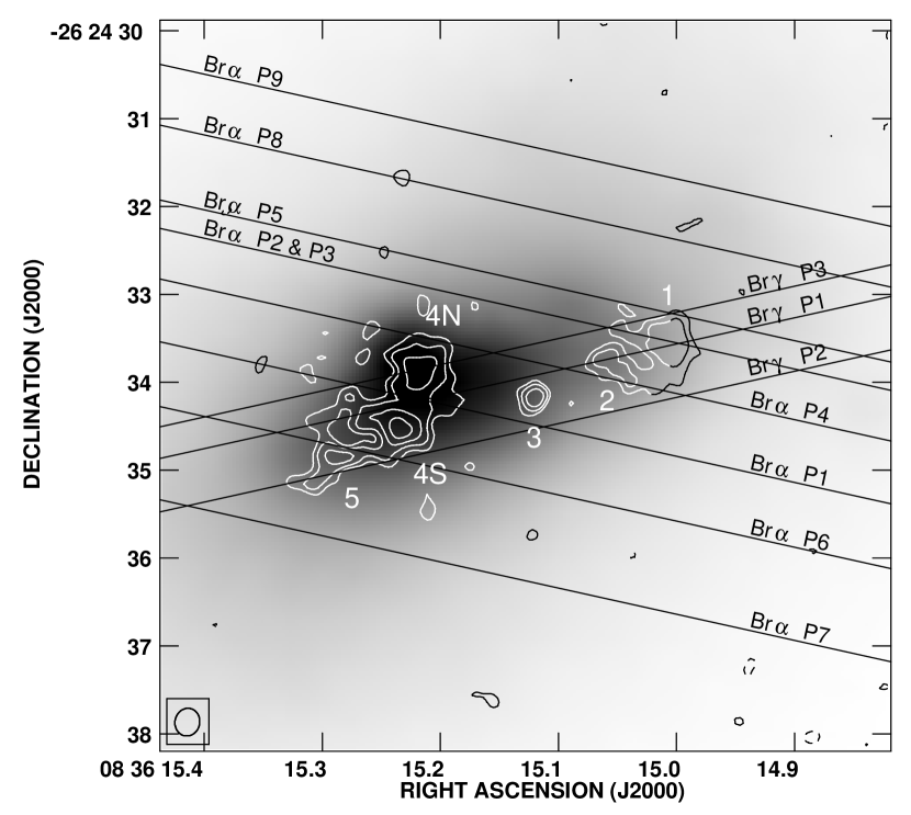
Figure 1: A VLA 1.3 cm map (contours), overlaid on an infrared SCAM image (grey scale) of He 2-10, with locations of the Brackett line slits. The coordinates of the SCAM are accurate to $\sim 0.3\arcsec$, while the VLA coordinates are accurate to $\lesssim 0.05$″. The 1.3 cm contours are 3$\sigma\times\pm 2^{n/2}$, with n = 0, 1, 2, 3 ($\sigma=40~{}\mu$Jy beam^-1 ). The beam has a FWHM of $0.32\times 0.28"$ , and a p.a. of -12°. Lines mark slit positions of the NIRSPEC Br$\gamma$ and Br$\alpha$ observations. The slits are 0″.6 wide in Br$\alpha$ and 0″.4 wide in Br$\gamma$. For most of the spectral observations, the seeing was larger than the width of the slit. We detect no spectral line emission from the positions Br$\alpha$ P7 and P9. K-band continuum is detected in the Br$\gamma$ spectra of the eastern H ii complex.

In Figure 1 we show the central region of an infrared image made by coadding the SCAM images from the night of February 10, 2003, with the slit positions superimposed. He 2-10 was imaged on the SCAM detector in both the on-target and off-target spectra. The images were sky-subtracted, and the dark pixels at the location of the slit were added to the bad pixel mask. No flat field was taken, and no photometric calibration was done. The SCAM detector is effective between 0.95 and 2.5 µm, and therefore this infrared image, which was behind the KL filter, has a bandpass of approximately 2.16 - 2.5 µm. On both nights, the seeing was $\sim 1\arcsec$ and variable, as measured from the point spread function (PSF) of the few stars in SCAM images.

We were able to determine accurate coordinates for the SCAM image in two steps. First, we created an infrared image which covered enough sky to include a few stars from the Two Micron All Sky Survey (2MASS) by mosaicking SCAM images from both on-target and off-target spectra. The resulting coordinates were accurate to $\sim 1\arcsec$, which is a rather large angular scale compared to the structure in the 1.3 cm map. We then rotated the SCAM image so that north is up and east is to the left, and shifted our coordinate solution by less than 1″, to align the peak of our SCAM emission with the coordinates of the K-band peak from Cabanac et al. (2005), which is accurate to $\pm 0.3\arcsec$. Provided the SCAM coordinates, the slit positions are easily registered with the radio emission (see Figure 1).

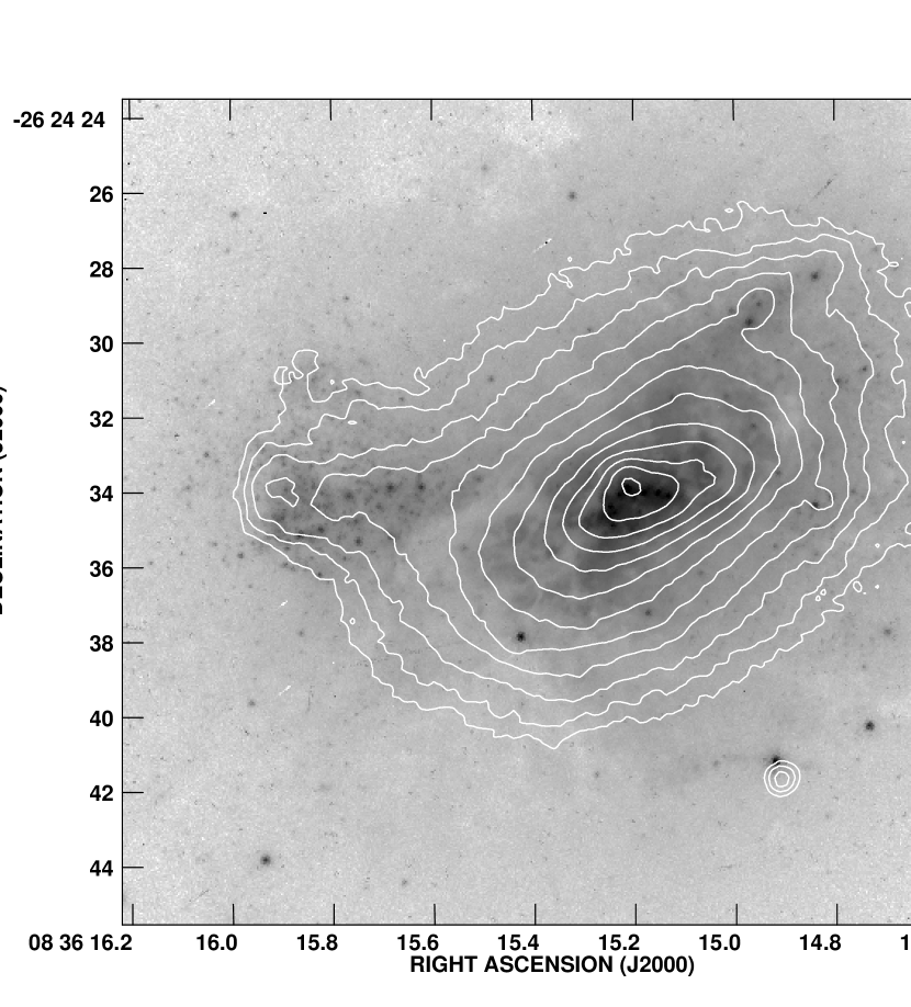
Figure 2: An F555W image of He 2-10 (grey scale), with SCAM broad band 2 µm contours. The contours are $10\sigma\times 2^{n/2}$. The extended emission to the east is the optical region B from Corbin et al. (1993), and the brighter region to the west is region A. The radio emission in Figure 1 is within the western region.

In Figure 2 we show contours of the SCAM emission, in comparison to an F555W image taken with the Wide Field Planetary Camera (WFPC2) on the Hubble Space Telescope (HST). Since coordinates taken from HST are accurate to only 1″, we take the astrometric solution from Cabanac et al. (2005), which aligns the peak of the near infrared image with the brightest optical source. The extended emission to the east is optical region B (Corbin et al., 1993), while the brighter region to the west is region A, where the more active star formation–as reflected by infrared, radio, and nebular line emission– is underway.

The high resolution spectra were spatially rectified, and a wavelength solution was applied using the NIRSPEC reduction package, REDSPEC. Arc lamp wavelength solutions obtained following these procedures are generally accurate to $\sim 1~{}{\rm km~{}s}^{-1}$ (Prato et al., 2002). In the raw L band data, we see strong, regularly spaced emission lines, which we attribute to ice on the window of NIRSPEC. Fortunately, these lines are removed by subtracting an image taken in an adjacent piece of sky. Wavelength calibration was done using lamps. Conditions were unphotometric, and we were unable to estimate slit losses due to variable seeing.

2.2 VLA Observations & Calibration

Archival VLA data, taken in the AB configuration (program AK527), were used to make the 1.3 cm map in Figure 1. The data were reduced and calibrated using the Astronomical Image Processing System (AIPS). The absolute flux calibrators were 3C48 and 3C286, and the phase calibrator was 0836-202. The measured flux of the phase calibrator was 2.3 Jy, which is within the uncertainties of Johnson & Kobulnicky (2003) in their original analysis of the data. The rms in this map is 40 $\mu$Jy beam^-1, and the FWHM of the beam is $0.32\times 0.28\arcsec$, with a position angle of -12°. We achieve a higher resolution than Johnson & Kobulnicky (2003) since their objective was to match the beam to longer wavelength observations.

The clean 1.3 cm map is shown in Figure 1. We see the sources organized in eastern and western “clumps”, as well as a central point source. There are six knots detected at 5 to 10$\sigma$, and they are labeled, following the identifications in Johnson & Kobulnicky (2003). Source 3 is the central point source, and source 4 we resolve into two sources, a northern and a southern source, which we call sources 4N and 4S.

In Table 1 we present the flux density of each knot, which we measured using AIPS. The task TVSTAT integrates the flux inside any specified region, and is ideal to measure the flux densities of crowded, extended sources, where confusion is an issue. Uncertainties are estimated from multiple attempts to measure the flux density of each knot with TVSTAT, and are $\sim 10-20$%. This uncertainty arises mostly from extended emission, which can be difficult to account for. At 1.3 cm, absolute fluxes measured with the VLA are accurate to $\sim 5$%. The flux densities which we list in Table 1 are larger than those found by Johnson & Kobulnicky (2003) because we include more extended emission.

3 Results

3.1 Brackett Line Emission

In Figures 3 and 4 our two dimensional Br$\gamma$ and Br$\alpha$ spectra show two “clumps” of emission, separated by approximately 3 - 4″ along the slit with an obvious velocity offset. Although we do not to expect to detect Brackett line emission from radio continuum source 3, which is non-thermal (Johnson & Kobulnicky, 2003), we cannot provide an upper limit because the seeing prevented us from resolving source 3 from the eastern and western complexes. K-band continuum emission is detected in the Br$\gamma$ eastern sources, but not the western sources. It is strongest in P1, but is apparent in all three spectra. This is consistent with the SCAM images (see Fig 1). There is no continuum emission detected at 4 µm.

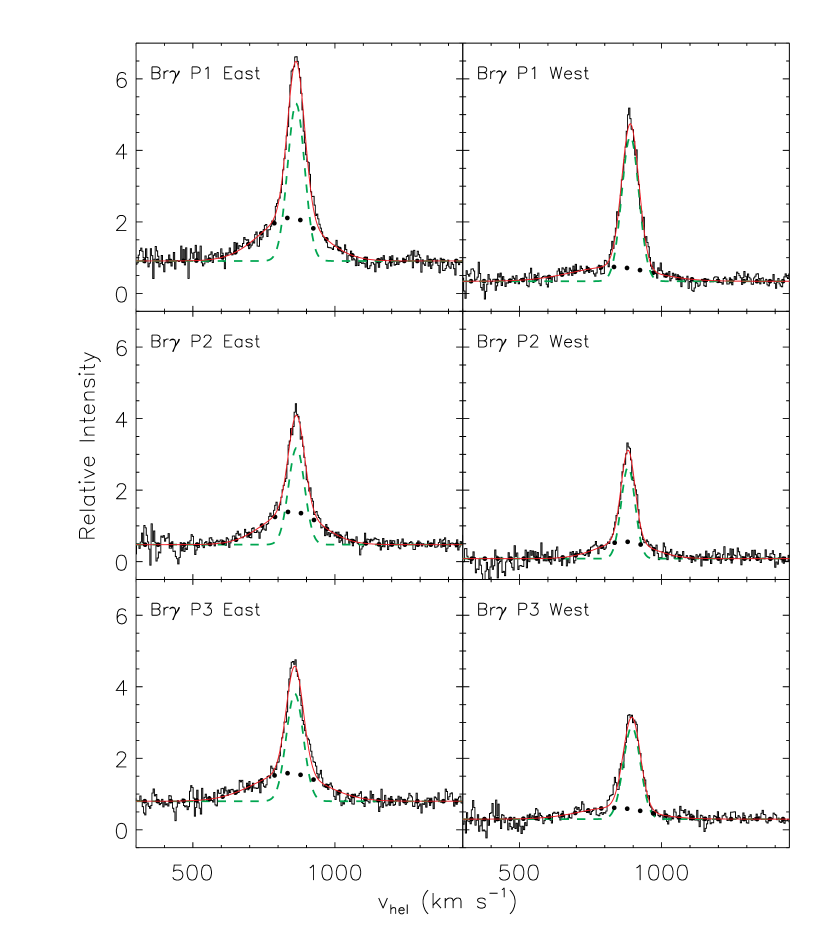
Figure 5: Br$\gamma$ 1-D Spectra. These spectra are made by integrating over 1.4″  along the slit, centered on the peaks of emission which are present in Figure 3. The red curve shows our two component Gaussian fit to the spectral lines. The dashed green curve is the narrow component of the fit, and the dotted curve represents the broad component.

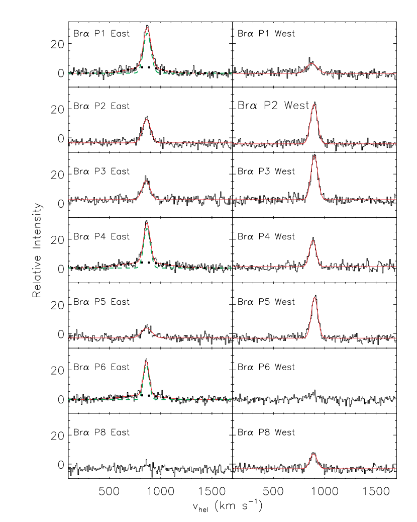
Figure 6: Br$\alpha$ one dimensional spectra. These spectra are made by integrating over 1.4″  along the slit, centered on the peaks of emission which are present in Figure 4. The red curve shows our Gaussian fit to the spectral lines. In some cases we fit two component Gaussians, which are shown as green dashed curves (narrow) and dotted curves (broad). For these spectral lines, the red curve is the sum of the two components.

In Figures 5 and 6 we show the Br$\gamma$ and Br$\alpha$ spectra, obtained by summing over a 1.4″ area along the slit, centered on the peaks of the eastern and western regions. Since the seeing was 1-1.4” over the observations, little or no spatial information was lost. In the Br$\gamma$ lines, the signal to noise is high enough to distinguish a broad, low intensity blue line wing. To quantify this component, we fit all of the Br$\gamma$ spectral lines with the superposition of two Gaussian curves, as shown in Figure 5. Line centroids and FWHM velocities of the line profiles, as well as the characterizations of the broad and narrow components, are listed in Table 2. The average velocity of the eastern sources is 862 km s^-1, while the average western velocity is 889 km s^-1, giving an average offset of 27 km s^-1 between the two regions. For comparison, Mohan et al. (2001) find $v_{hel}=873~{}{\rm km~{}s}^{-1}$ from their H92$\alpha$ radio recombination line observations, which, at a resolution of $190\times 220$ pc, average over the structure that we resolve spatially with NIRSPEC.

In addition to line profile observations, we consider relative photometry of eastern and western sources, using the Br$\gamma$ P1 spectrum where the slit went approximately through the center of each region. We find that, of the total flux in this echellogram, $\sim$ 35% is in the western sources, and $\sim$ 65% is in the eastern sources. This, agrees well with the relative fluxes in the radio, as well as at 11.7 µm  (Beck et al., 2001). On the other hand, Figure 1 shows less near infrared continuum emission coming from the western sources. This is noted by Cabanac et al. (2005), who find that extinction is larger near the western complex of H ii regions.

3.2 Radio continuum

In Table 1 we present our measurements from the 1.3 cm map, which we displayed in Figure 1. We measure 4.05 $\pm$ 0.36 mJy from the eastern sources, 1.94$\pm$ 0.15 mJy from the western sources, and 0.40 $\pm$ 0.08 mJy from the central source. The flux densities measured here are consistent with Johnson & Kobulnicky (2003), in their original analysis of the data. No single dish observations are available for comparison at 1.3 cm, but Kobulnicky & Johnson (1999) report a 2 cm flux density of $21\pm 1.2$ mJy and a 2 cm to 6 cm spectra l index of $-0.62\pm 0.11$ from low resolution VLA data. From this, we infer a total 1.3 cm flux density of $16.6\pm 1.2$ mJy, which indicates that some extended 1.3 cm emission is missed in the data presented here.

Much can be inferred from radio continuum measurements. First, one can determine the ionization rate from the thermal free-free emission:

$$\left({N_{Lyc}\over s^{-1}}\right)\gtrsim 9\times 10^{49}\left({T_{e}}\over{8000~{}K}\right)^{0.35}\left({\nu\over{\rm 22~{}GHz}}\right)^{0.1}\left({D\over{\rm Mpc}}\right)^{2}\left({F_{\nu}\over{\rm mJy}}\right).$$ (1)

Since He 2-10 has solar metallicity (Johansson, 1987), we use $T_{e}=8000$ K, typical of Galactic H ii regions. With the 1.3 cm flux densities which we measured, we derive $N_{Lyc}=3.0\times 10^{52}$ s^-1, and $N_{Lyc}=1.4\times 10^{52}$ s^-1, for the eastern and western regions, respectively. These estimates of the ionization rate are lower limits, since they assume that the H ii regions are optically thin and ionization bounded. Flux densities and brightness temperatures of the individual clusters are shown in Table 1.

With the exception of source 3, the clumps in the 1.3 cm map, which we show in Figure 1, appear to be extended. Assuming a single component Gaussian source, we use the AIPS task IMFIT to find the FWHM of each cluster. These sizes range from 30-40 pc for sources 1, 2, 4N and 4S. Source 5, which is significantly extended in the east-west direction, displays a major axis of 80 pc, and a minor axis of 30 pc. For comparison, the FWHM of the beam is 13 pc. These sources are obviously extended.

We also use the brightness temperature of the knots to estimate the nebular densities and some spatial information. For an optically thick H ii region which fills the beam, we expect $T_{b}=8000$ K. Johnson & Kobulnicky (2003) find that the flat spectra of the thermal sources turn over and become optically thick between 6-14 GHz, indicating that at 1.3 cm, the sources are optically thin. Here, the range of values represent the uncertainty in the turnover frequency, and not properties of the individual knots, which are similar. Correcting for optical depth, we expect $T_{b}\sim 350-2000$ K for sources that fill the beam for this range of turnover frequency. If we compare the observed $T_{b}$ of Table 1 to this predicted $T_{b}$, we obtain a beam filling fraction of 0.005 - 0.03, corresponding to sources of 0.4-1 pc in size. We infer that each radio source must contain further unresolved clumps of nebular material that do not fill the beam.

The turnover frequency of 6-14 GHz implies an emission measure, $\int n_{e}^{2}dl\sim 1-6\times 10^{8}$ cm^-6 pc. The density is not well constrained, as the turnover frequency and source sizes are both uncertain. The radio nebulae excited by clusters of young stars are usually found, when observed with the highest VLA resolution, to have sizes 1- 10 pc (Turner & Beck 2004; Tsai et al. 2006), which is consistent with the intensities seen here. If we adopt these as typical sizes $n_{e}$ ranges from $10^{3}$ to a few $\times 10^{4}$ cm^-3. Estimates of nebular mass are uncertain because the density and geometry are not known. If the sources are of order 1 pc, and the density $10^{4}$ cm^-3, the mass of the ionized gas in one spherically symmetric nebula is $\sim 1000~{}M_{\sun}$. Lower densities are possible, and multiple nebulae are more than likely, so the nebular mass associated with each radio source can be expected to lie between a few hundred and several thousand solar masses.

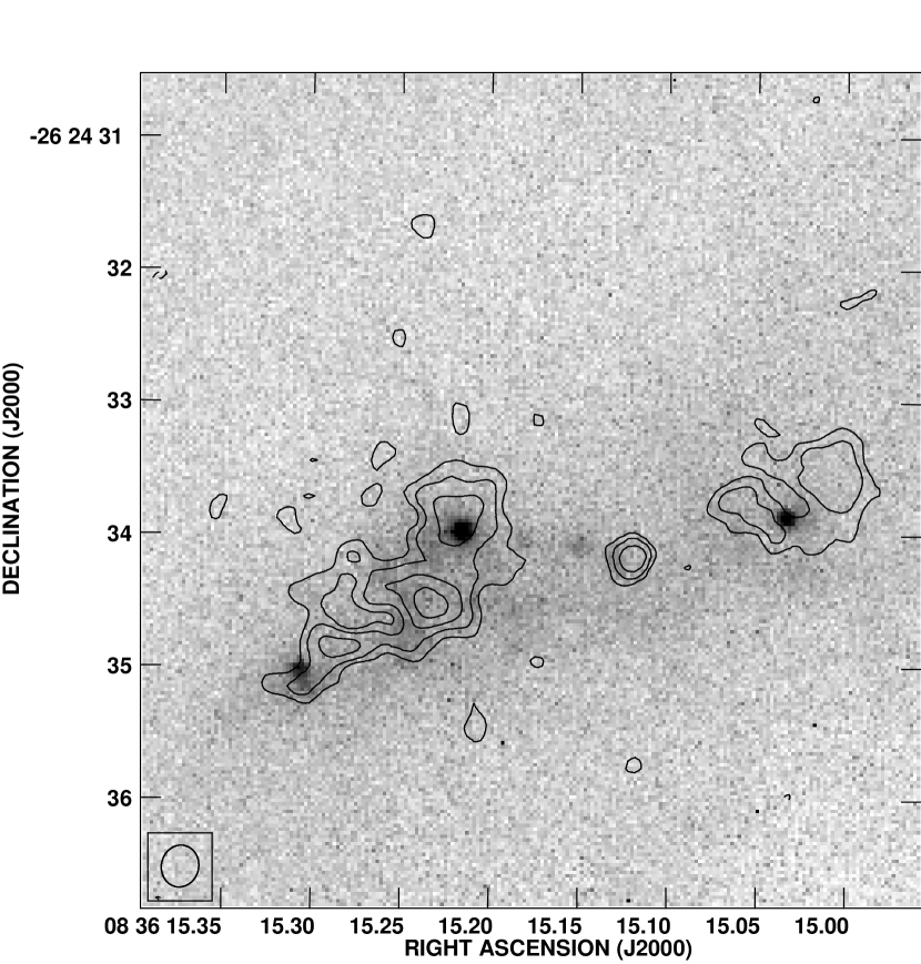
Figure 7: Grey scale: L′ image (courtesy of Cabanac et al. 2005). Contours: VLA 1.3 cm map. The contour levels are 3$\sigma~{}\times~{}\pm 2^{n/2}$, with n = 0, 1, 2, 3. The radio beam, shown in the lower left, is $0.32\times 0.28\arcsec$, with p.a. = -12°. The positional uncertainty associated with the L’ image is 0″.3, so it is uncertain which infrared sources, if any, correspond to the radio knots. In fact, there is no possible shift which will perfectly align the three brightest infrared sources with radio knots.

In Figure 7 we show an L′ map, which we received, courtesy of Cabanac et al. (2005), with our 1.3 cm contours overlaid. The positional uncertainty associated with the L′ image is 0″.3, which is still large compared to the expected size of super star clusters ($\sim$ 1 pc). Since each radio knot is likely a complex of smaller nebulae, the infrared sources could correspond to any unresolved clump or multiple thereof. As a check, we tried a variety of alignments between the 1.3 cm and the L′  image, and under no circumstances were we able to simultaneously align the three brightest infrared sources (L1, L4a, L5 from Cabanac et al. 2005) with radio knots.

4 Discussion

4.1 UV Continuum Photons

In §3.2 we calculated a total Lyman continuum rate of N${}_{Lyc}=5.3\times 10^{52}$ s^-1, from the radio continuum map, for $T_{e}=8000$ K. A number of sources have reported the ionization rate from different infrared and radio diagnostics (Mohan et al. 2001; Beck et al. 2001; Johnson et al. 2000; Kobulnicky & Johnson 1999; Johnson & Kobulnicky 2003), and a range of values have been derived. Before we attempt to determine the O star content in He 2-10, we must first account for the different estimates of N_Lyc. Here, we compare measurements which have been made in the infrared or radio, where the effects of extinction are negligible, and the light from the youngest, embedded sources can escape.

We begin by considering the Brackett line fluxes, which were reported by Kawara et al. (1989), F${}_{Br\alpha}=2.6\times 10^{-16}$ W m^-2, and F${}_{Br\gamma}=4.4\times 10^{-17}$ W m^-2. Ho et al. (1990) summarized the usage of Brackett lines as in indicator of star formation, and provide tables of the intrinsic Brackett line intensity ratio, as well as the ratio of N_Lyc/N_Brα, based on the tables of Brocklehurst (1971), Giles (1977), and Hummer & Storey (1987). From the fluxes of Kawara et al. (1989), we obtain N${}_{Lyc}=5.7\times 10^{52}$ s^-1 assuming no extinction is present at Br$\alpha$. However, we can correct for extinction at Br$\alpha$ using the differential extinction between Br$\alpha$ and Br$\gamma$. We use a $\lambda^{-\beta}$ emission law, with $\beta=1.5$, which gives A${}_{\alpha}=0.48$, and $A_{\gamma}=1.2$. With extinction correction, we get N${}_{Lyc}=6.9\times 10^{52}$ s^-1.

Other radio continuum measurements have been made by Beck et al. (2001), Kobulnicky & Johnson (1999), and Johnson & Kobulnicky (2003). From 2 cm VLA data, Kobulnicky & Johnson (1999) measured a total N${}_{Lyc}=3.5\times 10^{52}$ s^-1 by fitting Gaussian sources to the compact cores. From the same data, Beck et al. (2001) found a total $N_{Lyc}=7.3\times 10^{52}$ s^-1, by including the extended emission as well as the compact sources.

In Table 3 we summarize these results. We find that the 2 cm measurement of Beck et al. (2001) agrees with our estimate from the extinction corrected Br$\alpha$ luminosity. This suggests that the 1.3 cm measurements presented in this paper, and the 7 mm measurements of Johnson & Kobulnicky (2003) have resolved out some of the thermal emission. Considering the previous measurements, we estimate $N_{Lyc}\gtrsim 7\times 10^{52}s^{-1}$. This means that the total ionizing stellar content is equivalent to $\gtrsim$ 7000 O7 stars, where one O7 star produces 10⁴⁹ photons s^-1.

4.1.1 Cluster Masses & Luminosities

We next use the population synthesis models of Leitherer et al. (1999) to estimate the stellar mass and luminosity from the ionization rate. While the age of the starburst is generally important, the Lyman continuum rate is insensitive to age until the O stars evolved off of the main sequence and the first supernovae occur. For an upper mass cutoff of $35~{}M_{\sun}$ (Beck et al., 1997), this does not happen until an age of about 7 - 8 Myrs (Leitherer et al., 1999). The clusters appear to be younger than this, so for estimating mass, we assume that they are at the Zero Age Main Sequence (ZAMS) stage. We also assume a solar metallicity, and a Salpeter initial mass function (IMF) ($\alpha=-2.35$), with a lower mass cutoff of 1 $M_{\sun}$. We find that a luminosity of $3\times 10^{9}L_{\sun}$, and total stellar mass of at least $6\times 10^{6}~{}M_{\sun}$ will explain the inferred Lyman continuum rate for the entire starburst. If the IMF extends down to $0.1~{}M_{\sun}$, then the stellar mass will be more than twice as large. This mass agrees well with the value derived by Beck et al. (1997), using different models, but also using the Brackett line fluxes of Kawara et al. (1989). On the other hand, our derived mass is approximately six times larger than the mass determined in Johnson & Kobulnicky (2003), due to their choice of an upper mass cutoff of 100 $M_{\sun}$. This is an indication of the uncertainty in mass estimated from $N_{Lyc}$ using different IMFs. In Table 1, we list the individual source masses, which range from $\sim 1-2\times 10^{6}~{}M_{\sun}$.

4.2 Kinematics

4.2.1 The Dynamical Center: Star Formation in a disk?

How do the velocities we observed with NIRSPEC, which measure the motions of the H ii regions of the starburst, relate to the kinematics of the galaxy? The kinematics of He 2-10 are complex: it is an advanced merger, with a tidal tail extending to the southeast (Kobulnicky et al. 1995; Meier et al. 2001), and extensive dust lanes which can frustrate attempts at optical identification of structure. Kobulnicky et al. (1995) mapped the galaxy in CO and H i  and they find that the CO may be filling a hole in the H i distribution, much like large spiral galaxies with nuclear condensations of molecular gas (Scoville et al. 1989; Morris & Lo 1978). Since the H ii regions are roughly coincident with the CO emission, they are likely within the H i hole.

In addition, the H i observations show rotation with a systemic velocity of $873\pm 20~{}{\rm km~{}s}^{-1}$ (heliocentric). The central CO emission also displays a sense of rotation which is consistent with the larger scale H i emission, even though the CO has an asymmetric, tidal tail appearance. We find velocity centroids of $890\pm 10~{}{\rm km~{}s}^{-1}$ for the western H ii regions, and $862\pm 5~{}{\rm km~{}s}^{-1}$ for the eastern H ii regions. We compare these velocities to the CO channel maps in Kobulnicky et al. (1995), and find that the western H ii regions are approximately coincident with the peak of the CO in their $896~{}{\rm km~{}s}^{-1}$ channel, and the eastern H ii regions are close to the peak of the CO emission in their $865~{}{\rm km~{}s}^{-1}$ channel. This is consistent with the H ii regions moving at the velocities of the molecular clouds from which they were born.

4.2.2 Line Profiles: Width

We present the measured line widths of all the lines in Table 1. The FWHM are consistently 60-80 km s^-1. The widths of hydrogen recombination lines from a H ii regions will include the effects of thermal broadening, electron impact broadening, and broadening due to different velocities in the gas (added in quadrature). Thermal broadening at $T_{e}$ of 8000 K is $\sim$ 20 km s^-1 (FWHM), and electron impacts have a negligible effect at the low quantum numbers of Brackett lines. So the non-thermal width of the lines, that is the width due to gas motions, is $\sim$57 to 77 km s^-1.

Are the recombination lines in He 2-10 wide because at 9 Mpc, the beam encompasses more sources than in Galactic surveys? We can estimate the contribution to the gas motions of the velocity dispersion of the multiple sources in the beam. Based on the estimated masses of the star clusters within the nebulae (§4.1) of 4 and $2\times 10^{6}~{}M_{\sun}$, and for the observed sizes of 50-70 pc, we would predict Brackett linewidths of $15-20~{}{\rm km~{}s}^{-1}$ for both the eastern and western complexes. Since the contributions of the gas motions and the thermal line width add in quadrature, there must remain a component of 51-75 km s^-1 in the line widths which must be due to turbulence, outflow, or some other velocity field in the gas.

The observed line widths are highly supersonic, but not at all unusual for dense, young star formation regions. Garay & Lizano (1999) tabulate the widths of recombination lines from Galactic compact H ii regions and find that while most have FWHM between 30 and 50 km s^-1, many have FWHM as high as 80 km s^-1. However, these Galactic H ii regions are excited by single stars and do not have the velocity dispersion contribution of the clusters in He 2-10. These core line widths for H ii regions with luminosity $\sim 10^{9}L_{\sun}$, are similar to those of Galactic regions with luminosity $\sim 10^{5}L_{\sun}$ (Turner et al., 2003).

If each of our radio knots is treated as a single nebula, expanding at 30-40 km s^-1 to its current size, they would be $3-7\times 10^{5}$ years old. But Galactic Compact H ii regions under the same analysis would be only a few thousand years old: those dynamical arguments greatly underestimate the age of H ii regions (Dreher & Welch 1981; Wood & Churchwell 1989).

Because the individual clusters within each radio knot are unresolved we cannot calculate the escape velocities. But given the large stellar masses, and the small radii observed for other sources, such as the one in the dwarf galaxy NGC 5253 (Turner et al., 2003) it is possible that for at least some of the sub-sources the escape velocities are comparable to the supersonic gas velocities observed. If this is so, then gravity will play an important role in the evolution of these nebulae and, unlike the case in typical Galactic H ii regions, cannot be neglected.

4.2.3 Line Profiles: High Velocity, Blue Wings

In Figure 5, one of the most obvious spectral line features is the asymmetric, blue line wing, which is most obvious in the Br$\gamma$ P1 spectrum. This feature is also seen in H$\alpha$ line profiles (Kawara et al. 1987; Méndez & Esteban 1997). A single Gaussian profile is inadequate at describing the line profile, so we fit the line with the superposition of two Gaussian curves, as described in §3.1. The broad, low intensity component is shifted approximately 20 km s^-1 blue of the central peak. For comparison, we fit similar profiles to some of the Br$\alpha$ spectra in Figure 6, where a similar blue line wing is detected at $\sim 1.5-2.0\sigma$. We list the parameters of these fits in Table 2. For Br$\gamma$, the FWHM of the broad component is 200-300 km s^-1, which is consistent with H$\alpha$ profiles presented by Kawara et al. (1987).

We consider possible explanations for the high velocity gas motions. First, He 2-10 contains several optical clusters which display WR features (Chandar et al., 2003), and do not have strong Brackett-emitting counterparts. There are also large scale bubbles present in H$\alpha$ narrow band images, and similar high velocity motions are present in H$\alpha$ lines, out to distances of $\sim$ 500 pc from the starburst (Méndez & Esteban 1997; Méndez et al. 1999). One possibility, is that one or several of the centrally located, more evolved optical clusters is driving high velocity gas motions. In this model, stellar winds impinge on nearby, Brackett-emitting H ii regions, causing the high velocity motion which we see. We note that the broad component is stronger in the eastern regions than the western regions, as seen in Figures 5 and 6. This could be the result of higher extinction in the western regions, or there may simply be more high velocity gas in the east.

Alternatively, the embedded, young stars within the Brackett line emitting regions could be the source of high velocity motions. Bouret et al. (2005) and Puls et al. (1996) have modeled H$\alpha$ line profiles of O star winds in the Galaxy, and for sources where the P-Cygni absorption is minimal or non- existent, they exhibit similar, asymmetric line profiles. In these sources internal obscuration suppresses the red wing of the line, causing asymmetry. Kawara et al. (1989) suggest an average of 1-2 magnitudes of extinction in the K-band, so this is not unreasonable. In a stellar wind, we expect this effect of extinction to be less pronounced in Br$\alpha$, resulting in a broad component which is wider, and redshifted relative to that in Br$\gamma$. Where the broad component is detected, it has a FWHM of 300-500 km s^-1, significantly wider than the broad Br$\gamma$ components. However, we can not determine if the centroid of the broad Br$\alpha$ component is shifted because of the low S/N in the wing of the Br$\alpha$ line and the differences in the slit orientation between Br$\alpha$ and Br$\gamma$.

In actuality, we are observing H ii regions rather than stellar winds, and complex kinematics are a reality. H ii regions have a variety of morphologies, including champagne flows, shells, or cometary structure (see Garay & Lizano 1999). It is possible that higher velocity gas is more deeply embedded in the nebulae, and that Br$\alpha$ is mapping different kinematics than the Br$\gamma$. This could explain the larger velocities in the broad component of Br$\alpha$, without requiring a redshift relative to Br$\gamma$.

5 Conclusions

The dwarf galaxy He 2-10 contains an intense starburst, which is resolved into two major complexes of H ii regions, separated by approximately 150 pc. What has triggered the starburst, and why are there two complexes of H ii regions? Is there anything we can infer about the evolution of the starburst? The high extinction and dense gas in the H ii regions indicate that these star-forming regions are young. The H ii regions are both spatially and kinematically coincident with the CO emission (§4.2). Whether the fundamental cause of the starburst is a merger or accretion of interstellar gas, the immediate cause is a concentration of molecular gas near the center of the galaxy.

We have analyzed high spectral resolution Brackett line spectra of the two H ii complexes in Henize 2-10. The Brackett line profiles provide substantial kinematic information about the star clusters and associated nebulae. The line profiles, particularly Br$\gamma$ where the S/N is high, show a broad blue wing. The line profile can be fit by a two component Gaussian, where one component is broad, low intensity, and blue shifted relative to a more narrowly peaked line center. This line profile can be explained by extinction internal to the nebulae, which is suppressing the emission from gas that would otherwise appear redshifted. This high velocity gas motion, taken with the clumpy nature of the sources, suggests that the young star clusters in He 2-10 may be in the process of dispersing their nebular material via winds.

The two complexes of H ii regions appear to be associated with two kinematically distinct molecular clouds. We find an obvious velocity offset between our eastern and western H ii regions. Comparison to the CO channel maps of Kobulnicky et al. (1995) suggests that the Brackett line centroids are consistent with the velocities of the molecular gas from which these clusters formed.

We also use archival VLA observations of the H ii regions to estimate stellar mass, as well as the sizes and nebular densities of the H ii regions. We find that each thermal radio source contains $1-2\times 10^{6}~{}M_{\sun}$. The 1.3 cm maps also indicate that the mass and nebular material are not distributed in a single cluster and nebula. There are most likely multiple clumps of star formation associated with each radio knot. That the H ii regions appear in the radio continuum and are not extremely optically thick suggests that they are somewhat evolved and beginning to expand and disperse.

The line profiles we see in He 2-10 present the same paradoxes seen in NGC 5253 and other galaxies (Turner et al. 2001; Turner et al. 2003). The He 2-10 clusters contain many O stars, each of which may be presumed to drive a wind with velocity on the order of 1000 km s^-1. Yet the narrow core of the He 2-10 lines (FWHM) is no wider than that of many Galactic H ii regions with one O star. Unlike the NGC 5253 source, the He 2-10 lines have weak but broad wings. This shows a body of fast moving gas that may soon break out of the original cluster environment, while much of the line luminosity is confined.

The picture of He 2-10 presented by these kinematical considerations is a snapshot of an aging starburst, in which the neutral gas is beginning to settle into patterns typical of spiral galaxies, with centrally concentrated molecular gas, and an H i ring. The starburst is aging, and the winds of the young stars are becoming prominent in the ionized gas, reflected in blue-shifted flows of FWHM 200-300 km s^-1. Discovering the origins of the starburst amid these intense evolutionary forces will be challenging.

Figure 3: Br$\gamma$ two dimensional spectra. Up is to the southeast, with the top (bottom) peak of emission representing the eastern (western) nebulae. Contour levels are 3$\sigma\times\pm 2^{n/2}$, n =0, 1, 2, 3, 4, with $\sigma\approx.06$ counts pixel^-1. The eastern spectra also display contiuum emission.

Figure 4: Br$\alpha$ two dimensional spectra. Up is to the northeast, with the top (bottom) peak of emission representing the eastern (western) nebulae. Contour levels are 3$\sigma\times\pm~{}2^{n/2}$, n = 0, 1, 2, 3, 4, with $\sigma\approx 0.6$ counts pixel^-1. No continuum sources are detected at any location.

Table 1: Radio Knot Properties

Source	$\alpha$	$\delta$	$F_{1.3cm}$	$T_{B}$	O7 stars	Mass
	(J2000)	(J2000)	(mJy)	(K)		($10^{6}M_{\sun}$)
1	8 36 15.000	-26 24 33.600	1.08 $\pm$ 0.11	7.0	1900	1.3
2	8 36 15.062	-26 24 33.720	0.86 $\pm$ 0.10	6.4	1100	0.7
3	8 36 15.122	-26 24 34.185	0.40 $\pm$ 0.08	10.0	$\cdots$	$\cdots$
4N	8 36 15.218	-26 24 33.905	1.61 $\pm$ 0.25	9.4	2300	1.5
4S	8 36 15.235	-26 24 34.960	1.52 $\pm$ 0.24	12	2500	1.7
5	8 36 15.286	-26 24 34.840	0.92 $\pm$ 0.10	8.5	1200	0.8

Table 2: Brackett Line Profiles

	Eastern Region								Western Region
	Total		Narrow		Broad		F${}_{narrow}/F_{broad}$		Total		Narrow		Broad		F${}_{narrow}/F_{broad}$
Spectrum	$v$	FWHM	$v$	FWHM	$v$	FWHM			$v$	FWHM	$v$	FWHM	$v$	FWHM
	(km s-1)								(km s-1)
Br$\gamma$
P1	861$\pm 1$	66$\pm 2$	863$\pm 1$	70$\pm 3$	843 $\pm 3$	254$\pm 10$	1.0$\pm 0.1$		887$\pm 1$	61$\pm 2$	890$\pm 1$	71$\pm 1$	824$\pm 11$	331$\pm 24$	2.2$\pm 0.2$
P2	860$\pm 1$	62$\pm 2$	865$\pm 1$	67$\pm 2$	849$\pm 4$	237$\pm 13$	0.8$\pm 0.1$		880$\pm 1$	57$\pm 2$	882$\pm 1$	57$\pm 2$	869$\pm 7$	223$\pm 21$	1.4$\pm 0.1$
P3	857$\pm 1$	58$\pm 2$	859$\pm 1$	71$\pm 2$	837$\pm 5$	287$\pm 14$	0.9$\pm 0.1$		891$\pm 1$	59$\pm 2$	895$\pm 1$	71$\pm 2$	829$\pm 14$	284$\pm 28$	2.0$\pm 0.2$
Br $\alpha$
P1	867$\pm 1$	85$\pm 4$	869$\pm 1$	85$\pm 2$	847$\pm 11$	37$\pm 39$	1.5$\pm 0.2$		872$\pm 1$	64$\pm 10$	$\cdots$	$\cdots$	$\cdots$	$\cdots$	$\cdots$
P2	862$\pm 1$	80$\pm 10$	$\cdots$	$\cdots$	$\cdots$	$\cdots$	$\cdots$		895$\pm 1$	78$\pm 9$	$\cdots$	$\cdots$	$\cdots$	$\cdots$	$\cdots$
P3	859$\pm 1$	59$\pm 8$	$\cdots$	$\cdots$	$\cdots$	$\cdots$	$\cdots$		899$\pm 1$	72$\pm 8$	$\cdots$	$\cdots$	$\cdots$	$\cdots$	$\cdots$
P4	866$\pm 1$	72$\pm 5$	866$\pm 1$	76$\pm 2$	835$\pm 14$	528$\pm 62$	1.0$\pm 0.1$		884$\pm 1$	65$\pm 4$	$\cdots$	$\cdots$	$\cdots$	$\cdots$	$\cdots$
P5	863$\pm 1$	74$\pm 10$	$\cdots$	$\cdots$	$\cdots$	$\cdots$	$\cdots$		901$\pm 1$	69$\pm 6$	$\cdots$	$\cdots$	$\cdots$	$\cdots$	$\cdots$
P6	859$\pm 1$	64$\pm 6$	860$\pm 1$	63$\pm 2$	805$\pm 15$	432$\pm 53$	1.2$\pm 0.2$		$\cdots$	$\cdots$	$\cdots$	$\cdots$	$\cdots$	$\cdots$	$\cdots$
P8	$\cdots$	$\cdots$	$\cdots$	$\cdots$	$\cdots$	$\cdots$	$\cdots$		890$\pm 1$	74$\pm 7$	$\cdots$	$\cdots$	$\cdots$	$\cdots$	$\cdots$

Note. — Velocities are heliocentric. Values are given for the total emission line, as well as the narrow and broad Gaussian components.

Table 3: UV continuum measurements

$N_{Lyc}$ (1052 s-1)	Authors	Technique
$\gtrsim$ 2.5	Mohan et al. (2001)	radio recombination line models
5.7	Kawara et al. (1989)	Br$\alpha$, no extinction correction
6.9	Kawara et al. (1989)	Br$\alpha$, extinction corrected
5.1	Johnson & Kobulnicky (2003)	7 mm continuum flux
4.4	this paper	1.3 cm continuum flux
11.8	Beck et al. (2001)	Dust heating
3.5	Kobulnicky & Johnson (1999)	2 cm continuum flux, compact cores only
7.3	Beck et al. (2001)	2 cm continuum flux, compact cores plus extended emission

References

- Allen et al. (1976) Allen, D. A., Wright, A. E., & Goss, W. M. 1976, MNRAS, 177, 91
- Beck et al. (1997) Beck, S. C., Kelly, D. M., & Lacy, J. H. 1997, AJ, 114, 585
- Beck & Kovo (1999) Beck, S. C. & Kovo, O. 1999, AJ, 117, 190
- Beck et al. (2001) Beck, S. C., Turner, J. L., Gorjian, V. 2001, AJ, 122, 1365
- Beck et al. (2002) Beck, S. C., Turner, J. L., Langland-Shula, L. E., Meier, D. S., Crosthwaite, L. P., & Gorjian, V. 2002, AJ, 124, 2516
- Bouret et al. (2005) Bouret, J.-C., Lanz, T., & Hillier, D. J. 2005, A&A, 438, 301
- Brocklehurst (1971) Brocklehurst, M. 1971, MNRAS, 153, 471
- Cabanac et al. (2005) Cabanac, R. A., Vanzi, L., & Sauvage, M. 2005, ApJ, 631, 252
- Chandar et al. (2003) Chandar, R., Leitherer, C., Tremonti, C., & Calzetti, D. 2003, ApJ, 586, 939
- Corbin et al. (1993) Corbin, M. R., Korista, K. T., Vacca, W. D., 1993, AJ, 105, 1313
- Davies et al. (1998) Davies, R. I., Sugai, H., & Ward, M. J. 1998, MNRAS, 295, 43
- Dreher & Welch (1981) Dreher, J. W., & Welch, W. J. 1981, ApJ 245, 857
- Garay & Lizano (1999) Garay, G., & Lizano, S. 1999, PASP, 111, 1049
- Giles (1977) Giles, K. 1977, MNRAS, 180,578
- Ho et al. (1990) Ho, P. T. P., Beck, S. C., & Turner, J. L. 1990, ApJ, 349, 57
- Hummer & Storey (1987) Hummer, D. G., & Storey, P. J., 1987, MNRAS, 224, 801
- Johansson (1987) Johansson, L. 1987, A&A, 182, 179
- Johnson & Kobulnicky (2003) Johnson, K. J., Kobulnicky, H. A. 2003, ApJ, 597, 923
- Johnson et al. (2000) Johnson, K. J., Leitherer, C., Vacca, W. D., & Conti, P. S. 2000, AJ, 120, 1273
- Kawara et al. (1989) Kawara, K., Nishida, M., & Phillips, M. M. 1989, ApJ, 337, 230
- Kawara et al. (1987) Kawara, K., Taniguchi, Y., Nishida, M. &, Jugaku, J. 1987, PASP, 99, 512
- Kobulnicky et al. (1995) Kobulnicky, H. A., Dickey, J. M., Sargent, A. I., Hogg, D. E., Conti, P. S. 1995, AJ, 1995, 110, 116
- Kobulnicky & Johnson (1999) Kobulnicky, H. A., & Johnson, K. E. 1999, ApJ, 527, 154
- Leitherer et al. (1999) Leitherer, C., Schaerer, D., Goldader, J. D., Delgado, R., Robert, C., Kune, D. F., De Mello, D. F., Devost, D., Heckman, T. M. 1999, ApJS, 123, 3
- McLean et al. (1998) McLean, I. S., et al. 1998, Proc. SPIE, 3354, 566
- McLean et al. (2000) McLean, I. S., Graham, J. R., Becklin, E. E., Figer, D. F., Larkin, J. E., Levenson, N. A., & Teplitz, H. I. 2000, Proc. SPIE, 4008, 1048
- Meier et al. (2001) Meier, D. S., Turner, J. L., Crosthwaite, L. P., Beck, S. C. 2001, AJ, 121, 740
- Méndez & Esteban (1997) Méndez, D. I., & Esteban, C. 1997, ApJ, 488, 652
- Méndez et al. (1999) Méndez, D. I., Esteban, C., Filipovic, M. D., Ehle, M., Haberl, F., Pietsch, W., & Haynes, R. F. 1999, A&A, 349, 801
- Mohan et al. (2001) Mohan, N. R., Anantharamaiah, K. R., & Goss, W. M. 2001, ApJ, 557, 659
- Morris & Lo (1978) Morris, M., & Lo, K. Y. 1978, ApJ, 223, 803
- Ott et al. (2005) Ott, J., Walter, F., & Brinks, E. 2005, MNRAS, 358, 1423
- Prato et al. (2002) Prato, L., Simon, M., Mazeh, T., McLean, I. S., Norman, D., & Zucker, S. 2002, ApJ, 569, 863
- Puls et al. (1996) Puls, J., Kudritzki, R.-P., Herrero, A., Pauldrach, A. W. A., Haser, S. M., Lennon, D. J., Gabler, R., Voels, S. A., Vilchez, J. M., Wachter, S., Feldmeier, A. 1996, A&A, 305, 171
- Sauvage et al. (1997) Sauvage, M., Thuan, T. X., & Lagage, P. O. 1997, A&A, 325, 98
- Scoville et al. (1989) Scoville, N. Z., Sanders, D. B., Sargent, A. I., Soifer, B. T., & Tinny, C. G. 1989, ApJ, 345, L25
- Tsai et al. (2006) Tsai, C.-W., Turner, J. L., Beck, S. C., Crosthwaite, L. P., Ho, P. T. P., & Meier, D. S., 2006, AJ, in press
- Turner & Beck (2004) Turner, J. L., & Beck, S. C. 2004, ApJ, 602, L85
- Turner et al. (2000) Turner, J. L., Beck, S. C., & Ho, P. T. P. 2000, ApJ, 421, 122
- Turner et al. (2003) Turner, J. L., Beck, S. C., Crosthwaite, L. P., Larkin, J. E., McLean, I. S., & Meier, D. S. 2003, Nature, 423, 621
- Turner et al. (2001) Turner, J. L., Beck, S. C., Crosthwaite, L. P., & Meier, D. S. 2001, BAAS, 33, 1449
- Vacca & Conti (1992) Vacca, W. D., & Conti, P. S. 1992, ApJ, 401, 543
- Wood & Churchwell (1989) Wood, D. O. S., & Churchwell, E., ApJS, 69, 831