Time series photometry of the dwarf planet ERIS (2003 UB313)

Abstract

Context. The dwarf planet Eris (2003 UB313, formerly known also as “Xena”) is the largest KBO up to now discovered. Despite being larger than Pluto and bearing many similarities with it, it has not been possible insofar to detect any significant variability in its light curve, preventing the determination of its period and axial ratio.

Aims. We attempt to assess the level of variability of the Eris light curve by determining its BVRI photometry with a target accuracy of 0.03 mag/frame in R and a comparable or better stability in the calibration.

Methods. Eris has been observed between November $30^{\mathrm{th}}$ and December $5^{\mathrm{th}}$ 2005 with the Y4KCam on-board the 1.0m Yale telescope at Cerro Tololo Interamerican Observatory, Chile in photometric nights.

Results. We obtain 7 measures in B, 23 in V, 62 in R and 20 in I. Averaged B, V, and I magnitudes as colors are in agreement within $\approx 0.03$ mag with measures from Rabinowitz et al. (2006) taken in the same nights. Night-averaged magnitudes in R shows a statistically significant variability over a range of about $0.05\pm 0.01$ mag. This can not be explained by known systematics, background objects or some periodical variation with periods less than two days in the light-curve. The same applies to B, V and to less extent to I due to larger errors.

Conclusions. In analogy with Pluto and if confirmed by future observations, this “long term” variability might be ascribed to a slow rotation of Eris, with periods longer than 5 days, or to the effect of its unresolved satellite “Dysnomea” which may contribute for $\approx 0.02$ mag to the total brightness.

1 Introduction

Since its discovery the dwarf planet 2003 UB313 has attracted a lot of attention being the first Trans Neptunian Object (TNO) larger than Pluto ever discovered (Brown et al., 2005). This object, recently baptized “Eris” (IAU, 2006), revealed a number of features in common with Pluto, despite being a member of the family of the scattered TNO (Sheppard, 2006).

As an example, like Pluto Eris has a satellite named “Dysnomea” with orbital period of about two weeks, a brightness of about $2\%$ of that of Eris, a semi-major axis of $\approx 5\times 10^{4}$ Km (Brown et al., 2006a). Eris IR spectrum is clearly dominated by CH₄ absorption bands (Brown et al., 2006b) and perhaps shows $N_{2}$ bands (Licandro et al., 2006). When compared with other TNOs its colors are quite neutral and not significantly reddened (Rabinowitz et al., 2006). Its phase function at small phase angles is quite flat (Rabinowitz et al., 2006). Up to now its light curve did not reveal any trace of significant variability or periodicity (Brown et al., 2005; Rabinowitz et al., 2006). These features suggests Eris to be an icy body which is subject to frequent resurfacing likely due to evaporation and redeposition of a tiny atmosphere as its heliocentric distance changes (Brown et al., 2005; Rabinowitz et al., 2006).
In this Letter we present BVRI photometry of Eris obtained during 5 nights in late 2005 with the aim of building up a light curve and searching for possible periodicity. The same data-set is used to better constrain the optical colors of the object.

		B	V	R	I
Night	Date	[mag]	[mag]	[mag]	[mag]
1	Nov. 30, 2005	$19.619\pm 0.041$	$18.766\pm 0.025$	$18.384\pm 0.010$	$18.019\pm 0.030$
2	Dec. 1, 2005	$19.540\pm 0.038$	$18.768\pm 0.015$	$18.368\pm 0.007$	$18.029\pm 0.032$
3	Dec. 2, 2005	$19.651\pm 0.066$	$18.772\pm 0.015$	$18.388\pm 0.007$	$17.948\pm 0.022$
4	Dec. 3, 2005	$19.678\pm 0.052$	$18.788\pm 0.016$	$18.397\pm 0.007$	$17.975\pm 0.022$
5	Dec. 4, 2005	$19.616\pm 0.077$	$18.802\pm 0.015$	$18.422\pm 0.007$	$18.039\pm 0.027$

Table 1: Weighted averages of BVRI for each night.

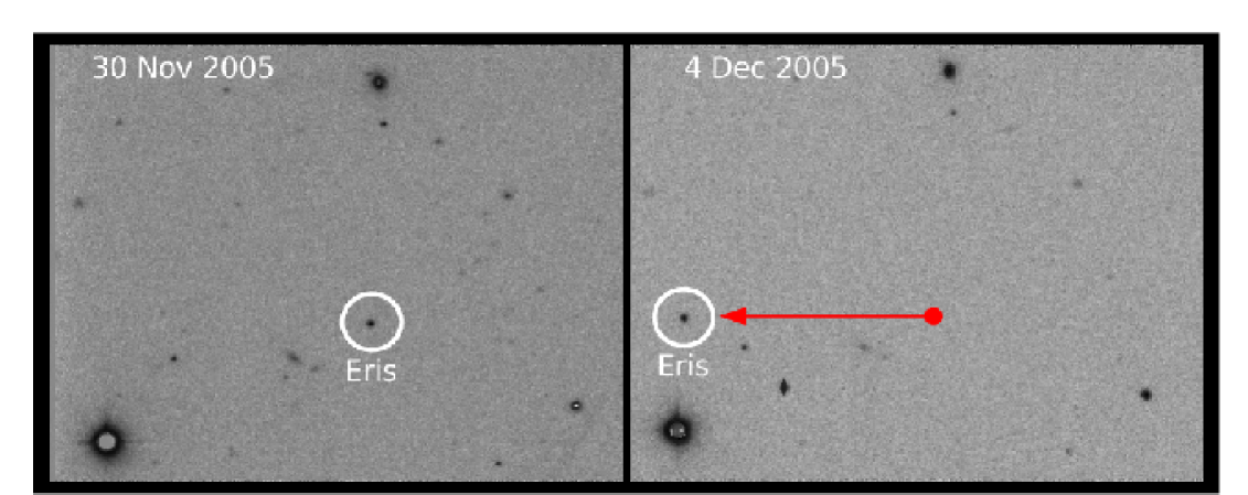
Figure 1: Eris position in the first (left panel) and last night (right panel). The area is 3.5 $\times$ 2.7 arcmin. North in down, East to the right. The arrow indicates Eris motion over the whole run.

2 Observations and Data Reduction

We observed Eris over 5 consecutive nights (November 30 to December 4, 2005). Photometric data were obtained with the Y4KCam CCD on-board the Yale 1.0m telescope at Cerro Tololo Interamerican Observatory, which is operated by the SMARTS consortium. The Y4KCam instrument is a 4096 $\times$ 4096 CCD with a pixel scale of 0.289^′′, which allows one to observe a field 20 arcmin on a side on the sky. An image of the field around Eris is shown in Fig. 1. A series of images in BVRI was acquired in order to constraint both the light curve and the colors. A total of 7 images in B, 23 in V, 62 in R and 20 in I has been obtained over the observing run, and the exposure times were 300-600 secs. The nights were all photometric but for the last one (December 4, 2005), with typical seeing ranging from 0.8 to 1.2 arcsec. The images were cleaned and pre-reduced using the pipeline developed by Phil Massey. To extract Eris magnitudes we used the QPHOT task within IRAF, which allows one to measure aperture photometry. For Eris we used a small aperture (7 pixels). Together with Eris we measured 5 field stars with roughly the same magnitude ($17.53\leq\langle R\rangle\leq 19.25$). Due to the slow motion of Eris and the wide field covered by the CCD, we could measure the same 5 stars every night and thus tie the photometry to the same zero point for the entire data-set. For the field stars we used a larger aperture (18 pixels). Absolute magnitudes were derived by shifting Eris magnitudes to the first night using the reference field stars. A set of bright stars in the first night were used to aperture-correct the magnitudes. Aperture corrections were found to be small, of the order of 0.05-0.12 mag. The zero points of the photometry was then obtained through the observation of 50 standard stars in the Landolt (1982) fields PG0231, SA92 and Rubin149, using as well a large aperture of 18 pixels. The magnitudes were also color-corrected using Eris mean colors. The final photometry, consisting of 115 data points, is reported in Tab. 2 together with the photometric error, UT time, and filter. In the same period we observed, Rabinowitz et al. (2006) have obtained 2 B, 4 V and 2 I  images of Eris. We compared our photometry with their one, and found a good agreement, being $\Delta B=0.05$, $\Delta V=-0.032$ and $\Delta I=0-0.022$, in the sense our photometry minus their one. We have not direct comparison with R, since these authors did not publish data in R for these nights.

3 Light curve and period hunting

Fig. 2 shows night-by-night time dependencies in the R band. It is evident that, even removing the four measures with anomalously large errors ($\Delta R>0.04$ mag), the dispersion of data can not be attributed just to random errors. The weighted average for all of the five nights gives $\bar{R}=18.3916\pm 0.0033$ mag with $\chi^{2}=136$ and 57 d.o.f. (degree of freedom), a $\chi^{2}$-test rejects the hypothesis of random fluctuations at a confidence level ($\mathrm{c.l.}$) $\sim 2\times 10^{-8}$ insensitive to the exclusion of the bad measures. Inspection of the R frames shows that Eris is moving very slowly in an uncrowded field (see Fig. 1), with no evident objects in background. Moreover, due to the short exposures and the low proper motion, both Eris and field stars are round without trailing. All together this seems to exclude at least the most common systematic effects. The observing conditions (heliocentric distance $r_{\mathrm{h}}$, geocentric distance $\Delta$, as phase angles $\alpha$) could be responsible for the effect. However, during the five nights they were fairly stable. In fact the object moves of about 95 arcsec in 5 nights. The change in $r_{\mathrm{h}}\Delta$ explains no more than $1.7\times 10^{-3}$ mag. On the other hand, the phase angle changes of $\Delta\alpha=0.0246^{\circ}$ during the observations. No phase coefficients in R have been published so far for Eris, but assuming as an upper limit the same phase coefficient of V in Rabinowitz et al. (2006), the phase effect would account at most for $3.5\times 10^{-3}$ mag. In conclusion, obvious changes in the observing conditions excludes geometrical effects.
Tab. 1 reports weighted averages for magnitudes taken in the same night, while the lower frame of Fig. 3 displays the same data for the R filter. A clear trend appears in R for nights 2 to 5.
A $\chi^{2}$ test rejects the hypothesis of random fluctuations at c.l. $\approx 2\times 10^{-6}$, inclusion of night 1 does not change this result. This is robust against selection of data according to the U.T. of observation (as evident from Fig. 2 in night 1 Eris has been observed just between $U.T.=2$ and $U.T.=4$ considering only data in that U.T. interval does not change the result) and replacing weighted averages with median estimation of nightly centroids. The difference between nights 5 and 2 is $0.054\pm 0.010$ mag, equivalent to $5.4\sigma$. A linear fit for nights 2 to 5 gives a slope $R^{\prime}\approx 0.0170\pm 0.0002$ mag/day with $\chi^{2}_{\mathrm{linear}}=0.99$ equivalent to c.l. $\approx 0.6$ that residual fluctuations are just due to errors. A parabolic fit including all the nights gives $\chi^{2}_{\mathrm{parabolic}}=2.35$ equivalent to a c.l. $\approx 0.3$.
The lower panel of Fig. 3 compares variations for 5 field stars having R in the approximated range $17.5$ mag - $19.3$ mag encompassing the range of Eris R magnitudes. Magnitudes are measured frame by frame and averaged over each night in the same manner of Eris data. To highlight the variations, the first night of each serie has been shifted to the averaged R for Eris, R=18.39 mag. It is evident that field stars are stable with peak-to-peak variations in R of about 0.01 mag. The only star departing from this value is the weakest in the serie having $R=19.3$ mag. In addition the expected random errors for field stars are similar to the random errors for Eris. Larger errors appearing for R larger then $19$ mag. A convincing test of the calibration stability comes from the fact that variability indicators for field stars (either peak-to-peak variation, the r.m.s. between the 4 nights, the $\chi^{2}$ for fitting against a constant value or better the related significativity) plotted as a function of their mean magnitude are constant for R up to $\approx 19$ mag. Moreover, for Eris the indicators of variability allways differ significantly from the values obtained for field stars below $R=19$ mag. Peak-to-peak variations for field stars is $\approx 0.011$ mag - $0.012$ mag v.z. Eris 0.029 mag. Night-by-night rms for the field stars is $\approx 0.005$ - $0.006$ mag, v.z. Eris 0.012 mag. The significativity of fluctuations for field stars is always below the 60% level v.z. Eris showing fluctuations with a significativity larger than 98%. In addition, field starts fluctuations are not very much correlated with Eris fluctuations, in some cases field stars are anticorrelated with Eris and correlations are not much significant. All this supports the idea that Eris brightness variations are not due to calibration errors. Looking at the other filters the same trend in nights 2 to 5 appears for V, B and marginally I but with a lower significance owing to larger errors. We excluded that the trend is connected to fluctuations in the zero point calibration as derived from standard stars. The night-by-night zero point for R, $R_{0}$, is spread of $\Delta R_{0}\approx 0.004$ mag consistent with its r.m.s. $\sigma_{R_{0}}\approx 0.008$ mag and has just a marginal trend with slope $4\times 10^{-4}$ mag/day, to be compared with the spread of Eris over the first four nights of $\Delta R_{\mathrm{Eris}}=0.029$ mag. For V, $\Delta V_{0}\pm\sigma_{V_{0}}\approx 0.005\pm 0.01$ mag to be compared with $\Delta V_{\mathrm{Eris}}=0.022$ mag. Besides, V and R are correlated the correlation coefficient $\rho_{\mathrm{VR}}=0.92$. At the same time V-R computed night-by-night is fairly stable. A fit against the case of constant V-R has $\chi^{2}=0.85$ corresponding to a c.l. $\approx 0.93$ that fluctuations about the averaged value ($V-R=0.388\pm 0.008$ from Tab. 1) are just due to chance. As a comparison the $V_{0}-R_{0}$ on a night-by-night basis has an r.m.s. $=0.006$ mag with a c.l. $\approx 0.99$ for random fluctuations. Correlation between colors in light curves is expected if Eris is an icy body frequently resurfaced by atmospheric freezing. In this case a uniform layer of frozen gasses should hide color variations.
B and I have less precise calibration and random errors and sparser coverages, but for completeness it is worth to extend the discussion to these data too. B and I are less correlated with R having respectively $\rho_{\mathrm{BR}}=0.465$, $\rho_{\mathrm{IR}}=0.137$. The correlation between B and R is very sensitive to the exclusion of the last night. Then for the first four nights $\rho_{\mathrm{BR}}=0.995$, In addition the c.l. against random fluctuations are just 0.23 and 0.04 respectively for B and I. Again, the variability in B and I can not be reconciled with variations in $B_{0}$ and $I_{0}$ since $\Delta B_{\mathrm{Eris}}=0.138$ mag and $\Delta I_{\mathrm{Eris}}=0.081$ mag while $\Delta B_{0}\pm\sigma_{B_{0}}\approx 0.03\pm 0.01$ mag and $\Delta I_{0}\pm\sigma_{I_{0}}\approx 0.039\pm 0.018$ mag. Note the different behavior of I in the second night. While B, V, R in night two have lower or equal magnitudes respect to night one and three, I shows the opposite trend. Indeed after removing the second night $\rho_{\mathrm{IR}}=0.57$, while removing even the first $\rho_{\mathrm{IR}}=0.998$.

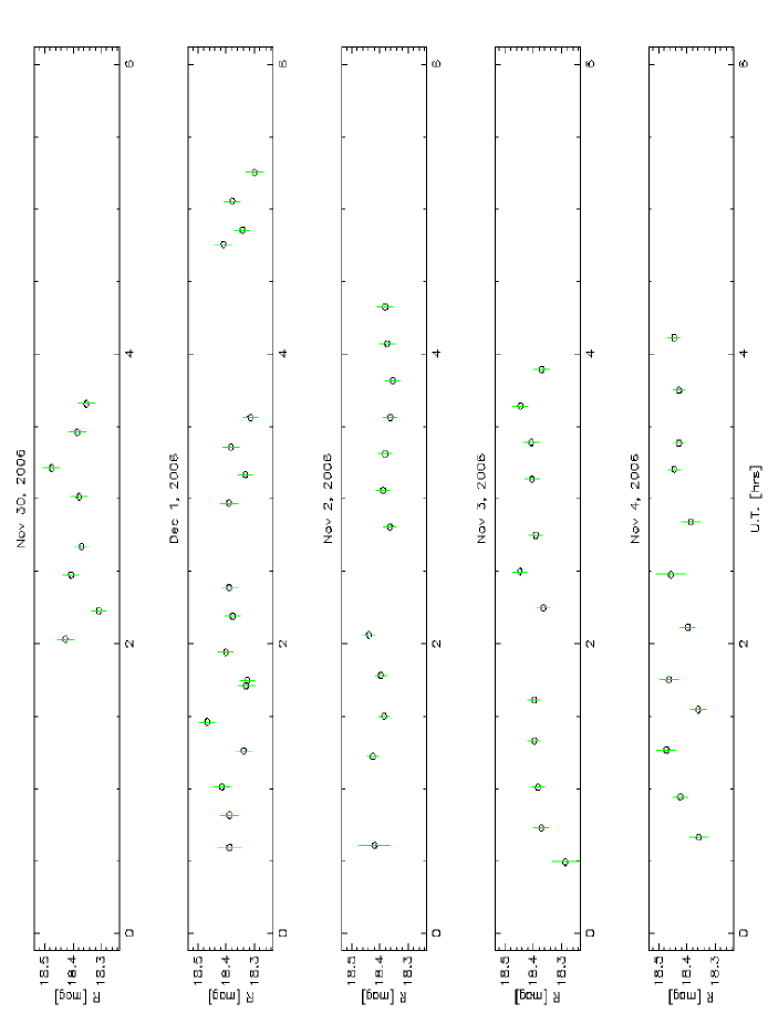
Figure 2: R Light curves of Eris (2003 UB313). From the top to the bottom the light curve for Nov. 30 to Dec. 4, 2005 are shown.

If this tiny time dependence is not due to some unaccounted problem in the data, would be this a sign of an aliasing with short term variability? We attempt to assess whether the dispersion in the data can be ascribed to some periodical variations in the light curve over periods shorter than 5 nights. The phase dispersion minimization method applied to data binned in chunks of 1 hour, favors periodicity of about 30 hrs. Other possible periods are much sensitive to the details of the method, as the number of phase bin or the step in periods. An inspection of data plotted as a function of phase for a 30 hrs periods suggests a scattered, non sinusoidal light curve, with maximum peak-to-peak variation of $\approx 0.06$ mag and a single maximum, but the fitting is marginal ($\chi^{2}=116.74$ with c.l. $=2\times 10^{-5}$ that deviations from the fit are not just due to random errors). The periodogram of data does not allow us to identify any noticeable periodicity between 1 and 100 hours. This is true even after exclusion of periods heavily affected by aliasing (6 hrs, 8 hrs, 12 hrs, 24 hrs and 48 hrs). In particular the 30 hrs period is just outside the 24 hrs side-lobe and the improvement in the $\chi^{2}$ for fitting data with an $\approx 30$ hrs period is again marginal. To have a more robust test we play numerical experiments with simulated sinusoidal signals plus noise. Here we consider periods in the range $1-100$ hrs, amplitudes $\leq 0.05$ mag, constant $R$ magnitude in the $\pm 5\sigma$ of our data and phases in the range $0-2\pi$. Simulated data has been re-binned on a night-by-night basis and compared to night averaged data computing the corresponding $\chi^{2}_{\mathrm{sin}}$. As a comparison we take $\chi^{2}_{\mathrm{sin}}$ with $\chi^{2}_{\mathrm{const}}$, $\chi^{2}_{\mathrm{linear}}=2.36$ (computed over 5 nights) and $\chi^{2}_{\mathrm{parabolic}}$ as defined before. Our results show no significant improvement in the fit by assuming a sinusoidal signal in the data. In at most $3\%$ of our $3\times 10^{5}$ simulated realizations we obtained $\chi^{2}_{\mathrm{sin}}<\chi^{2}_{\mathrm{const}}$. The fraction drops to $0.05\%$ and $0.003\%$ respectively for $\chi^{2}_{\mathrm{sin}}<\chi^{2}_{\mathrm{linear}}$ and $\chi^{2}_{\mathrm{sin}}<\chi^{2}_{\mathrm{parabolic}}$. To have an extreme case of non-sinusoidal signal we consider also the case of a square wave with variable amplitude, period, phase and duty-cycle obtaining a largely worst fit. In conclusion the long term variability in our data can not be explained by aliasing of an under-sampled short term variability.

4 Colors

We computed weighted mean colors of Eris. These are derived from the weighted mean of all the measures in each filter. We obtain $B-V=0.823\pm 0.023$, $V-R=0.391\pm 0.023$, $R-I=0.386\pm 0.012$ and $V-I=0.777\pm 0.013$, quite in agreement with Rabinowitz et al. (2006, Tab. 4). Following the same vein of the discussion in this paper, we confirm that the colors of ERIS are solar, with only B-V being marginally redder than the Sun (Hainaut & Delsanti, 2002). These colors corroborate the idea that Eris is an icy body.

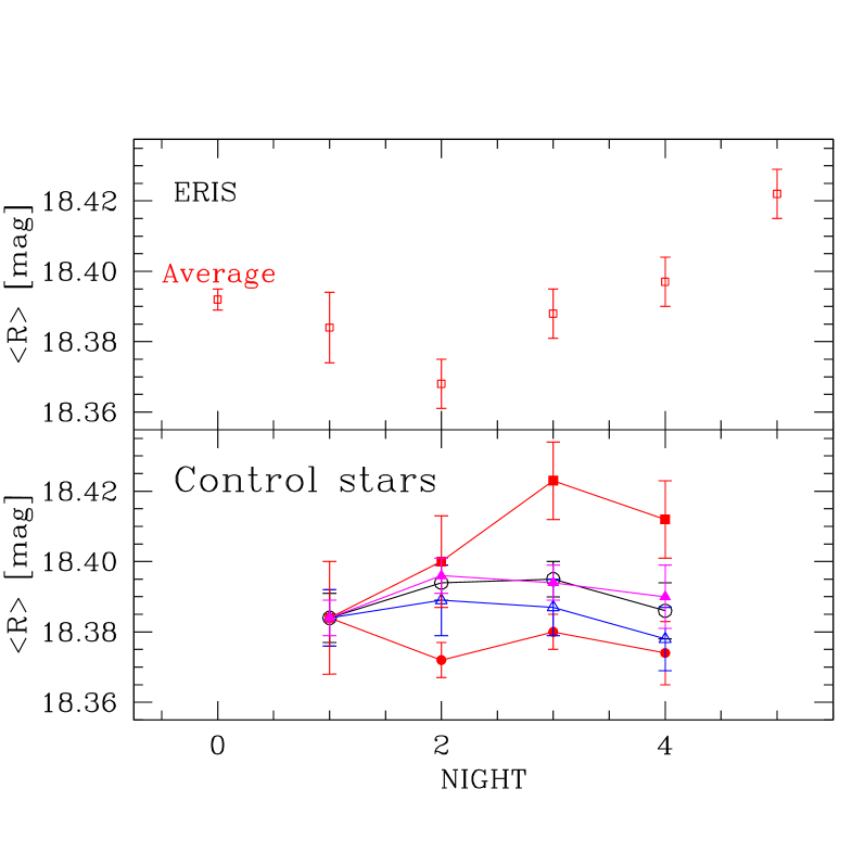
Figure 3: Upper Panel: Eris weighted averages R mag as a function of night (see Tab. 1). The point in blue (dark gray in bw print) at night 0 is the weighted average over the 5 nights.Lower panel: Weighted averages of R as a function of the night for the 5 field stars discussed in the text. Only the data for the first 4 nights are plotted, since the fifth was not photometric. The magnitude of these stars have been arbitrarily shifted to the first night Eris averarge R mag.

5 Discussion and Conclusions

We have presented time series photometry in BVRI pass-bands of the dwarf planet Eris (2003 UB313).
Looking at the data we have presented and analysed (in particular V and R), it is possible to say that some genuine time variability is present with a reasonable level of confidence. If this will be confirmed by further observations it would indicate a light curve with a long term variability. Likely, one with periods greater than 5 days and amplitudes $\approx 0.05$ mag. Such a small amplitude would indicate a low axial ratio for Eris or that this body is seen nearly pole-on from the Earth.
In the first case Eris would be more symmetric in shape than other known KBOs or Pluto itself.
In the second case, due to the large distance to the Sun, Eris is pole on with respect to the Sun too. Presently Eris is near its aphelion and if it has an axial ratio comparable to that of Pluto, we should expect that the maximum amplitude of its light curve would be observed toward the epoch in which it will have an anomaly of $\approx 90^{\circ}$. However, even a change of $10^{\circ}$ in its orientation would produce a significant increment in the amplitude of its light curve.
Interestingly enough for the evolution of resurfacing is the fact that in case Eris were seen pole-on at aphelion, it would have to be pole-on even at perihelion. Having a so large orbital ellipticity, the solar irradiation at aphelion would be 6.6 times smaller than the irradiation at perihelion. Depending on the details of resurfacing mechanism and atmospheric circulation, it would not be a surprise to discover significant differences between the two hemispheres of Eris. As an example, one can speculate that the region of the aphelion pole would be more rich in volatiles than the opposite region. If so, even the spectroscopic signature of the Eris surface will have to show secular variations correlated with the light-curve amplitude.
Finally, in trying to understand Eris light curve, one cannot neglect that the presence of the un-resolved satellite could distort it. Dysnomea indeed may contribute for up to $\approx 0.02$ mag to the time variability of brightness with an expected orbital period of 2 weeks. However, even assuming that the line of nodes of the orbit of the satellite is oriented toward the Sun, an eclipse or a transit would last for about one tenth of day, compatible with the time scale of our observations over each night. But an eclipse or a transit would cause a drop in brightness while our data suggest rather the opposite behavior. In addition, an eclipse or a transit would affect only one night and not the subsequent ones due to the small phase angle with which we are observing the system.

- (1)
- Brown et al. (2005) Brown, M.E., Trujillo, C.A., Rabinowitz, D.L., 2005, ApJ, 635, L97
- Brown et al. (2006a) Brown, M.E., van Dam, M.A., Bouchez, A.H., Campbell, R.D., Chin, J.,Y, Conrad, A., Hartman, S.K., Johansson, E.M., Lafin, R.E., Rabinowitz, D.L., Stomski, Jr., Summers, D.M., Trujillo, C.A., Wizinowich, P.L., 2006a, ApJ, 639, L43
- Brown et al. (2006b) Brown, M.E., Schaller, E.L., Roe, H.G., Rabinowitz, D.L., Trujillo, C.A., 2006, preprint
- Hainaut & Delsanti (2002) Hainault, O.R., Delsanti, A.C., 2002, A&A 389, 641
- IAU (2006) IAU resolution no 5A, 26th IAU General Assembly, Prague 2006
- Licandro et al. (2006) Licandro, J.; Grundy, W. M.; Pinilla-Alonso, N.; Leisy, P., 2006, A&A, 458, L5
- Sheppard (2006) Sheppard, S. S., 2006, Nature, 439, 541
- Rabinowitz et al. (2006) Rabinowitz, D.L., Schaefer, B.E., Tourtellotte S.W., 2006, preprint, astro-ph/0605745