A Method for Extracting Light Echo Fluxes Using the NN2 Difference Imaging Technique

Abstract

Light echoes are interesting because of the wealth of information they offer about their progenitors and the reflecting dust. Due to their faint surface brightnesses, difference imaging is necessary to separate most light echoes from the sky background. However, difference images reveal only the relative fluxes between two epochs. Obtaining absolute fluxes for individual epochs has traditionally relied on a single template image that is free of light echoes. Since such an observation is normally unavailable, a light echo-free template must be constructed by a complicated and usually subjective process. Here we present an application of the NN2 method of Barris et al. to extract the relative fluxes of light echoes across a range of epochs directly from a series of difference images. This method requires no privileged image and makes maximal use of the observational data. Statistical methods to estimate the zero-flux level and thus the absolute flux are also presented. The efficacy of the technique is demonstrated by an application to the light echoes around SN 1987A. The resulting images reveal new detail and faint light echo structures. This method can be adapted and applied to other extended variable light sources, such as stellar outflows and supernova remnants.

1 Introduction

Light echoes arise when light from a stellar event is reflected toward the observer by intervening dust. The arrival of the light is delayed by the extra distance it traverses and so may be observed long after the source event. Light echoes provide a powerful tool for studying interesting stellar phenomena and sensitively probing dust structures. For many dust geometries of interest, the light echoes appear as rings or arclets which usually expand superluminally (Couderc, 1939). Light echoes from variable stars have been observed, including Nova Persei 1901 (Ritchey, 1901), the source of the first discovered light echo, and the mysterious eruptive variable V838 Monocerotis (e.g., Munari et al., 2002; Bond et al., 2003). However, only supernovae (SNe) have sufficient luminosity to produce observable scattering from interstellar dust (Sugerman, 2003). Most light echo discoveries, therefore, have been associated with SNe, including SN 1991T (Schmidt et al., 1994), SN 1993J (Sugerman & Crotts, 2002), SN 1998bu (Cappellaro et al., 2001), SN 2003gd (Sugerman, 2005), and most famously SN 1987A, whose light echoes have been used to investigate in detail the geometry, density, and composition of the circumstellar and interstellar media (Crotts & Kunkel, 1991; Xu et al., 1994, 1995; Crotts et al., 1995; Xu & Crotts, 1999; Sugerman et al., 2005). Contributions from light echoes may significantly affect the observed light curves of Type II SNe (e.g., Chugai, 1992; Di Carlo et al., 2002). Polarization measurements of light echoes can provide an independent distance measurement when scattering is nearly $90^{\circ}$ (Sparks, 1994, 1996). Rest et al. (2005b) have analyzed the spectra of light echoes from ancient SNe to determine the types of their progenitors. Although the wealth of information they contain has inspired searches (e.g., Boffi et al., 1999), most light echoes are difficult to image due to their low surface brightnesses.

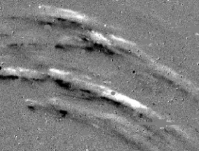
Figure 1: Sample difference image showing 2005 December 31 (image epoch) minus 2005 January 7 (template epoch). White pixels are positive and thus enriched in the image epoch, while black pixels are negative and enriched in the template epoch. Note that this image contains light echo fluxes from both epochs which frequently overlap and exhibit partial cancellation. The FOV is $3.1^{\prime}\times 2.3^{\prime}$.

Sophisticated difference imaging techniques (e.g., Tomaney & Crotts, 1996; Alard & Lupton, 1998; Alard, 2000; Sugerman et al., 2005; Rest et al., 2005b) allow light echoes to be cleanly separated from the sky background, but difference imaging alone can reveal only the relative flux between two epochs. Each difference image shows the flux difference between an image epoch and a template epoch. If a light echo-free image is available, it can serve as a template that can be subtracted from every epoch to isolate the light echoes. Unfortunately, such an observation usually does not exist. Previous studies (e.g., Xu et al., 1995; Sugerman et al., 2005) have therefore focused on constructing a light echo-free image. The construction involves a rather complicated iterative process, requires some subjective decisions, and tends to leak faint light echoes into the echo-free template. Another possibility is to create difference images from epochs that both contain light echo flux. In this case, the sky background is eliminated in the difference image, but both positive and negative light echo fluxes remain. Figure 1 shows a sample difference image in which these positive and negative fluxes are represented by white and black pixels, respectively. Separating these frequently overlapping signals is a serious challenge.

In this paper, we present an application of the NN2 algorithm of Barris et al. (2005) to calculate relative light echo fluxes across a range of epochs directly from a series of difference images. This technique requires no light echo-free template and treats all observations equally. It thus makes maximal use of all the observational data. We also present a statistical method for estimating the zero-flux level of each pixel from the relative light curve, thus determining the absolute flux. The entire procedure is tested on the light echoes around SN 1987A, and the resulting images reveal intricate detail and faint structures.

2 Observations and Reduction

To test the ability of our technique to accurately recover light echo fluxes, the light echoes around SN 1987A were chosen for analysis. Observations were performed by the SuperMACHO survey on the Victor M. Blanco 4m Telescope at Cerro Tololo Inter-American Observatory (CTIO). Imaging of the Large Magellanic Cloud (LMC) was performed every other night in dark time during the months of October, November, December, and January, with occasional images from September and February, during five seasons from 2001 through 2005. These are the months in which the LMC is most visible from Cerro Tololo. We use the $8K\times 8K$ Mosaic II CCD imager with a field of view (FOV) of 0.33 deg², along with a custom broadband VR filter from 500nm to 750nm. For this study, 52 epochs were chosen between 2001 November and 2005 December. These were selected based on transparency, seeing conditions, eccentricity, and their temporal spacing. Images from these $N=52$ epochs were first reduced by the SuperMACHO pipeline. The reduction includes bias correction, cross-talk elimination, flat-fielding, image deprojection, and DoPHOT photometry (Schechter et al., 1993) to compute the zero-point magnitude.

To isolate transient and variable objects such as light echoes, the SuperMACHO pipeline includes difference image analysis. Point spread function (PSF) matched subtraction is performed by the HOTPANTS software (Becker et al., 2004). Since the PSF can vary over the FOV due to optical distortions and imperfect focus, a spatially varying kernel is employed (Alard & Lupton, 1998; Alard, 2000). For more information about the observation program, reduction, and difference imaging, see Rest et al. (2005a).

3 The NN2 Difference Imaging Technique

The principal feature of the NN2 method is that it considers difference images created from all $N(N-1)/2$ possible pairs of observations at $N$ epochs. For this study, the SuperMACHO pipeline was used to produce the 1326 difference images that served as the input to the NN2 algorithm. From the beginning, therefore, we consider images that ideally contain only light echo signal, and the goal is to seperate the positive and negative light echo fluxes contained in these images. The NN2 algorithm is a single-pixel approach. For each pixel, a fit in $N-1$ free parameters is performed to determine the relative fluxes across the $N$ input epochs that best reproduce the flux differences found in the full set of difference images. We thus isolate the light echo signal in each epoch, without the need for an echo-free template. After obtaining the relative fluxes, a separate method is used to establish the absolute flux level for each pixel. Finally, spatial and temporal binning are performed to increase image quality and depth.

3.1 The NN2 Algorithm

The NN2 algorithm was created by Barris et al. (2005) to construct optimal light curves for point-source variable objects from a series of observations. To apply this technique to light echoes, we first consider a single pixel. Let $A$ be the antisymmetric matrix for which $A_{ij}$ is flux in the difference image between epochs $j$ and $i$. This flux is normalized to zero-point magnitude 30, based on the zero-point magnitudes of the images at epochs $j$ and $i$. The matrix $A$, along with an error matrix $E$ whose entries contain the uncertainties in the corresponding entries of $A$, represents the input to the NN2 algorithm from the difference imaging pipeline. We fit $A$ to the form $A_{ij}=V_{j}-V_{i}$ by minimizing

$$\chi^{2}=\sum_{i<j}\frac{(-A_{ij}+V_{j}-V_{i})^{2}}{E_{ij}^{2}}+\frac{\sum V_{i}}{\langle{E}\rangle^{2}},$$ (1)

where $\langle{E}\rangle$ represents the average error, given by

$$\frac{1}{\langle{E}\rangle^{2}}=\frac{2}{N(N-1)}\sum_{i<j}\frac{1}{E_{ij}^{2}}.$$ (2)

The vector $V$ then contains the relative fluxes across the $N$ epochs. The second term in Equation (1) is necessary to obtain a unique solution for $V$, which is otherwise insensitive to the addition of a constant vector. This term implies $\sum V_{i}=0$ and requires us to determine the zero-flux level separately for each pixel. As derived in Barris et al. (2005), $\chi^{2}$ is minimized by solving a system of $N$ linear equations using matrix inversion.

There are two sources of uncertainty in $V$. The “internal error” is due to the fact that $A$ cannot in general be perfectly represented as $A_{ij}=V_{j}-V_{i}$ for any $V$. An estimate for this error arises naturally in the calculation of $V$, as described in Barris et al. (2005). In addition, there are uncertainties in $V$ due to errors $E$ in the difference images, which we call the “external error.” To estimate the external error in $V$, we assume that the uncertainty $E_{ij}$ in the difference image arises from uncertainties $\sigma_{i}$ and $\sigma_{j}$ in the original images at epochs $i$ and $j$, i.e., that there exists a vector $\sigma$ such that

$$E_{ij}^{2}=\sigma_{i}^{2}+\sigma_{j}^{2}.$$ (3)

To calculate the best-fit $\sigma$, we minimize

$$\chi_{e}^{2}=\sum_{i,j;i<j}\left(-1+\frac{\sigma_{i}^{2}}{E_{ij}^{2}}+\frac{\sigma_{j}^{2}}{E_{ij}^{2}}\right)^{2}.$$ (4)

The minimization condition

$$\frac{\partial\chi_{e}^{2}}{\partial\sigma_{k}^{2}}=0$$ (5)

results in a system of $N$ equations, which can be written as

$$\sum_{i;i\neq k}\frac{1}{E_{ik}^{2}}=\sum_{i}D_{ik}\sigma_{i}^{2},$$ (6)

where

$$\displaystyle D_{ik} = \frac{1}{E_{ik}^{4}},\quad i\neq k$$

$$D_{kk} = \sum_{i;i\neq k}\frac{1}{E_{ik}^{4}},$$ (7)

and solved by inverting $D$.

In rare cases, this method yields negative solutions for $\sigma_{i}^{2}$, indicating that the original assumption that $E_{ij}^{2}$ can be well-represented by $\sigma_{i}^{2}+\sigma_{j}^{2}$ is not accurate. In practice, this occurs in of order 1 in $10^{5}$ pixels, which are therefore simply masked. The $\chi_{e}^{2}$ in equation (4) is that adopted in the NN2 code of M. W. Wood-Vasey, J. Tonry, and M. C. Novicki. It differs slightly from the $\chi_{e}^{2}$ given in Barris et al. (2005). In practice, the errors obtained are similar when both methods are available, but minimizing the $\chi_{e}^{2}$ of Barris et al. (2005) fails far more often (i.e., yields negative values for $\sigma_{i}^{2}$).

To compute the total uncertainty, the contributions of both the internal and external errors must be considered. To combine these errors, we use the weighted method presented in Barris et al. (2005), in which the internal error is weighted by the normalized $\chi^{2}$ of equation (1).

For the heart of the NN2 calculation, the antivec function, we adapted the code of W. M. Wood-Vasey, J. Tonry, and M. C. Novicki. A region of specified size is read into memory from each of the $N(N-1)/2$ difference images. For each pixel, masked data are discarded as follows. The number of images associated with each epoch (either as the image or template date) in which the pixel is masked is calculated. All images associated with the epoch having the highest count are discarded, and the process is repeated until no masked data remains. We consider input pixels as masked if they are marked by the SuperMACHO pipeline as saturated or bad pixels. The NN2 algorithm is run with the remaining data, and a crude zero-flux level is set by shifting the relative fluxes so that the minimum flux for each pixel is zero. Image files containing the flux, internal error, external error, and total error are created. In addition, mask files are created for each epoch showing which pixels were discarded. Pixels that encountered an error in calculating the external error are also flagged. From the mask files, an image is created, indicating the total number of epochs included in the calculation for each pixel. Pixels calculated with fewer than 30 epochs were masked in our study of SN 1987A.

3.2 Zero-Flux–Level Determination

Since the NN2 algorithm provides only relative fluxes, the light curves obtained for each pixel contain arbitrary offsets with respect to both the true zero-flux level and the neighboring pixels. It is therefore necessary to estimate the true zero-flux level for each pixel. Figure 2a shows the relative light curve of an example pixel as determined by the NN2 algorithm. As a first crude estimate, the zero-flux level is taken to be the minimum flux over all epochs. This value is subtracted from each epoch to produce Figure 2a. Since our observations were taken in annual spans of approximately 3 months for 5 years, we group the data into five seasons. The example in Figure 2 shows a very faint light echo in the third season. In order to estimate the zero-flux level, we must identify the time periods (in our case, seasons) that contain no light echo flux. For faint light echoes, as in this example, this is very difficult, because the individual pixel values are sometimes barely 1 $\sigma$ above the sky background. To assist in identifying the zero-flux epochs, we use the following properties of light echoes:

• Light echoes are spatially extended, so nearby pixels are very likely to share the same epochs with zero light echo flux. Thus, we can spatially bin the fluxes by replacing each pixel with the weighted mean of its unmasked neighbors within a $3\times 3$ box, excluding the highest and lowest fluxes. (Throughout this paper, extreme fluxes are excluded from means only when at least six data points are available.) The resulting spatially-smoothed light curve is shown in Figure 2b.

• In most cases, light echoes do not change significantly over a time scale of months. Thus we can temporally bin the fluxes as well. In our case, the five seasons form the natural binning periods. Within each season, the epochs of highest and lowest flux are excluded. These are denoted by crosses in Figure 2b. Using the remaining data, the weighted mean flux of each season is calculated. These are shown as squares in Figure 2. In this example, the mean of the spatially-binned third season is $6.4$ $\sigma$ above the mean of the other four seasons. Without spatial binning, this is reduced to $2.6$ $\sigma$.

Using the spatially- and temporally-binned light curve, we use the following algorithm to determine the seasons that contain zero light echo flux:

• Seasons whose mean is more than 3 $\sigma$ above the minimum mean among all seasons are considered to contain light echoes and are thus excluded. In practice, most seasons that will be cut are excluded by this sigma cut.

• Seasons that exhibit a strong gradient are excluded. The presence of a gradient is detected by measuring how well the best-fit line fits the data compared to a flat line at the mean. In particular, the ratio of the $\chi^{2}$ statistic for the mean to the $\chi^{2}$ statistic for the best-fit line, as determined by the least-squares method, is calculated. Seasons for which this ratio exceeds 10 are cut.

• Seasons with a normalized $\chi^{2}$ greater than 3.5 are excluded.

The remaining seasons are deemed to contain zero light echo flux. In the example of Figure 2, these are seasons 1, 2, 4, and 5. (Season 3 is excluded by the sigma cut.) Since at least one season must be used to calculate the zero-flux level, none of the above steps is allowed to exclude all the remaining seasons. If one initially does so, the parameter being measured is examined, and the season that deviates least from a perfect zero-flux season is retained. The critical values of the parameters in the second and third steps were chosen by sampling pixels from regions containing passing light echoes and choosing values to best reproduce the zero-flux level seen in the light curve. They can be adjusted for different data sets; however, since the second and third steps are included as safeguards after the dominant sigma cut, the exact critical values are not likely to significantly affect the output.

Having determined the zero-flux seasons, we use this information to correct the original, unbinned light curve, shown in Figure 2a. For each zero-flux season, the highest and lowest fluxes are cut to reduce the influence of outlier data. (We deemed this cut sufficient for our data. Those planning future applications may want to consider an iterative sigma clip instead.) The weighted mean of all zero-flux seasons is taken to be the zero-flux level, shown by the dotted line in Figure  2a. This value is subtracted from the flux at every epoch, and its uncertainty is combined quadratically with errors in the fluxes, to produce the zero-flux corrected light curve, as shown in Figure 2c.

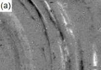
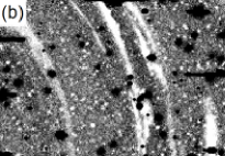
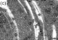
Figure 3: (a) Difference image with image and template epochs of 2004 December 13 and 2001 December 11, respectively. (b) NN2 output for the image epoch of the difference image. For each pixel, the relative light curve obtained from the NN2 algorithm is shifted so that the minimum flux over all epochs is zero. Note that light echo flux from the template epoch in (a) has been eliminated. (c) Zero-flux–corrected image for the same epoch. Each pixel level has been shifted to the proper flux zero point. The FOV is $3.0^{\prime}\times 2.0^{\prime}$.

The results of this method, applied not only to a single pixel but to an entire region, are shown in Figure 3. Panel a shows a difference image, panel b shows the NN2 output for the image epoch of the difference image, and panel c shows the zero-flux–corrected image for the same epoch. Note how much more clearly the light echoes appear above the sky background in panel c, especially the fainter features.

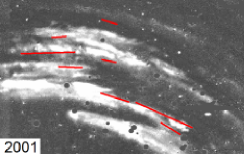
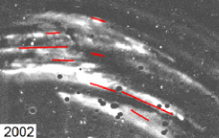
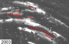
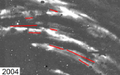
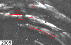
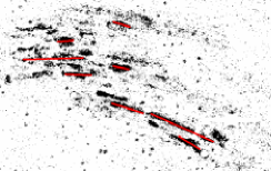
Figure 4: Mean-combined images for the 2001–2005 seasons showing a region with closely spaced light echo arcs. The final frame shows those pixels for which only one zero-flux season is identified. The close spacing of the light echo arcs in this region causes an unusually high number of pixels to contain light echoes in all but one season. For these pixels, the flux values obtained here may be only lower limits on the true flux. The red lines are constant in each image and highlight areas dense in pixels with one zero-flux season. Note that every such pixel necessarily has a calculated flux of zero in one season, even if light echoes were physically present throughout the observation period. By following the motion of the light echoes, however, we can generally exclude this possibility. The FOV is $3.5^{\prime}\times 2.2^{\prime}$.

The procedure described here is dependent on the availability of true zero-flux epochs in the neighborhood of every pixel. For some pixels, only one season is identified as containing zero light echo flux. For them, it is possible that all seasons actually contain light echoes, and that the identified season really contains the faintest light echo region, rather than zero flux. In this case, the calculated zero-flux level is an overestimate of the true value, and the fluxes obtained are lower limits on the true fluxes. In our example of SN 1987A, the rings move quickly enough and are thin enough that few pixels should contain light echoes for 5 consecutive years. However, there are some regions that contain several closely spaced light echo arclets. An extreme case is shown in Figure 4, in which the final frame indicates those pixels with only one zero-flux season identified. The red lines are constant and indicate regions that are dense in such pixels. It is possible that some of these pixels are illuminated by light echoes throughout the observation period. The season during which the faintest echoes pass is used to calculate the zero-flux level, and consequently the light echoes disappear from the zero-flux–corrected images for that season. This effect must be accounted for, especially if the technique presented here is applied to light echoes with more complicated structure.

In our images of SN 1987A, 7% of all usable pixels have only one zero-flux season identified. In all cases we have examined, this season does seem to represent the true zero-flux level. Sometimes this can be verified from the light curve. Figure 5 shows the zero-flux–corrected light curve for a pixel containing a very bright light echo. Despite being the only zero-flux season identified, the first season does appear to contain zero light echo flux. Pixels with only one zero-flux season can also be inspected by following the motion of light echo arcs. If the zero-flux season falls in a gap between arcs that appears in images from the other seasons, we can be confident in its veracity. If, on the other hand, a conspicuous hole were to appear in the zero-flux season, altering the shape of the light echo, the calculated fluxes would be interpreted as lower limits.

3.3 Stacking and Smoothing

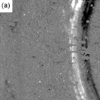
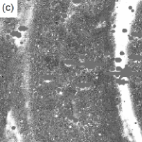
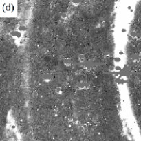
Figure 6: Stages of light echo extraction showing a region containing a weak light echo arc in the left part of the frame. The FOV is $2.9^{\prime}\times 2.9^{\prime}$. (a) Difference image showing 2004 December 15 minus 2001 December 21. (b) Zero-flux corrected image for 2001 December 21. This is the template epoch of the difference image, in which it appears black. (c) Mean-combined image for the 2001 season. (d) Smoothed mean-combined image for the same season.

To assist in separating very faint light echo pixels from the sky background, the NN2 images from each season were mean-combined (stacked), excluding masked epochs as well as those containing the highest and lowest fluxes, resulting in five stacked images. Corresponding error and mask images were also created. Since the flux can change by a factor of 2 or more within a single season in a region with a moving light echo, this binning reduces the detail contained in the flux information. However, it does increase the signal-to-noise ratio and improve the visibility of faint rings for detection. The number of bad pixels with extreme values is also reduced. These can arise, for example, from difference imaging artifacts in the original difference images. To further improve visibility, the five stacked images were smoothed using the same spatial binning technique described in section 3.2. The results are shown in Figure 6. Panels a and b show a sample difference image and the zero-flux–corrected output for its template epoch, respectively. Panel c shows the season mean-combined image, formed by stacking many images like the one in b, and d shows the same image after spatial smoothing. The stacking and smoothing procedure typically increased the signal-to-noise ratio by a factor of 10 in our images of SN 1987A. This could be anticipated, since stacking should reduce the noise by a factor of approximately $(N/n)^{1/2}$, where $n$ is the number of seasons, and smoothing should further reduce the noise by a factor of $\sqrt{s}$, where $s$ is the number of pixels used in the smoothing kernel. In this case, $N=52$, $n=5$, and $s=9$, so $(Ns/n)^{1/2}\approx 10$.

4 Discussion

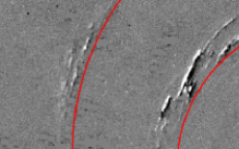
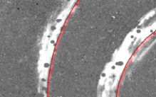
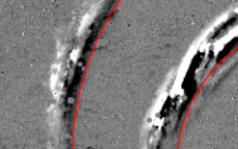
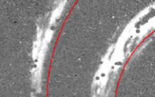
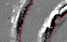
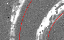
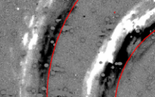
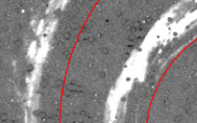
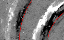
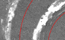
Figure 7: Left column: Difference images with template epoch 2001 November 15 and image epochs 2001 December 11, 2002 December 14, 2003 December 15, 2004 December 15, and 2005 December 21, respectively, from top to bottom. Right column: Zero-flux–corrected images for the same five image epochs. The red arcs provide a constant point of reference. In each difference image, the light echo positions in the image and template epochs overlap, causing partial or complete cancellation. The NN2 algorithm disentangles this information to reveal the complete extent of the light echoes. Note especially in the first image the near complete cancellation evident in the difference image, in which the image and template dates are separated by only 1 month. Compare this to the image on the right. The FOV is $3.0^{\prime}\times 2.0^{\prime}$.

Figure 7 shows the evolution of one light echo region over our five seasons of observation. The left column shows difference images with the same template epoch in 2001 November. The image epochs are separated by 1 year and fall in December 2001, 2002, 2003, 2004 and 2005. The right column shows the zero-flux–corrected NN2 images for the same five epochs. Note that in the first difference image, the template and image dates are separated by less than 1 month. The light echoes move very little during this short interval, so the difference image shows almost complete cancellation between the light echoes at the two epochs. However, the accompanying zero-flux–corrected NN2 image shows the full extent of the light echo. The second and subsequent difference images show some regions that appear to contain flux only from the image epoch, and others that appear to contain flux only from the template epoch. However, it is difficult to make these judgments with certainty, and there are always significant regions of overlap, in which the difference image reveals only the change in flux. The NN2 algorithm allows us to disentangle this information and extract the relative light echo fluxes across a range of epochs rather than only two. It is important to note that the images in the right column of Figure 7 are not obtained directly from the accompanying difference images, but rather depend on all $N(N-1)/2$ difference images obtained from the $N$ observations. This figure clearly shows the limitations of the single-template difference imaging method and the advantages offered by the NN2 algorithm.

In addition to uncovering the spatial extent of light echoes, our technique can reveal faint light echo features not visible in the difference images. Figure 6 shows stages of analysis for a region containing a faint light echo ring in the left part of the frame. Note that this ring is barely tracable in the sample difference image. In our full mean-combined images, light echo features with peak surface brightnesses of 25 mag arcsec^-2 are clearly visible, whereas the light echo detection limit in the difference images is about 24 mag arcsec^-2.

Our code, along with images from an example region around SN 1987A, are available online. The NN2 calculations involve several large matrix inversions and are CPU-intensive. Our Python code required roughly 30 hours on 20 CPUs to process 52 images of dimensions $4160\times 1100$. Although vast speed improvements can likely be expected from C code, the processing demands should be borne in mind when considering larger scale applications.

5 Conclusions

Difference imaging is a standard tool in the analysis of light echoes. Without a light echo-free template, however, difference images contain overlapping light echo fluxes from two epochs. We present here a new method that produces images containing absolute light echo fluxes from one epoch only. The NN2 algorithm is used to calculate a relative light curve across a range of $N$ epochs by considering difference images constructed from every pair of epochs. By applying this method over a region, we obtain light curves for each pixel. However, these lightcurves have arbitrary offsets with respect to each other and to the true zero-flux level. Hence, we apply a statistical method to estimate the true zero-flux level for each pixel and shift the light curves accordingly. This method is optimized for detecting faint light echoes with peak surface brightnesses as faint as 25 mag arcsec^-2. By spatially and temporally binning the images, we greatly increase the signal-to-noise ratio. Our technique is capable of revealing fine structure and faint light echo regions. It requires no privileged or light echo-free images and can be applied completely automatically to a wide variety of light echo situations. In addition, variations on this technique could permit analysis of other extended variable light sources, such as stellar outflows and supernova remnants. Future work will include applications to recently discovered light echoes from ancient supernovae in the Large Magellanic Cloud (Rest et al., 2005b).

6 Acknowledgments

The SuperMACHO survey is being undertaken under the auspices of the NOAO Survey Program. We are very grateful for the support provided to the Survey program from the NOAO and the National Science Foundation. A. Rest thanks NOAO for the Goldberg Fellowship. SuperMACHO is supported by the STScI grant GO-10583 and GO-10903. Discussions with Michael Wood-Vasey were very valuable. A. Newman thanks the National Science Foundation for their support via the Research Experience for Undergraduates (REU) program. We thank the referee B. Sugerman for very useful comments and suggestions which helped improve the quality of this paper.

Figure 2: Light curves for a pixel containing a faint light echo in season 3. (a) Relative fluxes obtained from the NN2 algorithm. (b) Smoothed fluxes obtained by spatially binning pixels in a $3\times 3$ box. The crosses denote the highest and lowest flux values from each season, which are excluded in calculating the season means, denoted by squares. A light echo is identified in season 3 by the sigma cut, and the remaining four seasons are deemed to represent the zero-flux level. The dotted line shows their mean. (c) Zero-flux–corrected light curve. The mean of the unbinned fluxes in the zero-flux seasons is set as the zero-flux level, the dotted line in (a). This is subtracted from each epoch to produce the corrected light curve here. Squares and crosses have the same meaning as above. Error bars show the 1 $\sigma$ uncertainties.

Figure 5: Zero-flux–corrected light curve for a pixel containing a bright light echo. Seasons 2 through 5 are excluded by the sigma cut, and the zero-flux level is determined by season 1 alone. Nevertheless, given the smooth nature of the curve and the flatness of the season 1 data, it is very likely that season 1 represents the true zero-flux level. Uncertainties are comparable to the size of the points.

References

- Alard (2000) Alard, C. 2000, A&AS, 144, 363
- Alard & Lupton (1998) Alard, C., & Lupton, R. H. 1998, ApJ, 503, 325
- Barris et al. (2005) Barris, B. J., Tonry, J. L., Novicki, M. C., & Wood-Vasey, W. M. 2005, AJ, 130, 2272
- Becker et al. (2004) Becker, A. C., et al. 2004, ApJ, 611, 418
- Boffi et al. (1999) Boffi, F. R., Sparks, W. B., & Macchetto, F. D. 1999, A&AS, 138, 253
- Bond et al. (2003) Bond, H. E., et al. 2003, Nature, 422, 405
- Cappellaro et al. (2001) Cappellaro, E., et al. 2001, ApJ, 549, L215
- Chugai (1992) Chugai, N. N. 1992, Soviet Astronomy, 36, 63
- Couderc (1939) Couderc, P. 1939, Annales d’Astrophysique, 2, 271
- Crotts & Kunkel (1991) Crotts, A. P. S., & Kunkel, W. E. 1991, ApJ, 366, L73
- Crotts et al. (1995) Crotts, A. P. S., Kunkel, W. E., & Heathcote, S. R. 1995, ApJ, 438, 724
- Di Carlo et al. (2002) Di Carlo, E., et al. 2002, ApJ, 573, 144
- Munari et al. (2002) Munari, U., et al. 2002, A&A, 389, L51
- Rest et al. (2005a) Rest, A., et al. 2005a, ApJ, 634, 1103
- Rest et al. (2005b) Rest, A., et al. 2005b, Nature, 438, 1132
- Ritchey (1901) Ritchey, G. W. 1901, ApJ, 14, 293
- Schechter et al. (1993) Schechter, P. L., Mateo, M., & Saha, A. 1993, PASP, 105, 1342
- Schmidt et al. (1994) Schmidt, B. P., Kirshner, R. P., Leibundgut, B., Wells, L. A., Porter, A. C., Ruiz-Lapuente, P., Challis, P., & Filippenko, A. V. 1994, ApJ, 434, L19
- Sparks (1994) Sparks, W. B. 1994, ApJ, 433, 19
- Sparks (1996) Sparks, W. B. 1996, ApJ, 470, 195
- Sugerman (2003) Sugerman, B. E. K. 2003, AJ, 126, 1939
- Sugerman (2005) Sugerman, B. E. K. 2005, ApJ, 632, L17
- Sugerman & Crotts (2002) Sugerman, B. E. K., & Crotts, A. P. S. 2002, ApJ, 581, L97
- Sugerman et al. (2005) Sugerman, B. E. K., Crotts, A. P. S., Kunkel, W. E., Heathcote, S. R., & Lawrence, S. S. 2005, ApJS, 159, 60
- Tomaney & Crotts (1996) Tomaney, A. B., & Crotts, A. P. S. 1996, AJ, 112, 2872
- Xu & Crotts (1999) Xu, J., & Crotts, A. P. S. 1999, ApJ, 511, 262
- Xu et al. (1994) Xu, J., Crotts, A. P. S., & Kunkel, W. E. 1994, ApJ, 435, 274
- Xu et al. (1995) Xu, J., Crotts, A. P. S., & Kunkel, W. E. 1995, ApJ, 451, 806