The Clustering of Galaxy Groups: Dependence on Mass and Other Properties

Abstract

We investigate the clustering of galaxy groups and clusters in the SDSS using the Berlind et al. (2006) group sample, which is designed to identify galaxy systems that each occupy a single dark matter halo. We estimate group masses from their abundances, and measure their relative large-scale bias as a function of mass. Our measurements are in agreement with the theoretical halo bias function, given a standard $\Lambda$CDM cosmological model, and they tend to favor a low value of the power spectrum amplitude $\sigma_{8}$. We search for a residual dependence of clustering on other group properties at fixed mass, and find the strongest signal for central galaxy color in high mass groups. Massive groups with less red central galaxies are more biased on large scales than similar mass groups with redder central galaxies. We show that this effect is unlikely to be caused by errors in our mass estimates, and is most likely observational evidence of recent theoretical findings that halo bias depends on a “second parameter” other than mass, such as age or concentration. To compare with the data, we study the bias of massive halos in N-body simulations and quantify the strength of the relation between halo bias and concentration at fixed mass. In addition to confirming a non-trivial prediction of the $\Lambda$CDM cosmological model, these results have important implications for the role that environment plays in shaping galaxy properties.

1. Introduction

Our current understanding of galaxy formation is centered on the well-motivated assumption that all galaxies are formed and live their lives within dark matter halos. The observed clustering of galaxies is thus tied to the clustering of halos. Indeed, the modern way of modeling galaxy clustering is to combine halo profiles, abundances, and clustering (measured from cosmological N-body simulations) with prescriptions (usually referred to as the halo occupation distribution) that specify how galaxies occupy halos (e.g., Seljak 2000; Peacock & Smith 2000; Scoccimarro et al. 2001; Berlind & Weinberg 2002; Cooray & Sheth 2002). These halo models usually assume that the large-scale clustering of halos depends only on halo mass. Under this assumption, galaxy properties only correlate with large-scale environment via their correlation with halo mass.

The dependence of halo clustering on mass has been studied extensively in the context of $\Lambda$CDM cosmological models and is fairly well understood (e.g., Cole & Kaiser 1989; Mo & White 1996; Sheth & Tormen 1999; Seljak & Warren 2004; Tinker et al. 2005). Moreover, the exact form of this dependence is sensitive to the values of cosmological parameters, such as the mass density $\Omega_{m}$ and the amplitude of the matter power spectrum $\sigma_{8}$, and can thus, in principle, be used to constrain cosmological models.

Recent studies using N-body simulations have shown, however, that the clustering of halos also depends on a second parameter, in addition to halo mass. Sheth & Tormen (2004) first noted this when they detected that halos in dense environments formed at slightly earlier times than halos of the same mass that are in low density environments. Gao et al. (2005) and then Harker et al. (2006) explored this in a larger simulation and found a much stronger signal: early forming halos cluster more strongly on large scales than late-forming halos of the same mass. This effect, sometimes referred to as “assembly bias”, was strongest for halos of mass much less than the nonlinear mass $M_{\ast}$, and it disappeared for larger masses. Wechsler et al. (2006) did a more thorough analysis of these issues and, in addition to confirming the Gao et al. (2005) result at low masses, found the opposite effect for high mass halos, with a turnaround at $M\sim M_{\ast}$. High mass halos that have recently assembled cluster more strongly than old halos of the same mass. Wechsler et al. (2006) also showed that all these effects persist when using halo concentration, rather than age, as the “second parameter”. This is not surprising given that halo concentration correlates with formation time (Wechsler et al. 2002). Finally, Wetzel et al. (2006) studied the high mass regime in detail and confirmed the Wechsler et al. (2006) results.

The correlation of large-scale environment with halo age/concentration at fixed mass will propagate into a correlation with galaxy properties if these properties themselves correlate with halo age/concentration at fixed mass. Croton et al. (2006) studied this issue in a semi-analytic model and found that the clustering of red and blue model galaxies on large scales cannot be explained solely by the color-mass and mass-clustering relations. In other words, galaxy color must also correlate with large-scale environment through a “second parameter” like halo age or concentration. This may not be surprising, but observational analyses have shown that, in the real universe, if these effects exist they are quite small (Abbas & Sheth 2006; Skibba et al. 2006; Blanton & Berlind 2006). The apparent discrepancy between the theoretical and observational studies could be due to the fact that the predicted effects for halos are only strong for either (1) very low mass halos that do not contain galaxies luminous enough to be included in the observational samples, or (2) very high mass halos that are rare and do not contribute much to the total observed clustering of galaxies. Alternatively, it is possible that the trends seen for halos do not, in fact, propagate into trends for galaxies and that the Croton et al. (2006) results do not apply to the real universe. It is worth noting that the semi-analytic model used in this study does not predict the correct clustering of red and blue galaxies (Springel et al. 2005).

A more direct way of observationally probing the theoretical results is to study not galaxies, but groups and clusters of galaxies, because these are the objects that presumably correspond one-to-one with halos. Given a galaxy luminosity limit near $L_{\ast}$, which is typical for current large surveys, low mass halos ($M\sim 10^{12}M_{\odot}$) will contain one isolated galaxy, intermediate mass halos ($M\sim 10^{13}M_{\odot}$) will contain a group of galaxies, and high mass halos ($M\sim 10^{14}M_{\odot}$) will contain a cluster. Studying the clustering of groups can thus serve as a proxy for studying halos. In particular, we want to look for an observed group property that acts as a “second parameter” and shows a clustering dependence at fixed mass. Many studies have focused on measuring the clustering of groups as a function of properties that act as a proxy for mass (Bahcall & Soneira 1983; Giuricin et al. 2000; Bahcall et al. 2003; Padilla et al. 2004; Yang et al. 2005; Coil et al. 2006), but few have looked at other parameters. One notable exception is Yang et al. (2006), who found evidence of such an effect using a group catalog derived from the Two Degree Field Galaxy Redshift Survey (2dFGRS; Colless et al. 2001). Specifically, they found that, at fixed estimated group mass, groups containing central galaxies with low star formation rates (SFR) are more clustered on large scales than groups containing central galaxies with high SFR. Yang et al. (2006) found this result for all group masses in their sample.

In this paper we investigate the clustering of groups in the Sloan Digital Sky Survey (SDSS, York et al. 2000). We use the Berlind et al. (2006) group catalog that was constructed using an algorithm tuned to identify galaxy systems that each occupy a single DM halo. We describe the galaxy and groups samples that we use, as well as our analysis methods in § 2. We first study group clustering as a function of estimated mass in § 3, and then search for a residual dependence on other group properties in § 4. In § 5 we analyze the clustering of halos in N-body simulations to compare with our group measurements. We discuss and summarize our results in § 6 and 7.

2. Data and Analysis

2.1. SDSS

The SDSS is a large imaging and spectroscopic survey that is mapping two-fifths of the Northern Galactic sky and a smaller area of the Southern Galactic sky, using a dedicated 2.5 meter telescope (Gunn et al. 2006) at Apache Point, New Mexico. The survey uses a photometric camera (Gunn et al. 1998) to scan the sky simultaneously in five photometric bandpasses (Fukugita et al. 1996; Smith et al. 2002) down to a limiting $r$-band magnitude of $\sim 22.5$. The imaging data are processed by automatic software that does astrometry (Pier et al. 2003), source identification, deblending and photometry (Lupton et al. 2001; Lupton 2005), photometric calibration (Hogg et al. 2001; Smith et al. 2002; Tucker et al. 2006), and data quality assessment (Ivezić et al. 2004). Algorithms are applied to select spectroscopic targets for the main galaxy sample (Strauss et al. 2002), the luminous red galaxy sample (Eisenstein et al. 2001), and the quasar sample (Richards et al. 2002). The main galaxy sample is approximately complete down to an apparent $r$-band Petrosian magnitude limit of $<17.77$. Targets are assigned to spectroscopic plates using an adaptive tiling algorithm (Blanton et al. 2003d). Finally, spectroscopic data reduction pipelines produce galaxy spectra and redshifts.

Our group sample is identified from the large-scale structure sample sample14 from the NYU Value Added Galaxy Catalog (NYU-VAGC; Blanton et al. 2005). Galaxy magnitudes are corrected for Galactic extinction (Schlegel et al. 1998) and absolute magnitudes are k-corrected (Blanton et al. 2003a) and corrected for passive evolution (Blanton et al. 2003c) to rest-frame magnitudes at redshift $z=0.1$. The galaxy sample that we use was made publicly available (and superseded) with the SDSS Data Release 4 (Adelman-McCarthy et al. 2006). We restrict our sample to regions of the sky where the completeness (ratio of obtained redshifts to spectroscopic targets) is greater than $90\%$. Our final sample covers 3495.1 square degrees on the sky and contains 298729 galaxies.

2.2. Group and Cluster Samples

We use the group sample described in Berlind et al. (2006). Groups were identified using a redshift-space friends-of-friends algorithm (Geller & Huchra 1983), which was applied to a volume-limited sample of galaxies spanning the redshift range from $z=0.015$ to 0.1 and complete down to an absolute $r$-band magnitude of -19.9 (the $Mr20$ sample in Berlind et al. 2006). This sample contains 57138 galaxies. With the help of mock galaxy catalogs, the group-finding algorithm was tuned to identify galaxy systems that each occupy the same underlying dark matter halo. The result was a group sample that has unbiased richness and size distributions with respect to the underlying halo population. We emphasize that the group-finding algorithm used only the galaxy positions in redshift space and did not use other properties, such as color. The volume-limited sample, mock catalogs, group-finding algorithm, and the resulting group catalog are described in detail in Berlind et al. (2006).

We compute a total $r$-band luminosity for each group by summing the luminosities of its member galaxies. These group luminosities are not actually “total”, since they do not include the light of member galaxies below the -19.9 absolute magnitude threshold. However, since the groups were identified from a volume-limited sample of galaxies, these luminosities should roughly preserve the rank order of true group luminosities. We then obtain masses for our groups by matching the group luminosity function to a theoretical halo mass function, assuming a monotonic relation between group luminosity and mass. Specifically, we use a Warren et al. (2006) halo mass function with the following values for cosmological parameters: $\Omega_{m}=0.3$, $\Omega_{b}=0.04$, $n_{s}=1.0$, $\sigma_{8}=0.9$. We use this slightly outdated cosmological model because the mock catalogs that were used to test the group-finder were based on this model. We thus obtain group mass estimates from their abundances, which Berlind et al. (2006) showed to be unbiased with respect to the abundances of halos. Our mass estimates ignore the scatter in the mass-luminosity relation, but this should not affect our results much because we only use the group masses to create a set of mass-threshold group samples. However, we note that these are actually group luminosity threshold samples, which are characterized as having the same abundance as halos of the stated mass thresholds.

We create four group sub-samples with the following mass thresholds: $\mathrm{log}(M/h^{-1}M_{\odot})>14.0$, 13.5, 13.0, and 12.5. The resulting number of groups in each of these samples is 327, 1316, 4299, and 12655, respectively. Approximately 45% of groups in the mass range $12.5<\mathrm{log}(M/h^{-1}M_{\odot})<13.0$ are isolated galaxies (i.e., $N=1$ groups). On the high mass end, $\sim 90\%$ of groups more massive than $\mathrm{log}(M/h^{-1}M_{\odot})>14.0$ contain 9 or more galaxies.

We define the position of each group on the sky to be the centroid of its member galaxy positions, and the group redshift to be the mean member galaxy redshift. Our results are not sensitive to these choices, since we focus on the clustering of groups on large scales.

2.3. Analysis Method

We wish to measure the relative bias of groups as a function of mass and other group properties. The bias between two samples $A$ and $B$ is typically defined as the large-scale asymptotic value of $\sqrt{\xi_{AA}(r)/\xi_{BB}(r)}$, where $\xi_{AA}(r)$ and $\xi_{BB}(r)$ are the two-point autocorrelation functions of the two samples. However, our group samples are small enough (especially at high masses) that the autocorrelations are very noisy, since the number of group-group pairs is small. We therefore measure cross-correlations of our group samples with the full volume-limited galaxy sample from which the groups were identified. These cross-correlation functions are much higher signal-to-noise because the number of galaxies is much higher than the number of groups. The bias between group samples $A$ and $B$ is now the large-scale asymptotic value of $b(r)=\xi_{AG}(r)/\xi_{BG}(r)$, where $\xi_{AG}(r)$ and $\xi_{BG}(r)$ are the cross-correlation functions of group samples $A$ and $B$ with the galaxy sample $G$. This bias will be identical to the autocorrelation bias, as long as the cross-correlation coefficients of the two group samples are the same.

We estimate the cross-correlation function using a symmetrized version of the Landy & Szalay (1993) estimator,

$$\xi_{12}=\frac{D_{1}D_{2}}{RR}\left(\frac{n_{R}^{2}}{n_{1}n_{2}}\right)-\frac{D_{1}R}{RR}\left(\frac{n_{R}}{n_{1}}\right)-\frac{D_{2}R}{RR}\left(\frac{n_{R}}{n_{2}}\right)+1,$$ (1)

where $D_{1}D_{2}$ are data-data pair counts between the two samples (in this case groups and galaxies), $D_{1}R$ and $D_{2}R$ are data-random pair counts between each sample and a catalog of random points, and $RR$ are random-random pair counts within the random catalog. $n_{1}$, $n_{2}$, and $n_{R}$ are the number densities of group, galaxy, and random catalogs. Since the group and galaxy samples are both volume-limited and have the same geometry, it is sufficient to use one random catalog for both. We use a random catalog containing one million points, which is large enough that the noise in the estimated correlation function is dominated by the data-data term.

Since our data are in redshift-space, where galaxy and group peculiar velocities distort their positions along the line-of-sight, we bin all pairs in a grid of perpendicular and line-of-sight separations: $r_{p}$ and $\pi$. We estimate these separations according to Fisher et al. (1994). For two points with redshift positions $\mathbf{v}_{1}$ and $\mathbf{v}_{2}$, we define the vectors $\mathbf{s}=\mathbf{v}_{1}-\mathbf{v}_{2}$ and $\mathbf{l}=\frac{1}{2}(\mathbf{v}_{1}+\mathbf{v}_{2})$. $r_{p}$ and $\pi$ for these points are then $\pi=(\mathbf{s}\cdot\mathbf{l})/|\mathbf{l}|$ and $r_{p}=\sqrt{\mathbf{s}\cdot\mathbf{s}-\pi^{2}}$. Once we estimate $\xi_{12}(r_{p},\pi)$, we integrate along the redshift direction to get the projected correlation function (Davis & Peebles 1983),

$$w_{p,12}(r_{p})=2\int_{0}^{\infty}d\pi~{}\xi_{12}(r_{p},\pi).$$ (2)

In practice, we only integrate out to $\pi_{\mathrm{max}}=40h^{-1}\mathrm{Mpc}$, following Zehavi et al. (2002).

Once we have measured the projected group-galaxy cross-correlation functions for two group samples $A$ and $B$, we define a bias function

$$b(r_{p})=w_{p,AG}(r_{p})/w_{p,BG}(r_{p}).$$ (3)

We then compute the asymptotic large scale value of this function by averaging it from $r_{p}=5$ to $20h^{-1}\mathrm{Mpc}$. This is what we define as the relative bias $b_{A}/b_{B}$ of the two samples.

We compute errors by jackknife resampling of the data on the sky (e.g., Zehavi et al. 2005). We divide our sample area into twenty, roughly equal-area ($\sim 175^{\circ}$), contiguous regions, and then make our measurements twenty times: each time dropping a different region from our samples. Since we do not attempt to fit a model to our measurements, it is not necessary to compute the full covariance matrix. We only calculate the diagonal errors and show them in Figures 1 and 2. These errors are given by $\sigma_{y}=\sqrt{\frac{N-1}{N}\sum_{i=1}^{N}(y_{i}-\bar{y})^{2}}$, where $N=20$, and $y_{i}$ are a set of $w_{p}(r_{p})$ or $b_{A}/b_{B}$ measurements made in the twenty jackknife samples.

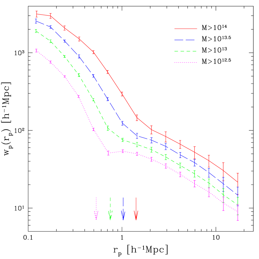
Figure 1.— Projected group-galaxy cross-correlation functions for groups of different mass thresholds. Group masses are estimated from their abundances as described in § 2.2. The mass thresholds are listed in the panel (in units of $h^{-1}M_{\odot}$) and the vertical arrows denote their virial radii. The galaxies used in the cross-correlation have absolute magnitudes $M_{{}^{0.1}\!{r}}<-20$. Errorbars are computed by jackknife resampling of the data set.

3. The Clustering of Groups as a Function of Mass

Figure 1 shows the group-galaxy projected cross-correlation functions for our four mass-threshold group samples. On small scales, this essentially counts pairs between each group center and its member galaxies. The cross-correlation function on these scales thus simply reflects the average radial profile of galaxies within groups. On scales much larger than the typical size of groups, the cross-correlation function counts pairs between groups and galaxies in other groups. The transition between these “1-group” and “2-group” terms (analogous to the 1- and 2-halo terms in the halo model) is striking in Figure 1, much more so than in the galaxy-galaxy autocorrelation function, where it was detected by Zehavi et al. (2004).

Comparing the different group mass samples on small scales, we see that they have cross-correlation functions of very similar shape, but more massive groups have a higher amplitude and are shifted to larger scales than less massive groups. Groups of different masses thus have radial profiles with similar functional forms, but more massive groups contain a higher overall density of galaxies and they extend to larger radii, as expected. The four vertical arrows in Figure 1 show the virial radii of our four mass thresholds, estimated as $R_{\mathrm{vir}}=(3M/800\pi\bar{\rho})^{1/3}$, where $M$ are the thresholds and $\bar{\rho}$ is the mean density of the universe (assuming $\Omega_{m}=0.3$). The 1- to 2-group transitions occur at roughly the virial radii of the mass thresholds, confirming that (1) the location of the transition reflects the typical size of groups being considered, and (2) our estimated group masses yield virial radii that are in agreement with the physical sizes of the groups.

On very small scales ($\lesssim 0.3h^{-1}\mathrm{Mpc}$) the cross-correlation functions flatten, suggesting that the radial profiles of groups have a core. However, on these scales the cross-correlation functions are very sensitive to the definition of group center. Any departure of our estimated centers from the “true” group centers would result in just this sort of flattening.

On large scales, the relative amplitudes of the cross-correlation functions for the different mass groups show that more massive groups are more clustered (i.e., have a higher bias) than less massive groups, as expected. We quantify this dependence in Figure 2, where we show the bias of each sample as a function of its mass threshold (filled black points). We normalize the bias to that for the $\mathrm{log}(M/h^{-1}M_{\odot})>13$ sample and thus compute the bias ratio $b(M)/b(M=10^{13}h^{-1}M_{\odot})$, as described in § 2.3. We obtain errorbars by jackknife resampling of the data on the sky. For comparison, Figure 2 also shows the Seljak & Warren (2004) theoretical bias function of dark matter halos, which we also normalize to $M=13h^{-1}M_{\odot}$ (solid black curve). To first order, our measurements agree with the theory. The large-scale clustering amplitude of groups rises with mass, following the well-known halo bias function (Cole & Kaiser 1989; Mo & White 1996; Sheth & Tormen 1999; Seljak & Warren 2004).

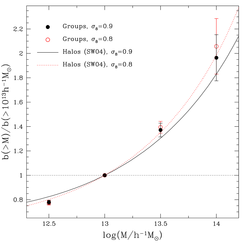
Figure 2.— Large-scale bias of groups as a function of group mass threshold, normalized to the bias of groups with mass greater than $10^{13}h^{-1}M_{\odot}$. Data points are computed by taking the projected galaxy-group cross-correlation function of each group mass sample, dividing by that of the $\mathrm{log}(M/h^{-1}M_{\odot})>13$ sample, and averaging from 5 to 20$h^{-1}\mathrm{Mpc}$. Errorbars show the $1-\sigma$ jackknife uncertainties. The two sets of points show results for group masses estimated using two different cosmological models, as listed in the panel. The two curves show the large-scale bias of dark matter halos as a function of mass (as computed by Seljak & Warren 2004) for the same cosmological models.

In detail, however, Figure 2 shows that the bias function for our groups rises slightly more steeply with mass than the halo bias function $b(M)$. Seljak & Warren (2004) showed that when halo mass is scaled by the nonlinear mass $M_{*}$, the bias function $b(M/M_{*})$ is fairly invariant to the values of cosmological parameters, at least for the limited range of parameter space explored by those authors (deviations from this were shown by Tinker et al. 2005). In other words, most of the effect of changing the cosmological model comes from the corresponding change in $M_{*}$. This means that, in order to have a steeper halo bias function, we must lower $M_{*}$. Lowering $M_{*}$ will make two fixed masses (e.g., $10^{13}$ and $10^{14}h^{-1}M_{\odot}$) move to higher values of $M/M_{*}$, which will yield a steeper bias ratio between the two masses. The cosmological parameter that has the strongest impact on $M_{*}$ is the power spectrum amplitude $\sigma_{8}$, with the mass density $\Omega_{m}$ having a secondary effect and the spectral index $n_{s}$ placing third. The red dotted curve in Figure 2 shows the resulting halo bias function when $\sigma_{8}$ is lowered from 0.9 to 0.8. As expected, the function becomes steeper. In order to be self-consistent, we must now also use this lower value of $\sigma_{8}$ when we assign group masses. Lowering $\sigma_{8}$ decreases the abundance of massive halos, which leads to lower masses for all groups. This, in turn, will make our fixed-mass threshold samples contain fewer and more rare groups (i.e., higher $M/M_{*}$) that are more strongly clustered. We calculate new group masses using $\sigma_{8}=0.8$ and re-make our samples. We show the resulting bias function in Figure 2 (open red points). The observed group bias function becomes slightly steeper, but the change is well within the errorbars and smaller than the corresponding change in the theoretical halo bias curve, especially for our lowest mass sample. The theory now gives a better match to the data.

These results demonstrate that, in principle, the combination of group abundances and clustering (one to get the mass scale and the other to compare to theory) has the power to constrain cosmological parameters (see, e.g., Mo et al. 1996). For example, if we were to take our errors at face value and assume no systematic errors, our data would rule out the $(\Omega_{m},\sigma_{8},n_{s})=(0.3,0.9,1.0)$ model at very high confidence. Moreover, lowering $\Omega_{m}$ to 0.25 or $n_{s}$ to 0.95 would move in the right direction, but would not be sufficient to give good agreement. $\sigma_{8}$ would have to be lowered as well. However, this exercise is not very meaningful without carefully taking into account the main systematic effects present in the analysis: (1) our groups do not perfectly correspond to halos, and (2) we are ignoring the scatter in the luminosity-mass relation when we assign group masses. These issues are especially important given that almost all of the constraining power that we have just discussed comes from our lowest mass sample, where most groups only contain a couple galaxies. Properly addressing our systematic errors would require analysis of realistic mock catalogs constructed using a range of input cosmological parameters, in order to understand the biases resulting from group identification, and it is beyond the scope of this paper. The main thing we wish to take away from Figure 2 is that the bias of our groups agrees with that expected for halos. This acts as a good sanity check that our group samples are not too different from their underlying halos. Furthermore, our data seem to prefer a low value for $M_{*}$, in agreement with current CMB constraints (Spergel et al. 2006), but we cannot say more than this without a detailed treatment of systematic effects.

4. The Clustering of Groups as a Function of Other Properties

We have established that the large-scale clustering of our groups depends on mass in the manner expected of dark matter halos. We now move on to explore the dependence of clustering on other group properties. Since many group properties are likely to correlate with mass, it is possible that any clustering dependence we find is simply due to this correlation. Therefore, it is important that we control for mass and look for residual dependencies on other group properties at fixed mass. For each mass threshold sample and for each group property, we split the groups into a “high” half and a “low” half according to that property, in a way that keeps the mass distributions of the two halves equal.

The properties we consider are:

(a) $(g-r)_{\mathrm{tot}}$ (Total group color): We compute a total color for each group by adding up all the $r$-band light to get $M_{r,\mathrm{tot}}$, adding up all the $g$-band light to get $M_{g,\mathrm{tot}}$, and setting $(g-r)_{\mathrm{tot}}=M_{g,\mathrm{tot}}-M_{r,\mathrm{tot}}$. This is essentially a luminosity-weighted color. Redder groups make it into the “high” samples and bluer groups make it into the “low” samples.

(b) $(g-r)_{\mathrm{cen}}$ (Central galaxy color): We define the central galaxy to be the most luminous in each group (in the $r$-band) and use its ${}^{0.1}\!{(g-r)}$ color. Groups with redder central galaxies make it into the “high” samples and groups with bluer central galaxies make it into the “low” samples.

(c) $(g-r)_{\mathrm{avg}}$ (Average galaxy color): We take the average ${}^{0.1}\!{(g-r)}$ color of all the galaxies in each group. This weights all galaxies equally and thus counts satellite (non-central) galaxies more than the total group color. Again, redder groups make it into the “high” samples and bluer groups make it into the “low” samples.

(d) $M_{r,\mathrm{cen}}$ (Central galaxy luminosity): This is just the absolute $r$-band magnitude of the most luminous galaxy in each group. In cases where $N=1$, $M_{r,\mathrm{cen}}$ is naturally equal to $M_{r,\mathrm{tot}}$. Groups with a more luminous central galaxy make it into the “high” samples and groups with a less luminous central galaxy make it into the “low” samples.

(e) $N$ (Group multiplicity): The number of galaxies with $M_{{}^{0.1}\!{r}}<-19.9$ in each group. We consider all values, from $N=1$ isolated galaxies, to high $N$ rich clusters. Groups with more members make it into the “high” samples and groups with fewer members make it into the “low” samples.

(f) $n_{\mathrm{cen}}$ (Central galaxy concentration): A seeing-convolved Sérsic model is fit to the $i$-band radial light profile (Blanton et al. 2003b). The Sérsic index $n$ is a parameter of the fit and it is a measure of the concentration of the light. $n=1$ and 4 correspond to exponential and de Vaucouleurs profiles, respectively. Values greater than $n\sim 5.9$ are capped at that value. We use the Sérsic index of the most luminous galaxy in each group. Groups with a more concentrated central galaxy make it into the “high” samples and groups with a less concentrated central galaxy make it into the “low” samples.

(g) $\sigma_{v}$ (Group velocity dispersion): This is simply the redshift dispersion of each group, as described in Berlind et al. (2006). Groups with $N=1$ have $\sigma_{v}=0$. Groups with a higher velocity dispersion make it into the “high” samples and groups with a lower velocity dispersion make it into the “low” samples.

(h) $M_{r,\mathrm{2-1}}$ (Luminosity gap): This is the magnitude difference between the first and second most luminous galaxies in each group (in the $r$-band): $M_{r,\mathrm{2-1}}=M_{r,2}-M_{r,\mathrm{cen}}$. In groups with only one galaxy, we use the lower limit for the luminosity gap, which is the magnitude difference between that galaxy and the magnitude limit of our sample: $M_{r,\mathrm{2-1}}(N=1)=19.9-M_{r,\mathrm{cen}}$. Groups with a larger gap make it into the “high” samples and groups with a smaller gap make it into the “low” samples. As described in Berlind et al. (2006), galaxies that do not have measured redshifts due to fiber collisions were included in the galaxy sample and assigned the magnitude and redshift of their nearest neighbor. As a result, in some groups, the first and second most luminous galaxies have the same luminosity. Since we have no information about the luminosity gap in these cases, we randomly place half of them in the “high” samples and the other half in the “low” samples.

As mentioned above, we wish to study the dependence of large-scale clustering on these properties at fixed mass in order to remove any clustering dependence coming from their correlation with mass. We do this as follows: for each candidate group, we define a mass bin of width $\Delta\mathrm{log}M=0.2$ (our results are not sensitive to the choice of bin width) centered on the mass of the group, and we create a list of all groups whose estimated masses lie within the bin. We then rank this list according to a given group property and ask whether our candidate group sits in the top or bottom 50% of the ranked list. If it is in the top 50% we place it into the “high” sample, and if it is in the bottom 50% we place it into the “low” sample. In this way, we create two samples of roughly equal size that have identical mass (total luminosity) distributions, but quite disjoint distributions in the group property used to split them. We do this separately for each of the properties in the above list.

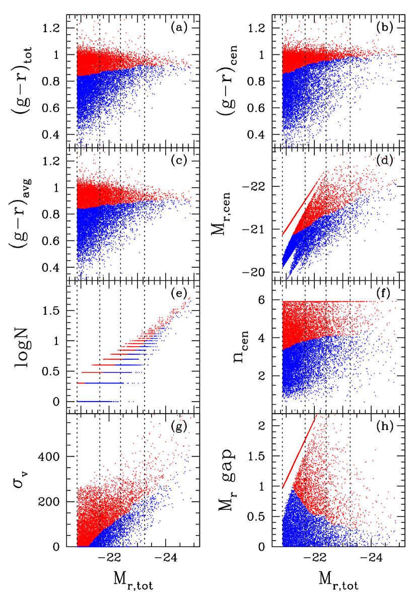
Figure 3.— Group properties as a function of total absolute magnitude, showing the divisions into two samples for each property. Each panel shows a particular group property: (a) total group $g-r$ color, (b) brightest galaxy $g-r$ color, (c) mean galaxy $g-r$ color, (d) brightest galaxy $r$-band absolute magnitude, (e) group multiplicity, (f) brightest galaxy sersic index, (g) group velocity dispersion, (h) absolute magnitude gap between first and second brightest galaxy. For each property, groups are placed into a “top 50%” (red dots) or “bottom 50%” (blue dots) sample depending on whether their value is higher or lower than the median value for all groups at fixed group mass. Vertical dotted lines show the total absolute magnitudes corresponding to our four group mass thresholds.

Figure 3 shows the result of this splitting procedure. Each panel shows the relation between a group property and $M_{r,\mathrm{tot}}$ (our proxy for mass). Groups that were placed in the “high” and “low” samples are represented by red and blue dots, respectively. The four vertical dotted lines show the group luminosities that correspond to our four mass thresholds. The boundary between the two samples in each case shows the median relation of each group property with total group luminosity. Some properties, like central galaxy luminosity, group multiplicity, and velocity dispersion, have strong correlations with group luminosity for all $M_{r,\mathrm{tot}}$, whereas others, such as the three colors, central concentration, and luminosity gap, correlate with group luminosity only at low $M_{r,\mathrm{tot}}$. The three properties that correlate the most with $M_{r,\mathrm{tot}}$ are simple to understand. $M_{r,\mathrm{cen}}$ correlates with $M_{r,\mathrm{tot}}$ because the total group luminosity includes the central galaxy luminosity and is often dominated by it in small groups. At fixed $M_{r,\mathrm{tot}}$, however, we have no reason to think that $M_{r,\mathrm{cen}}$ will correlate with mass. In other words, $M_{r,\mathrm{tot}}$ and $M_{r,\mathrm{cen}}$ probably do not correlate with mass independently of each other. The same is not true for group multiplicity or velocity dispersion. These properties likely correlate with group mass more independently of $M_{r,\mathrm{tot}}$. For example, at fixed group luminosity, groups with higher velocity dispersion probably have larger masses on average than groups with lower velocity dispersion. Another way to say this is that $\sigma_{v}$ and $N$ probably correlate with the scatter in mass at fixed $M_{r,\mathrm{tot}}$.

Now that we have split the groups into halves according to each group property, we can measure the bias ratio $b_{\mathrm{low}}/b_{\mathrm{high}}$ (as described in § 2.3) for each property as a function of group mass. The results are shown in Figure 4. Each type of point corresponds to a particular group property, as listed in the panel. Values of $b_{\mathrm{low}}/b_{\mathrm{high}}$ equal to unity indicate that the large-scale clustering of groups does not depend on that group property. Values above unity indicate that groups in the “low” sample cluster more strongly than those in the “high” sample, and the opposite is true for values below unity.

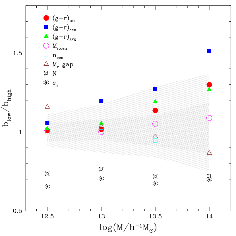
Figure 4.— Ratio of large-scale bias of groups with low values of a given property over that of groups with high values of that property, as a function of group mass threshold. At each mass threshold, different points show this bias ratio for groups split by different properties. Point types and properties are listed in the panel. All points are computed by taking the projected galaxy-group cross-correlation function of the “low” sample, dividing by that of the “high” sample, and averaging from 5 to 20$h^{-1}\mathrm{Mpc}$. The shaded regions enclose 68% (dark shaded region) and 95% (light shaded region) of the values of $b_{\mathrm{low}}/b_{\mathrm{high}}$ that result from randomly splitting the group sample into two halves 200 independent times, and thus represent $1-$ and $2-\sigma$ detection levels.

In order to assess the significance of our results, we create 200 realizations of random “high” and “low” samples, where the group property used in the splitting is a random number. The dark and light shaded regions in Figure 4 enclose 68% and 95% (i.e., $1\sigma$ and $2\sigma$) of these 200 realizations, respectively and are centered on the median. The shaded band grows with mass because the higher mass samples contain fewer groups and their clustering measurements are therefore noisier. We have also computed jackknife errors for our $b_{\mathrm{low}}/b_{\mathrm{high}}$ measurements and verified that they are roughly in agreement with the random splitting errors.

We draw several conclusions from Figure 4:

(1) Only group multiplicity and velocity dispersion correlate significantly with large-scale clustering at all estimated group masses. Furthermore, they behave in exactly the way that is expected if these group properties correlate with mass at fixed group luminosity. Groups with higher $N$ or $\sigma_{v}$ cluster more strongly than groups with lower $N$ or $\sigma_{v}$. Moreover, the bias ratio $b_{\mathrm{low}}/b_{\mathrm{high}}$ is approximately the same ($\sim 0.7$) for both properties and for all masses. If $N$ and $\sigma_{v}$ correlate with mass at fixed group luminosity, as we expect, then their bias ratio will depend on two factors: the amount of scatter in the luminosity-mass relation (after all, if the scatter is zero then $N$ and $\sigma_{v}$ cannot provide additional information on the mass), and the steepness of the bias function $b(M)$ (the steeper the function, the more a given amount of scatter can affect the bias). These two effects have opposite dependencies on mass: as mass increases, the scatter in the luminosity-mass relation should decrease, while the bias function steepens. Figure 4 suggests that these two effects balance each other out to produce a roughly constant $b_{\mathrm{low}}/b_{\mathrm{high}}$ ratio as a function of mass.

(2) The three group colors that we consider show evidence of a correlation with large-scale clustering at high mass, but not at low mass. Of these, the most significant is the central galaxy color. High-mass groups and clusters with blue central galaxies are more strongly biased than those with red central galaxies. Actually, at these masses almost all central galaxies are red (see the second panel in Fig. 3), so it is more accurate to say that groups with less red central galaxies are more clustered than those with redder central galaxies. This is a $\sim 2\sigma$ effect for the $10^{13}$ and $10^{13.5}h^{-1}M_{\odot}$ mass thresholds and grows to a $\sim 3\sigma$ effect at $10^{14}h^{-1}M_{\odot}$. There is a similar effect for total and average group colors in the sense that less red massive groups are more biased than redder groups, but it is only at the $\sim 1.5\sigma$ level of significance. Moreover, group color correlates with central galaxy color by construction, so it is not clear how much of the signal seen for total and average group color actually comes from the color of the central galaxy.

(3) There is a hint that, at high masses, groups with more concentrated central galaxies are more biased than groups with less concentrated central galaxies. This may seem to be in conflict with the result for central galaxy color because usually more concentrated galaxies are redder. However, at these very high luminosities, no such correlation exists. In any case, this is only a $1\sigma$ measurement, so we do not consider it significant.

(4) The luminosity gap statistic shows that groups with smaller gaps are more biased at low masses and less biased at high masses. At high masses this is only a $1\sigma$ effect, but at the lowest mass threshold it is a $\sim 3\sigma$ effect. We must be cautious, however, because at these lowest masses, a large fraction of groups have $N=1$, where the gap statistic is highly unreliable. There could therefore be a large systematic error that affects this point. We test this by repeating the measurement after throwing out all $N=1$ groups, and we find that the detection disappears completely. The overall significance of the luminosity gap detections are therefore low.

(5) Central galaxy luminosity does not appreciably correlate with large-scale clustering at fixed total group luminosity. Since we are comparing samples at fixed total group luminosity, splitting by central galaxy luminosity is the same as splitting by the ratio of central-to-total luminosity. This ratio is similar to the luminosity gap statistic in the sense that groups with a high central-to-total luminosity ratio are likely to also have a large luminosity gap. However, the central-to-total ratio is more robust than the luminosity gap because it is less affected by systematic effects due to incompleteness and group misidentification. The different behavior exhibited by these two statistics provides additional evidence that the luminosity gap results are not significant.

Aside from the observed clustering dependence on group multiplicity and velocity dispersion, which are most likely due to their correlation with mass, our most significant detection is that group color (especially the central galaxy color) correlates with large-scale bias in high luminosity groups. The simplest explanation for this effect is that group color correlates with mass at fixed group luminosity, much like multiplicity and velocity dispersion. One potential problem with this explanation is that the observed bias ratio for central galaxy color is more extreme than that for velocity dispersion, which implies that color must correlate more strongly with mass than does $\sigma_{v}$. This definitely seems odd, but perhaps it is true. Since we know that velocity dispersion should correlate with mass at fixed group luminosity, we can check whether groups with less red central galaxies have a different $\sigma_{v}$ distribution than groups with redder central galaxies.

Figure 5 shows the velocity dispersion distributions for the “high” (solid red histograms) and “low” (dotted blue histograms) samples for each group property in the case of $\mathrm{log}(M/h^{-1}M_{\odot})>14$ groups. Each panel also lists the mean values of $\sigma_{v}$ for the two samples. With the exception of multiplicity and, of course, velocity dispersion itself, all other properties have “high” and “low” samples with nearly identical distributions. In other words, these properties show no correlation with $\sigma_{v}$. This result provides strong evidence that whatever trends exist in Figure 4 are not due to correlations with mass. The one notable exception is group multiplicity, which correlates with $\sigma_{v}$, as expected.

We discuss the implications of these results in § 6.

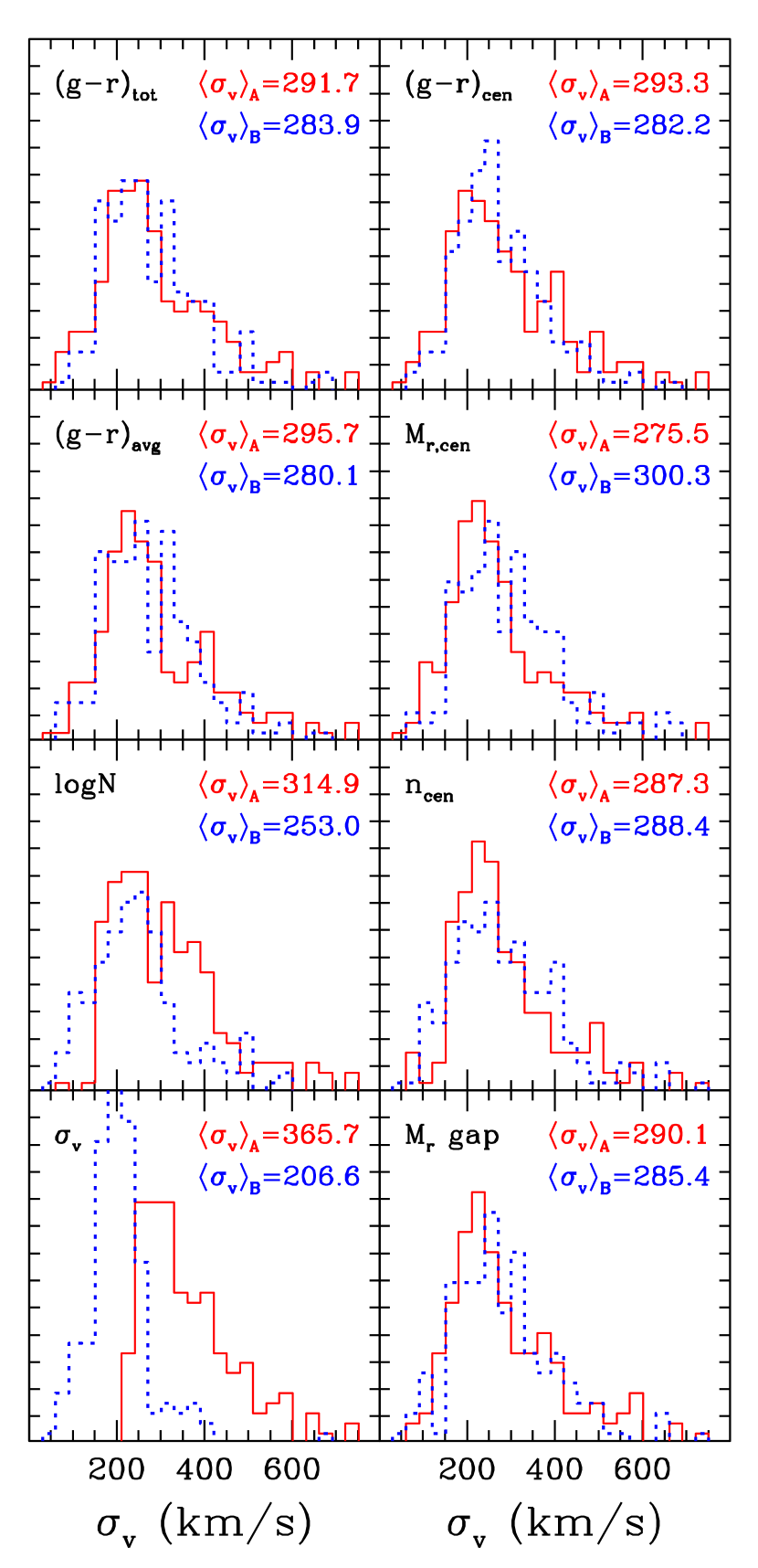
Figure 5.— Velocity dispersion histograms for samples of massive ($M>10^{14}h^{-1}M_{\odot}$) groups split by different group properties. Each panel shows a particular group property, as in Fig. 3. In each panel, the solid and dotted histograms show the velocity dispersion distribution for groups with high and low values of the property, respectively. The mean velocity dispersion for the “high” and “low” samples are denoted $\langle\sigma_{v}\rangle_{A}$ and $\langle\sigma_{v}\rangle_{B}$, respectively, and are listed in each panel.

5. The Clustering of Halos

In the previous section, we showed that there is a significant dependence of high mass group clustering on a group property other than mass, and that this dependence is most likely not due to a correlation with mass. One possibility is that this is a detection of the recently discovered assembly bias for dark matter halos; namely, that halo clustering depends on halo age/concentration at fixed mass. Wechsler et al. (2006) found that for $M>M_{\ast}$, low concentration halos are more strongly biased than high concentration halos. However, the simulations used in that study were fairly small in volume (albeit very high in resolution) making it difficult to study the high mass regime where halos are rare. By necessity, the Wechsler et al. (2006) results for high $M/M_{\ast}$ came from high redshift outputs of the simulation, where $M_{\ast}$ is lower. Wetzel et al. (2006) investigated this with a much larger simulation and confirmed the Wechsler et al. (2006) results for high mass halos.

We wish to compare the age/concentration effect for high mass halos to our results for galaxy groups. We therefore need to know the ratio $b_{\mathrm{low}}/b_{\mathrm{high}}$ for halos, where halos are split into “low” and “high” samples in a similar way as groups were split in § 4. We do this using a set of N-body simulations, which we describe below.

5.1. N-body Simulations and Analysis

We use 20 independent N-body simulations of a $\Lambda$CDM cosmological model, with $\Omega_{m}=0.27$, $\Omega_{\Lambda}=0.73$, $\Omega_{b}=0.046$, $h\equiv H_{0}/(100~{}\mathrm{km~{}s}^{-1}~{}\mathrm{Mpc}^{-1})=0.72$, $n_{s}=1.0$, and $\sigma_{8}=0.9$. Each simulation follows the evolution of $512^{3}$ dark matter particles of mass $m_{p}=7.49\times 10^{10}h^{-1}M_{\odot}$ in a periodic box of length $512h^{-1}\mathrm{Mpc}$. Initial conditions were set up using second-order Lagrangian perturbation theory (2LPT) as described by Crocce et al. (2006), and the simulations were run using the GADGET2 code (Springel 2005). The gravitational force softening was set to $\epsilon_{\rm grav}=40h^{-1}\mathrm{kpc}$ (Plummer equivalent). The simulations are described in more detail in Crocce et al. (2006).

We identify halos in the $z=0$ dark matter particle distributions using a friends-of-friends algorithm with a linking length equal to $0.2$ times the mean inter-particle separation. The mass of each halo is set to the sum of its member particle masses, times a correction factor given by Warren et al. (2006) that accounts for systematic effects due to the finite number of particles per halo. For the large halo masses that we consider in this paper, this correction is never larger than 1.5%. This procedure yields a total of 90231 halos (in all 20 simulations) of mass greater than $10^{14}h^{-1}M_{\odot}$. For each halo, we compute a virial radius equal to $R_{\mathrm{vir}}=\left(\frac{3M}{800\pi\bar{\rho}}\right)^{1/3}$, where $M$ is the halo mass and $\bar{\rho}$ is the mean density of the universe. Finally, we assign center-of-mass coordinates to all halos.

Halo concentrations are simpler to measure than ages because they can be measured from the $z=0$ simulation outputs alone and do not require the construction of merger trees. For this reason, we use concentrations in this study; however, we note that similar results should hold for formation time since these halo properties correlate with each other (Wechsler et al. 2002). We measure a concentration for each halo in the simplest possible way: we choose a fixed fraction of the halo virial radius and measure the ratio of mass enclosed within this radius to the total mass. We choose a value for this fraction equal to 0.3, but we also compute concentrations using values as low as 0.1 and as high as 0.5 in order to test how robust our results are to this definition.

We then split all halos of mass greater than $10^{14}h^{-1}M_{\odot}$ into “high” and “low” samples, in exactly the same way as we split our groups in § 4. For each halo, we create a mass bin of width $\Delta\mathrm{log}M=0.1$ that is centered on that halo’s mass, and we make a list of all halos that lie within this bin. We then sort this list by concentration, and we place the halo in question in the “high” or “low” sample depending on whether its concentration places it in the top or bottom 50% of the sorted list. We also create a second set of samples by choosing halos whose concentrations place them in the top or bottom 25% of halos within their mass bin. In this way, we create halo samples of high and low concentration that have the same mass distributions, thus controlling for the well-known concentration-mass relation (Bullock et al. 2001).

We measure halo-halo autocorrelation functions for the “high” and “low” samples in each of the 20 simulations. We use the simple estimator $\xi(r)=DD/RR-1$, where $DD$ is the number of halo-halo pairs, and $RR$ is the number of random-random pairs, which we calculate analytically as $RR=(1/2)(4/3)\pi\bar{n}^{2}V_{\mathrm{box}}(r_{\mathrm{out}}^{3}-r_{\mathrm{in}}^{3})$, where $\bar{n}$ is the mean density of halos, $V_{\mathrm{box}}$ is the volume of the simulation cube, and $r_{\mathrm{out}}$ and $r_{\mathrm{in}}$ are the outer and inner radii of the bin in which $\xi(r)$ is being calculated. We then calculate bias functions $b(r)=\sqrt{\xi_{\mathrm{low}}(r)/\xi_{\mathrm{high}}(r)}$. We compute average correlation functions and bias functions from the 20 simulations, and we calculate errors from the dispersion among these independent realizations.

5.2. Results

The top panel of Figure 6 shows halo correlation functions for the 50% “low” and “high” samples (thick red curves), as well as the 25% “low” and “high” samples (thin blue curves). All correlation functions show the expected turnover at low scales due to the fact that friends-of-friends halos cannot overlap. There can thus be no halo pairs at separations less than twice the virial radius of the smallest halos considered. The bottom panel shows low/high bias functions for the 50% (thick red curve) and 25% (thin blue curve) samples.

Figure 6 clearly shows that low concentration halos have a significantly higher amplitude of $\xi(r)$ than high concentration halos, at fixed mass. This is a very high signal-to-noise confirmation of the Wechsler et al. (2006) and Wetzel et al. (2006) results. The bias functions become scale-independent at large scales, showing that halo concentration affects the amplitude, but not the shape of the correlation function, as expected. The low/high bias of the 25% samples is naturally higher than that of the 50% samples, but it is interesting that all the difference comes from the high concentration end. The correlation functions of the lowest 50% and 25% concentrated halos have exactly the same amplitude. This means that the relation between concentration and halo bias, at fixed mass, is flat below the median concentration, and only starts dropping at higher concentrations.

We compute large-scale asymptotic values of $b_{\mathrm{low}}/b_{\mathrm{high}}$ by averaging the bias functions in the range where they are scale independent: from 9 to $35h^{-1}\mathrm{Mpc}$. We do this separately for each of the 20 simulations and then compute the mean and uncertainty in the mean, which we calculate from the dispersion among the simulations. The relative bias of low over high concentration halos is $b_{\mathrm{low}}/b_{\mathrm{high}}=1.243\pm 0.017$ for the 50% samples and $b_{\mathrm{low}}/b_{\mathrm{high}}=1.316\pm 0.032$ for the 25% samples. These values are shown in Figure 6 as dotted lines. We note that our results are not sensitive to the specific definition of concentration that we use. When we measure concentrations using different fractions of the virial radius, the values of $b_{\mathrm{low}}/b_{\mathrm{high}}$ change by less than their uncertainties. In the next section, we discuss the connection between these results for halos and those for groups shown in the previous section.

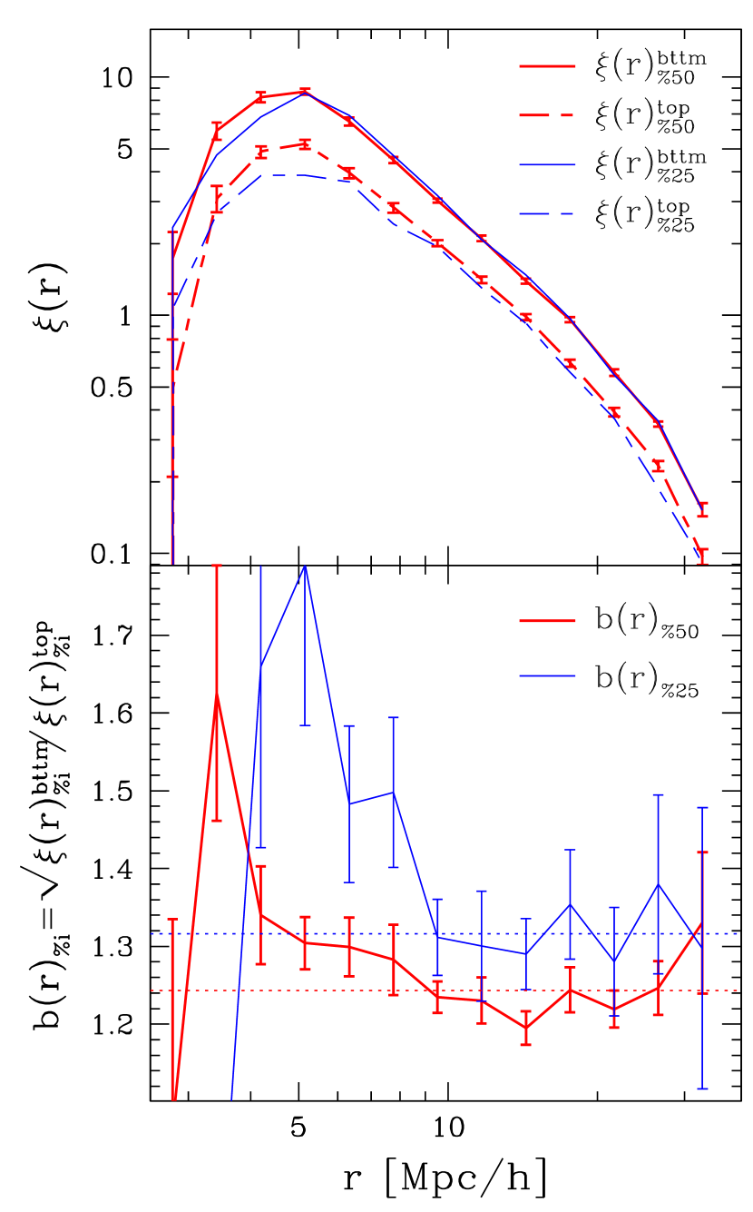
Figure 6.— Top panel: Two-point autocorrelation functions for simulated dark matter halos of mass greater than $10^{14}h^{-1}M_{\odot}$, split into subsamples by concentration. Thick red solid and dashed curves show correlation functions of the 50% least and most concentrated halos, respectively. Thin blue solid and dashed curves show the same for the 25% least and most concentrated halos. Bottom panel: Bias function defined as the square root of the correlation function for low concentration halos divided by that for high concentration halos. The thick red, and thin blue curves shows the bias for the 50% and 25% concentration splits, respectively. Horizontal doted lines show the values of the bias, averaged from 9 to 35$h^{-1}\mathrm{Mpc}$ in these two cases. The values of this large-scale bias are $1.243\pm 0.017$ and $1.316\pm 0.032$ for the 50% and 25% concentration splits, respectively. In both panels, results are averaged over 20 independent N-body simulations, and errors show the uncertainty in the mean estimated from the dispersion among these simulations.

6. Discussion

In § 4, we found that the large-scale bias of massive groups correlates with their central galaxy color, at fixed estimated group mass. Specifically, massive groups with less red central (brightest) galaxies cluster more strongly than those with redder central galaxies. Furthermore, we showed that this trend is probably not due to a correlation of central galaxy color with true mass at fixed estimated mass. In other words, we have found that the large-scale clustering of massive groups depends on a “second parameter” other than mass. This result can be understood in the context of the recent findings by Wechsler et al. (2006) and Wetzel et al. (2006), as well as our results in § 5, showing that massive dark matter halos also have a “second parameter”, whether it be concentration, age, or some other feature of the halo assembly history. If central galaxy color correlates with halo concentration or age at fixed halo mass, then it will also correlate with large-scale bias, since halo concentration and age correlate with bias. Moreover, the effect should only be present at high masses, and should disappear as $M$ approaches $M_{\ast}$, which is exactly what we find. This means that our result for groups most likely constitutes observational evidence for the recently discovered “second parameter” effect for halos. The only alternative is that the color of a halo’s central galaxy somehow “knows” about the density field at large scales ($\sim 10h^{-1}\mathrm{Mpc}$), independently of its halo’s assembly history. Though possible in principle, this is highly unlikely.

For groups of mass greater than $10^{14}h^{-1}M_{\odot}$, we found that the relative bias between groups with the bottom and top 50% of central galaxy color is $b_{\mathrm{low}}/b_{\mathrm{high}}\sim 1.5\pm 0.2$. For comparison, the relative bias between the 50% low and high concentration halos in our simulations is $b_{\mathrm{low}}/b_{\mathrm{high}}=1.243\pm 0.017$. This bias ratio is closer to what we found for total and average group color. This difference could indicate that central galaxy color correlates with a feature of the halo assembly history that is more directly tied to large-scale bias than concentration. However, the difference between these numbers is not highly statistically significant. This highlights the need for repeating these observational investigations with a much larger sample volume that contains a much larger number of massive groups.

Our results imply that massive halos that formed earlier contain redder central galaxies than halos of the same mass that assembled more recently. This is interesting because it is not obvious what one should expect. One could argue that recently assembled halos are more likely to have had a recent major merger, which might result in a central galaxy with no star formation, whereas older halos might contain central galaxies that have had time since their last merger to accrete gas and have some ongoing star formation. On the other hand, one could argue that in this high mass regime, there will be no cool gas to accrete and that older halos will simply have older central galaxy stellar populations. Our results suggest the latter scenario.

It is interesting that the luminosity gap, which we expected to be the group property most directly related to age, showed no significant correlation with large-scale bias at fixed mass. The reasoning behind our expectation is that in old groups, satellite galaxies will have had more time to merge with the central galaxy, resulting in a very massive central galaxy and thus a large luminosity gap. If anything, our results show the opposite trend than expected: massive groups with a high luminosity gap (and hence older) are slightly more clustered than groups with a low gap. This contradicts the theoretical results for halos. One possible explanation for this is that the luminosity gap does not actually correlate with age in the way we expect. However, it could also be that our measured luminosity gaps suffer severely from systematic effects due to incompleteness and group misidentification and are, therefore, not representative of the true luminosity gaps within halos. We believe this latter explanation because we find quite different results when we study the dependence of clustering on central galaxy luminosity, which should act like the luminosity gap. Old groups should have both a larger luminosity gap, and a more luminous central galaxy than young groups of the same mass.

Zentner et al. (2005) predicted that halo concentrations and formation times should be correlated with the number of subhalos within the halo in the sense that older, more concentrated halos have fewer subhalos. This correlation arises because older halos accrete their subhalos earlier and thus give them more time to sink to the center and be destroyed. If this prediction is correct, we should see a trend whereby high mass groups with many member galaxies (high $N$) are more strongly biased than poorer groups of the same mass. Moreover, this trend should disappear at smaller group masses since the bias-age trend also goes away at smaller masses. In this paper, we find the predicted trend at high masses, but, unlike the prediction, it persists at lower masses. It is not straightforward to interpret our result in terms of the Zentner et al. (2005) prediction because we do not compare groups at fixed mass, but rather at fixed total luminosity. If group multiplicity $N$ correlates with group mass at fixed group luminosity then we also expect a trend like the one we find. Since the trend we see persists at low group masses, we conclude that we are likely detecting a multiplicity-mass correlation rather than an intrinsic multiplicity-bias relation.

Yang et al. (2006) have also detected a “second parameter” effect for groups. In a study similar to ours, but using 2dFGRS groups, they found that groups containing central galaxies with low SFR are more biased than groups containing central galaxies with high SFR. Moreover, they found this effect at all group masses. This seems to be at odds with our results because if low SFR implies redder color, then we have found the opposite effect. Yang et al. (2006) use the Madgwick et al. (2002) $\eta$ parameter as a proxy for SFR, which reflects the average emission- and absorption-line strength in the galaxy rest frame spectrum. This is not necessarily correlated with $g-r$ color for the luminous red galaxies that are the central galaxies of these massive systems. Nevertheless, at its face, this result looks completely opposite to ours and remains an interesting puzzle.

7. Summary

In this paper we have investigated the clustering of galaxy groups in the SDSS. The principal goal of this study was to look for secondary dependences of large-scale clustering on group properties other than mass. We have estimated group masses from their abundances using the total group luminosity as a proxy for mass. Our main results are:

1. The measured large-scale bias of groups as a function of estimated mass is in agreement with the theoretical halo bias function, given a standard $\Lambda$CDM cosmological model. The measurements suggest a preference for a low value of $\sigma_{8}$, in agreement with current CMB constraints, but this result is not robust since it could be subject to systematic effects.

2. We have measured the residual dependence of group bias on other group properties, at fixed estimated mass. The properties we have considered are: total group color, central galaxy color, average group color, central galaxy luminosity, group multiplicity (richness), central galaxy concentration, group velocity dispersion, luminosity gap between first and second brightest galaxies. Of these properties, only group multiplicity, velocity dispersion, and central galaxy color show a significant correlation with bias at fixed estimated mass. Specifically, groups with higher multiplicity, higher velocity dispersion, and less red central galaxies cluster more strongly than groups with the opposite properties. The effect for multiplicity and velocity dispersion occurs at all masses, whereas the effect for central galaxy color is only significant at high group masses ($M>10^{14}h^{-1}M_{\odot}$).

3. The dependence of large-scale bias on group multiplicity and velocity dispersion can be simply explained if these properties correlate with true mass at fixed estimated mass. However, the dependence of bias on central galaxy color cannot be explained this way and is most likely a real effect. This is likely observational evidence of recent theoretical findings that halo bias depends on a “second parameter” other than mass, such as age or concentration.

4. Our results imply a connection between halo age and central galaxy color for massive halos. Halos that assembled earlier likely contain redder central galaxies than recently assembled halos of the same mass.

5. In order to compare our results to theory, we have quantified the dependence of halo bias on concentration for high mass halos, using a set of large N-body simulations. We find that low concentration halos are more biased on large scales than high concentration halos, at fixed mass, thus confirming previous results at very high signal-to-noise. Specifically, we find that for halos with $M>10^{14}h^{-1}M_{\odot}$, the relative bias between the 50% least and most concentrated halos is $b_{\mathrm{low}}/b_{\mathrm{high}}=1.243\pm 0.017$, while the relative bias between the 25% least and most concentrated halos is $b_{\mathrm{low}}/b_{\mathrm{high}}=1.316\pm 0.032$.

References

- Abbas & Sheth (2006) Abbas, U., & Sheth, R. K. 2006, ArXiv Astrophysics e-prints
- Adelman-McCarthy et al. (2006) Adelman-McCarthy, J. K. et al. 2006, ApJS, 162, 38
- Bahcall et al. (2003) Bahcall, N. A., Dong, F., Hao, L., Bode, P., Annis, J., Gunn, J. E., & Schneider, D. P. 2003, ApJ, 599, 814
- Bahcall & Soneira (1983) Bahcall, N. A., & Soneira, R. M. 1983, ApJ, 270, 20
- Berlind et al. (2006) Berlind, A. A. et al. 2006, ArXiv Astrophysics e-prints
- Berlind & Weinberg (2002) Berlind, A. A., & Weinberg, D. H. 2002, ApJ, 575, 587
- Blanton & Berlind (2006) Blanton, M. R., & Berlind, A. A. 2006, ArXiv Astrophysics e-prints
- Blanton et al. (2003a) Blanton, M. R. et al. 2003a, AJ, 125, 2348
- Blanton et al. (2003b) —. 2003b, ApJ, 594, 186
- Blanton et al. (2003c) —. 2003c, ApJ, 592, 819
- Blanton et al. (2003d) Blanton, M. R., Lin, H., Lupton, R. H., Maley, F. M., Young, N., Zehavi, I., & Loveday, J. 2003d, AJ, 125, 2276
- Blanton et al. (2005) Blanton, M. R. et al. 2005, AJ, 129, 2562
- Bullock et al. (2001) Bullock, J. S., Kolatt, T. S., Sigad, Y., Somerville, R. S., Kravtsov, A. V., Klypin, A. A., Primack, J. R., & Dekel, A. 2001, MNRAS, 321, 559
- Coil et al. (2006) Coil, A. L. et al. 2006, ApJ, 638, 668
- Cole & Kaiser (1989) Cole, S., & Kaiser, N. 1989, MNRAS, 237, 1127
- Colless et al. (2001) Colless, M. et al. 2001, MNRAS, 328, 1039
- Cooray & Sheth (2002) Cooray, A., & Sheth, R. 2002, Phys. Rep., 372, 1
- Crocce et al. (2006) Crocce, M., Pueblas, S., & Scoccimarro, R. 2006, ArXiv Astrophysics e-prints
- Croton et al. (2006) Croton, D. J., Gao, L., & White, S. D. M. 2006, ArXiv Astrophysics e-prints
- Davis & Peebles (1983) Davis, M., & Peebles, P. J. E. 1983, ApJ, 267, 465
- Eisenstein et al. (2001) Eisenstein, D. J. et al. 2001, AJ, 122, 2267
- Fisher et al. (1994) Fisher, K. B., Davis, M., Strauss, M. A., Yahil, A., & Huchra, J. 1994, MNRAS, 266, 50
- Fukugita et al. (1996) Fukugita, M., Ichikawa, T., Gunn, J. E., Doi, M., Shimasaku, K., & Schneider, D. P. 1996, AJ, 111, 1748
- Gao et al. (2005) Gao, L., Springel, V., & White, S. D. M. 2005, MNRAS, 363, L66
- Geller & Huchra (1983) Geller, M. J., & Huchra, J. P. 1983, ApJS, 52, 61
- Giuricin et al. (2000) Giuricin, G., Samurovic, S., Girardi, M., Mezzetti, M., & Marinoni, C. 2000, in Constructing the Universe with Clusters of Galaxies
- Gunn et al. (1998) Gunn, J. E. et al. 1998, AJ, 116, 3040
- Gunn et al. (2006) —. 2006, AJ, 131, 2332
- Harker et al. (2006) Harker, G., Cole, S., Helly, J., Frenk, C., & Jenkins, A. 2006, MNRAS, 367, 1039
- Hogg et al. (2001) Hogg, D. W., Finkbeiner, D. P., Schlegel, D. J., & Gunn, J. E. 2001, AJ, 122, 2129
- Ivezić et al. (2004) Ivezić, Ž. et al. 2004, Astronomische Nachrichten, 325, 583
- Landy & Szalay (1993) Landy, S. D., & Szalay, A. S. 1993, ApJ, 412, 64
- Lupton (2005) Lupton, R. H. 2005, AJ, submitted
- Lupton et al. (2001) Lupton, R. H., Gunn, J. E., Ivezić, Z., Knapp, G. R., Kent, S., & Yasuda, N. 2001, in ASP Conf. Ser. 238: Astronomical Data Analysis Software and Systems X, 269–+
- Madgwick et al. (2002) Madgwick, D. S. et al. 2002, MNRAS, 333, 133
- Mo et al. (1996) Mo, H. J., Jing, Y. P., & White, S. D. M. 1996, MNRAS, 282, 1096
- Mo & White (1996) Mo, H. J., & White, S. D. M. 1996, MNRAS, 282, 347
- Padilla et al. (2004) Padilla, N. D. et al. 2004, MNRAS, 352, 211
- Peacock & Smith (2000) Peacock, J. A., & Smith, R. E. 2000, MNRAS, 318, 1144
- Pier et al. (2003) Pier, J. R., Munn, J. A., Hindsley, R. B., Hennessy, G. S., Kent, S. M., Lupton, R. H., & Ivezić, Ž. 2003, AJ, 125, 1559
- Richards et al. (2002) Richards, G. T. et al. 2002, AJ, 123, 2945
- Schlegel et al. (1998) Schlegel, D. J., Finkbeiner, D. P., & Davis, M. 1998, ApJ, 500, 525
- Scoccimarro et al. (2001) Scoccimarro, R., Sheth, R. K., Hui, L., & Jain, B. 2001, ApJ, 546, 20
- Seljak (2000) Seljak, U. 2000, MNRAS, 318, 203
- Seljak & Warren (2004) Seljak, U., & Warren, M. S. 2004, MNRAS, 355, 129
- Sheth & Tormen (1999) Sheth, R. K., & Tormen, G. 1999, MNRAS, 308, 119
- Sheth & Tormen (2004) —. 2004, MNRAS, 350, 1385
- Skibba et al. (2006) Skibba, R., Sheth, R. K., Connolly, A. J., & Scranton, R. 2006, MNRAS, 369, 68
- Smith et al. (2002) Smith, J. A. et al. 2002, AJ, 123, 2121
- Spergel et al. (2006) Spergel, D. N. et al. 2006, ArXiv Astrophysics e-prints
- Springel (2005) Springel, V. 2005, MNRAS, 364, 1105
- Springel et al. (2005) Springel, V. et al. 2005, Nature, 435, 629
- Strauss et al. (2002) Strauss, M. A. et al. 2002, AJ, 124, 1810
- Tinker et al. (2005) Tinker, J. L., Weinberg, D. H., Zheng, Z., & Zehavi, I. 2005, ApJ, 631, 41
- Tucker et al. (2006) Tucker, D. L. et al. 2006, Astronomische Nachrichten, 327, 821
- Warren et al. (2006) Warren, M. S., Abazajian, K., Holz, D. E., & Teodoro, L. 2006, ApJ, 646, 881
- Wechsler et al. (2002) Wechsler, R. H., Bullock, J. S., Primack, J. R., Kravtsov, A. V., & Dekel, A. 2002, ApJ, 568, 52
- Wechsler et al. (2006) Wechsler, R. H., Zentner, A. R., Bullock, J. S., Kravtsov, A. V., & Allgood, B. 2006, ApJ, in press
- Wetzel et al. (2006) Wetzel, A. R., Cohn, J. D., White, M., Holz, D. E., & Warren, M. S. 2006, ArXiv Astrophysics e-prints
- Yang et al. (2006) Yang, X., Mo, H. J., & van den Bosch, F. C. 2006, ApJ, 638, L55
- Yang et al. (2005) Yang, X., Mo, H. J., van den Bosch, F. C., & Jing, Y. P. 2005, MNRAS, 357, 608
- York et al. (2000) York, D. G. et al. 2000, AJ, 120, 1579
- Zehavi et al. (2002) Zehavi, I. et al. 2002, ApJ, 571, 172
- Zehavi et al. (2004) —. 2004, ApJ, 608, 16
- Zehavi et al. (2005) —. 2005, ApJ, 630, 1
- Zentner et al. (2005) Zentner, A. R., Berlind, A. A., Bullock, J. S., Kravtsov, A. V., & Wechsler, R. H. 2005, ApJ, 624, 505