We study a class of generalized inflation models in which the inflaton is coupled to the Ricci scalar by a general $f(\varphi,R)$ term. The scalar power spectrum, the spectral index, the running of the spectral index, the tensor mode spectrum and a new consistency relation of the model are calculated. We discuss in detail the issues of how to diagonize the coupled perturbation equations, how to deal with an entropy-like source, and how to determine the initial condition by quantization. By studying some explicit models, we find that rich phenomena such as a blue scalar power spectrum, a large running of the spectral index, and a blue tensor mode spectrum can be obtained.

1 Introduction

Inflation [1] has been very successful in solving the problems in the standard big bang cosmology such as the horizon and flatness problems. Fluctuations are created during inflation, which provide seeds of large scale structure and the Cosmic Microwave Background (CMB) anisotropies having been observed by COBE and WMAP satellites, the latter will be measured more precisely by PLANCK.

In spite of the remarkable achievements, there are still open problems, such as a natural realization of inflation models in a fundamental theory, and how to further pin down a specific model including the number of the inflatons and the form of the potential. In ref.[2], some theoretical problems are listed. For example, the hierarchy of scales, the trans-Planck problem, the singularity problem and the candidate of the inflaton. As for the data fitting, there is still a significant power deficit at $l=2$, and if the running of the spectral index is introduced as a parameter, the WMAP three year data mildly favors a blue spectrum with a large running [3], which is not common in inflation models. In the past, a few models were proposed to accommodate a large negative running such as the noncommutative inflation model [4]. For other models we refer to [5, 6, 7, 8]. Discussions on models violating the null energy condition and leading to a blue tensor spectrum and possibly a blue scalar spectrum, as well as on the WMAP three year constraints, can be found in [9]

To have a broad scope, and to be prepared for possible surprises in the future experiments, it is essential to study classes of models with novel physics built in, for example, quantum gravity and string theory may induce higher derivative corrections. In this paper, our primary goal is to carry out a more careful study of a class of models in which in addition to the Hilbert-Einstein action and a minimal coupled inflaton, there is a general nominimal coupling of the form $f(\varphi,R)$. Some of these models were studied before. However, when we examined the literature carefully, we found that only some special models were reliably studied. These include: $f(R)$ gravity models [11] and the $f(\varphi)R$ gravity models [12], a unified analysis of these two cases were made in [13]. Furthermore, even for $f(R)$ action and $f(\varphi)R$ action, no concrete models were investigated in detail. Remarkably, the result for the tensor modes power spectrum in [13] is applicable to more general cases. We note, however, that the pioneering work on inflation with an additional scalar curvature squared term was done long time ago [10]

In [14], the models with a nonminimal coupling term $-\frac{1}{2}f(\frac{1}{6}R)\varphi^{2}$ are studied, and the calculations are carried out when $f$ is quadratic in $R$ and the nonminimal coupling gives dominate contribution in the rolling of $\varphi$. It is shown that a blue spectrum with a running larger than that of a common minimal model can be produced. However, the constraints on the fluctuation of the inflaton and the scalar fluctuations in the metric are over-simplified in [14].

In this paper, we study a general class of models in which the coupling between the inflaton $\varphi$ and the Ricci scalar $R$ is described by a general function $f(\varphi,R)$. Both the background dynamics and the perturbations are studied, and the power spectrum, the spectral index, the running of the spectral index and the perturbations for the tensor modes are calculated, which can be related to the experiments today and in the future.

Some ingredients in the calculations are standard as being used in the minimal inflation models ([15] is a nice review). Due to the higher derivative terms, the constraints among the fluctuations are no longer purely algebraic. We develop a general method to deal with this problem. Diagonalization of the perturbation equations is no longer simple. Upon assuming a slow-roll inflation, we can still have a nearly-conserved quantity which reduces to the usual curvature perturbation when the higher derivative terms are suppressed. Thus, although there is an entropy-like perturbation, we can bypass this problem by using this new nearly-conserved quantity. Also, since we can not directly write down the action for the perturbation modes, we provide an argument in relating the perturbation in a diagonalized perturbation equation to the canonically normalized mode, thus set the initial quantization condition. Some of these methods are quite general and can be used in other generalizations of the minimal inflation models.

By calculating the power spectrum and related quantities, we find that there are rich phenomena in this class of models. We can have a blue spectrum and a large running of the spectral index in some models, while in other models the spectrum stay red and the running can become positive. Also, in principle, one can have an initial fast-rolling period when the higher derivative terms are comparable to the Hilbert-Einstein term. The consistency condition between $r$ and $n_{T}$ is modified. A blue tensor mode power spectrum can appear even in some small inflaton models in some parameter region while in minimal inflation models the tensor spectrum is always red.

The paper is organized as follows. In Section 2, we derive the equations of motion of background quantities, and spell out the conditions of slow-roll approximation. In Section 3, we write down the equations for perturbations. After diagonalizing and simplifying the equations to obtain a Bessel equation, we propose a nearly-conserved quantity which has the form of comoving curvature perturbation in the minimal inflation model limit. In Section 4, we study the initial conditions by relating the fluctuation under study to the canonically normalized mode. Since the canonical variables are normalized by quantization, this procedure help us to fix the integration constants in the solutions of the Bessel equation. In Section 5, the power spectrum, the spectral index, the running of the spectral index, and the ratio of the tensor and scalar perturbations are given. In Section 6, we calculate several classes of models and discuss the properties of these models. We conclude in Section 7.

2 The Model and Background Dynamics

We consider the following action with nonminimal coupling:

$$S=\int d^{4}x\sqrt{-g}[\frac{1}{2}f(\varphi,R)-\frac{1}{2}g^{\alpha\beta}\partial_{\alpha}\varphi\partial_{\beta}\varphi-V(\varphi)],$$ (1)

We consider first the evolution of the background, a homogeneous and isotropic spacetime with a space-independent inflation field. We work with the Friedmann-Robertson-Walker(FRW) metric

$$ds^{2}=-dt^{2}+a^{2}(t)dx^{2}=a^{2}(\tau)(-d\tau^{2}+dx^{2}),$$ (2)

where $t$ is the comoving time and $\tau$ is the conformal time.

It follows from the action (1) that, the equations of motion are

$$H^{2}=\frac{1}{3M_{p}^{2}}\rho,\leavevmode\nobreak\ \leavevmode\nobreak\ \dot{H}=-\frac{1}{2M_{p}^{2}}(\rho+p),$$ (3)

$$\ddot{\varphi}+3H\dot{\varphi}+\frac{1}{2}(-f_{,\varphi}+2V_{,\varphi})=0,$$ (4)

where $\rho$ and $p$ are energy density and pressure respectively, as the diagonal elements of the spacial averaged energy-momentum tensor, and can be written as

$$\rho = \frac{M_{p}^{2}}{F}(\frac{1}{2}\dot{\varphi}^{2}+V+\frac{RF-f}{2}-3H\dot{F}),$$ (5)

$$p = \frac{M_{p}^{2}}{F}(\frac{1}{2}\dot{\varphi}^{2}-V-\frac{RF-f}{2}+\ddot{F}+2H\dot{F}),$$ (6)

where $F=\frac{\partial}{\partial R}f(\varphi,R)$, and dot denotes the derivative with respect to $t$.

We shall impose the following slow-roll conditions:

$$\epsilon \equiv -\frac{\dot{H}}{H^{2}}\ll 1,$$ (7)

$$\delta \equiv -\frac{\ddot{\varphi}}{H\dot{\varphi}}\ll 1,$$ (8)

$$\gamma \equiv \frac{\dot{F}}{HF}\ll 1,$$ (9)

The first and second slow-roll conditions are standard as in the minimal inflation model. The third slow-roll condition is new in the nonminimal model. It is a natural requirement, because $F$ can be written as a function of $R$ and $\varphi$ and should be slow-rolling during inflation. Moreover, it will be shown that $\gamma$ appears in the spectral index and the ratio of tensor and scalar perturbations. To be consistent with the CMB data, it should be small in any viable candidate inflation model. In addition to the above slow-roll conditions, we further require that the above slow-roll parameters themselves are rolling slowly.

3 Classical Evolution of Perturbations

To calculate the scalar fluctuations, we need to perturb the Einstein equations. Through out the calculations, we will work in the longitudinal gauge,

$$ds^{2}=a^{2}\left(-(1+2\phi)d\tau^{2}+(1-2\psi)dx^{i}dx^{i}\right),$$ (10)

and the fluctuation of the inflaton $\varphi$ is denoted by $\delta\varphi$.

The perturbation equations are

$$3H(H\phi+\dot{\psi})-\frac{1}{a^{2}}\nabla^{2}\psi=-\frac{1}{2M_{p}^{2}}\delta\rho,$$ (11)

$$3(H\phi+\dot{\psi})=\frac{3}{2M_{p}^{2}}(\rho+p)v,$$ (12)

$$\psi-\phi=\frac{\delta F}{F},$$ (13)

$$\ddot{\psi}+3H(H\phi+\dot{\psi})+H\dot{\phi}+2\dot{H}\phi+\frac{1}{3a^{2}}\nabla^{2}(\phi-\psi)=\frac{1}{2M_{p}^{2}}\delta p,$$ (14)

which follow from the components $G^{0}_{0},G^{0}_{j},G^{i}_{j}(i\neq j)$, $G^{i}_{i}$ of the linearized Einstein equations for perturbations, respectively. The $\delta\rho$, $\delta p$ and $v$ are perturbative quantities in the energy momentum tensor defined as,

$$T^{0}_{0}=-(\rho+\delta\rho),\hskip 12.91663ptT^{0}_{i}=-(\rho+p)v_{,i},\hskip 12.91663ptT^{i}_{i}=3(p+\delta p),$$ (15)

with the explicit form

$$\delta\rho = \frac{M_{p}^{2}}{F}[\dot{\varphi}\delta\dot{\varphi}+\frac{1}{2}(-f_{,\varphi}+2V_{,\varphi})\delta\varphi-3H\delta\dot{F}+(3\dot{H}+3H^{2}+\frac{1}{a^{2}}\nabla^{2})\delta F$$ (16)

$$+(3H\dot{F}-\dot{\varphi}^{2})\phi+3\dot{F}(H\phi+\dot{\psi})],$$

$$\delta p = \frac{M_{p}^{2}}{F}[\dot{\varphi}\delta\dot{\varphi}+\frac{1}{2}(f_{,\varphi}-2V_{,\varphi})\delta\varphi+\delta\ddot{F}+2H\delta\dot{F}+(-\dot{H}-3H^{2}-\frac{2}{3a^{2}}\nabla^{2})\delta F$$ (17)

$$-\dot{F}\dot{\phi}-(\dot{\varphi}^{2}+2\ddot{F}+2H\dot{F})\phi-2\dot{F}(H\phi+\dot{\psi})],$$

$$(\rho+p)v = \frac{M_{p}^{2}}{F}(\dot{\varphi}\delta\varphi+\delta\dot{F}-H\delta F-\dot{F}\phi)$$ (18)

By using equations (12) and (13) to cancel $\delta\varphi$ and $\delta F$ terms in (11) respectively, one gets

$$F(\ddot{\phi}+\ddot{\psi})+(HF+3\dot{F}-\frac{2F\ddot{\varphi}}{\dot{\varphi}})(\dot{\phi}+\dot{\psi})$$

$$+[(3H\dot{F}+3\ddot{F})-\frac{2\ddot{\varphi}}{\dot{\varphi}}(HF+2\dot{F})-\frac{F}{a^{2}}\nabla^{2}]\phi$$

$$+[(4\dot{H}F+H\dot{F}-\ddot{F})-\frac{2\ddot{\varphi}}{\dot{\varphi}}(HF-\dot{F})-\frac{F}{a^{2}}\nabla^{2}]\psi=0$$ (19)

And by using $\delta F=F_{,R}\delta R+F_{,\varphi}\delta\varphi$ and $\dot{F}=F_{,R}\dot{R}+F_{,\varphi}\dot{\varphi}$, we can write (13) in a more explicit form

$$F(2\dot{H}F-H\dot{F}+\ddot{F})(\phi-\psi)$$

$$+[6F_{,R}(4H\dot{H}+\ddot{H})-\dot{F}][F(\dot{\phi}+\dot{\psi})+(HF+2\dot{F})\phi+(HF-\dot{F})\psi]=$$

$$2F_{,R}(2\dot{H}F-H\dot{F}+\ddot{F})\times$$

$$[3\ddot{\psi}+3H\dot{\phi}+12H\dot{\psi}+6(2H^{2}+\dot{H})\phi+\frac{1}{a^{2}}\nabla^{2}(\phi-2\psi)]$$ (20)

In the limit of minimal inflation model, (20) reduces to the constraint equation $\psi=\phi$.

Equations (19) and (20) are coupled differential equations for $\psi$ and $\phi$. In some special cases, for example, $F=F(\varphi)$ or $F=F(R)$, these equations can be diagonalized to a single differential equation [13]. While in a more general case which is of main interest in this paper, we have to develop a new method to solve these equations.

To diagonize the equations, we define

$${\cal G}_{k}\equiv\psi_{k}/\phi_{k},$$ (21)

where $\psi_{k}$ and $\phi_{k}$ are Fourier components of $\psi$ and $\phi$, and the explicit $k$-dependence of ${\cal G}_{k}$ will be shown later in this section. We can Taylor expand ${\cal G}_{k}$ as

$${\cal G}_{k}=G_{0}+\frac{F_{,R}H^{2}}{F}\left(\frac{k}{aH}\right)^{2}G_{1}+\cdots,$$ (22)

where $G_{0}$ and $G_{1}$ stand for the zeroth and first coefficients in the Taylor expansion.

So under the condition that the nonminimal coupling is not too strong compared with the minimal coupling gravity, the above expansion works well near the horizon-crossing and we will see in the following sections that $G_{0}$ will be the dominant contribution. It ought to be true for physically interesting models where the energy scale of inflation is smaller than the Planck scale or the string scale. While when the expansion does not work well and the high order terms of $k$ become important, the high order derivative corrections will play a much more important role at the Hubble scale. In this case the dispersion relation will be modified significantly when the perturbation was created, and we need to modify the usually canonical quantization. A quantum gravity theory perhaps is in demand in order to fully understand this regime.

We now derive ${\cal G}_{k}$ as a function of background quantities from (19) and (20). Substitute (21) into (19) and (20) to eliminate $\psi_{k}$, then use (19) and (20) to eliminate the $\phi{{}^{\prime\prime}}$ terms to get a first-order differential equation. Differentiate this equation once and subtract with (19), we can get another first-order differential equation. From the consistence condition of the two first-order differential equations, we can get the expression of ${\cal G}_{k}$, which to the lowest order is the solution of the following equation:

$$\{[F\dot{F}+24HF_{,R}(\dot{H}F-H\dot{F})]{\cal G}_{k}+F(\dot{F}-24H\dot{H}F_{,R})\}$$ (23)

$$\times\{[2H\dot{H}F(F-12H^{2}F_{,R})-4HF_{,R}(4\dot{H}F-5H\dot{F})\frac{k^{2}}{a^{2}}-F\dot{F}\frac{k^{2}}{a^{2}}]{\cal G}_{k}$$

$$-2H(F-12H^{2}F_{,R})(\dot{H}F-H\dot{F})+8HF_{,R}(\dot{H}F+H\dot{F})\frac{k^{2}}{a^{2}}-F\dot{F}\frac{k^{2}}{a^{2}}\}$$

$$= \{[2\dot{H}F(F-12H^{2}F_{,R})-2F_{,R}(2\dot{H}F-H\dot{F})\frac{k^{2}}{a^{2}}]{\cal G}_{k}$$

$$-2(F-12H^{2}F_{,R})(\dot{H}F-H\dot{F})-2F_{,R}(2\dot{H}F-H\dot{F})\frac{k^{2}}{a^{2}}\}^{2},$$

we see that indeed ${\cal G}_{k}$ is a function of only the background. By solving $G_{0}$ and $G_{1}$ from this equation, it can be shown that $G_{0}$ and $G_{1}$ are slow-roll quantities and $G_{0}$ has the simple form

$$G_{0}=1-\frac{\dot{F}H}{F\dot{H}}$$ (24)

With the use of the linear relation between $\psi_{k}$ and $\phi_{k}$, to leading order of slow-roll parameters, we derive a differential equation for a single variable, say $\phi_{k}$

$$\phi{{}^{\prime\prime}}_{k}+(aH)\left(\frac{2\dot{\cal G}_{k}}{H(1+{\cal G}_{k})}+2\delta+3\gamma\right)\phi^{\prime}_{k}+k^{2}\phi_{k}$$

$$+(aH)^{2}\left(\frac{\ddot{{\cal G}_{k}}}{H^{2}(1+{\cal G}_{k})}+\frac{\dot{{\cal G}_{k}}}{H(1+{\cal G}_{k})}-\frac{4{\cal G}_{k}}{1+{\cal G}_{k}}\epsilon+\frac{3+{\cal G}_{k}}{1+{\cal G}_{k}}\gamma+2\delta\right)\phi_{k}=0$$ (25)

By introducing a new variable

$$u_{k}\equiv\frac{F^{\frac{3}{2}}(1+{\cal G}_{k})}{\dot{\varphi}}\phi_{k},$$ (26)

the equation (25) can be rewritten as

$$u{{}^{\prime\prime}}_{k}+\frac{1}{\tau^{2}}\left(\delta+\frac{3-{\cal G}_{k}}{2(1+{\cal G}_{k})}\gamma-\frac{4{\cal G}_{k}}{1+{\cal G}_{k}}\epsilon\right)u_{k}+k^{2}u_{k}=0,$$ (27)

where $(aH)^{2}$ has been replaced by $1/\tau^{2}$ up to the leading order precision.

Inserting the Taylor expansion of ${\cal G}_{k}$, one finds

$$u{{}^{\prime\prime}}_{k}+\frac{1}{\tau^{2}}\left(\delta+\frac{3-G_{0}}{2(1+G_{0})}\gamma-\frac{4G_{0}}{1+G_{0}}\epsilon\right)u_{k}+\tilde{k}^{2}u_{k}=0,$$ (28)

where $\tilde{k}$ is a rescaling of $k$, due to the contribution of the $k$-dependent part of ${\cal G}_{k}$,

$$\frac{\tilde{k}^{2}}{k^{2}}=1+\left(\frac{4G_{0}}{2(1+G_{0})^{2}}\gamma-\frac{4(1+2G_{0})}{(1+G_{0})^{2}}\epsilon\right)\frac{F_{,R}H^{2}}{F}G_{1}$$ (29)

It can be shown in the models under consideration and to the desired precision, this rescaling can be neglected, and we shall use $k$ instead of $\tilde{k}$. If one wish to calculate to second order in slow-roll parameters in this nonminimal model, this rescaling should be taken into account. This effect may also arise in models other than (1).

The equation (28) can be further simplified to

$$u{{}^{\prime\prime}}_{k}+\frac{1}{2\tau^{2}}\left(-4\epsilon+2\delta-\gamma\right)u_{k}+\tilde{k}^{2}u_{k}=0,$$ (30)

Which takes the form of a Bessel equation. The solution of (30) can be written as

$$u_{k}=C_{1}\sqrt{-\tau}H^{(1)}_{\nu}(-k\tau)+C_{2}\sqrt{-\tau}H^{(2)}_{\nu}(-k\tau),$$ (31)

where $C_{1}$ and $C_{2}$ are the integration constants to be determined by the initial conditions, and $\nu$ is

$$\nu\equiv\frac{1}{2}\sqrt{1-2\left(-4\epsilon+2\delta-\gamma\right)}\simeq\frac{1}{2}-\frac{1}{2}(-4\epsilon+2\delta-\gamma)$$ (32)

There are rich phenomenona as preheating and reheating for the perturbations from crossing the horizon to reentering the horizon. In order not to track the whole evolution process, we need to find a conserved quantity well outside the horizon. In the minimal inflation models, the comoving curvature perturbation is introduced to deal with this problem. But in the models with entropy perturbation, the comoving curvature perturbation and its direct generalizations may not be conserved. In this paper, we develop a general method to derive a nearly conserved quantity, which can come back to the form of comoving curvature perturbation in the limit where the physical wave-length is large enough to ignore nonminimal coupling corrections.

In our model, the nearly conserved quantity takes the form

$$\mathcal{R}_{k}\equiv\frac{H}{\dot{H}}\dot{\phi}_{k}+\left(\frac{H^{2}}{\dot{H}}+2\frac{\dot{F}}{F}\frac{H}{\dot{H}}+\frac{\dot{G_{0}}}{1+G_{0}}\frac{H}{\dot{H}}-1\right)\phi_{k}$$ (33)

It can be examined that $\dot{\mathcal{R}_{k}}/(H\mathcal{R}_{k})\sim\mathcal{O}(\epsilon^{2})$. The detailed derivation of this quantity is presented in Appendix A. The issues on entropy perturbation and the differences between the comoving curvature perturbation and the newly-derived quantity are discussed in Appendix B. Since the nearly conserved quantity turns smoothly into the comoving curvature perturbation at late time during inflation, the observables like the temperature fluctuations on the large-angular scales can be directly related to this quantity. The amplitude of entropy perturbation automatically decays well outside the horizon, so it does not conflict with the experiments on the observed limits of entropy perturbations.

4 Quantum Theory of Perturbations

Quantization plays an essential role in creating the perturbations from an initial “vacuum” state, and sets the initial conditions for the solutions to the perturbation equations. To do quantization, we have to expand the action up to second order in the perturbation variables:

$$\delta_{2}S=\frac{1}{2}\int\left((v^{\prime})^{2}-(\partial_{i}v)^{2}+\frac{z{{}^{\prime\prime}}}{z}v^{2}\right)d^{4}x$$ (34)

As usual the commutation relations on the constant conformal time hypersurface are satified by the canonical coordinate $v$ and its conjugate momentum.

The equation of motion of $v$ takes the form:

$$v{{}^{\prime\prime}}_{k}+k^{2}v_{k}+m^{2}v_{k}=0$$ (35)

At large $k/(aH)$, provided that the perturbation is inside the horizon and the nonminimal coupling effect has not been so strong to spoil the local flat space quantum field theory, the normalization can be determined as in the flat spacetime as

$$v_{k}=\frac{1}{\sqrt{2k}}e^{-ik\tau}$$ (36)

Now recall $u$ in the pervious section, we shall determine the role of $u$ in this quantum system. Note that $u$ can be expressed in linear combination of $v$ and $v^{\prime}$ as:

$$u_{k}=Av^{\prime}_{k}+Bv_{k}$$ (37)

In general, $A$ and $B$ are $k$-dependent. But up to a time-independent overall factor, they should be almost $k$-independent. This is because the ratio of $A$ and $B$ is determined by dynamics, and during the slow-roll inflation, each mode has almost the same dynamics in its production and evolution.

Insert (37) into (30), and use (35) to simplify the expression. By collecting the $k^{2}v$ term in the resulting equation, we get $A^{\prime}=0$, i.e. $A$ is independent of time. Then we can determine $A$ at very late time during inflation. By comparing the formula of nonminimal inflation model

$$\phi_{k}=\frac{A\dot{\varphi}}{F^{\frac{3}{2}}(1+G_{0})}{v_{k}}^{\prime}+\frac{B\dot{\varphi}}{F^{\frac{3}{2}}(1+G_{0})}v_{k}$$ (38)

with the corresponding formula of the minimal model at $k/(aH)\ll 1$, $A$ is determined to be

$$A=\frac{M_{p}}{k^{2}}$$ (39)

The validity of this equation can be checked numerically. In the models discussed in the following sections, at a few e-folds before the end of inflation, the energy scale is indeed low enough where the non-minimal coupling models dynamically reduces to the minimal model.

Having $A$ in hand, we are able to fix the initial condition of $u$. When $k/(aH)$ is large, $Av^{\prime}_{k}$ term in (37) is the main contribution. So the short-wave limit of $u$ reads

$$u_{k}=\frac{-iM_{p}}{k\sqrt{2k}}e^{-ik\tau}$$ (40)

By expanding the Bessel function at short-wave limit, one can fix the integration constants in (31)

$$\left|C_{1}\right|=\sqrt{\frac{\pi}{2}}\frac{M_{p}}{2k},\leavevmode\nobreak\ \leavevmode\nobreak\ \leavevmode\nobreak\ \leavevmode\nobreak\ \leavevmode\nobreak\ \leavevmode\nobreak\ C_{2}=0$$ (41)

5 The Power Spectrum and the Spectral Index

We now have all the pieces needed to calculate the power spectrum of the nearly-conserved quantity $\mathcal{R}$. To the leading order in slow-roll parameters, $\mathcal{R}$ can be expressed as

$$\mathcal{R}_{k} \simeq \frac{H}{\dot{H}}\dot{\phi}_{k}+\frac{H^{2}}{\dot{H}}\phi_{k}$$

$$\simeq -\frac{M_{p}}{\sqrt{2}k^{3/2}}\frac{H^{2}}{F^{1/2}\dot{\varphi}}\left(\frac{-k\tau}{2}\right)^{-\nu+1/2}$$

We calculate $\mathcal{R}$ at a few e-folds outside the horizon, where the Bessel function solution still holds and $\mathcal{R}$ can be taken as a conserved quantity from then on. The coefficients in the Bessel equation are calculated at $k=aH$.

The power spectrum of $\mathcal{R}$ takes the form

$$\mathcal{P}_{\mathcal{R}}(k)\equiv\frac{k^{3}}{2\pi^{2}}\left|\mathcal{R}_{k}\right|^{2}=\frac{M_{p}^{2}}{4\pi^{2}}\frac{H^{4}}{F\dot{\varphi}^{2}}$$ (43)

It follows that the spectral index is

$$n_{s}-1\equiv\left.\frac{d\ln\mathcal{P}_{\mathcal{R}}}{d\ln k}\right|_{k=aH}=-4\epsilon+2\delta-\gamma,$$ (44)

As usual, $n_{s}-1$ can be calculated in another way. We can consider the explicit $k$ dependence of $\mathcal{P}_{\mathcal{R}}$ a few e-folds after crossing the horizon and do not use the horizon crossing condition. Then the spectral index can be expressed by $\nu$ in (32),

$$n_{s}-1=1-2\nu=-4\epsilon+2\delta-\gamma,$$ (45)

which agrees with (44). It is not only a self-consistency test for the conservation of $\mathcal{R}$, but also a test for the quantization. Note that the only condition for (45) to hold is that the classical evolution equation (30) remains the same outside the horizon. So in parameter regions where the nonminimal coupling is very strong and we can not expand $\mathcal{G}$ as equation (22) inside the horizon, the power spectrum fomula may change up to a multiplying constant, but the spectral index (44) and the running of the spectral index (46) should still be correct.

The running of the spectral index is

$$\alpha_{s}\equiv\left.\frac{dn_{s}}{d\ln k}\right|_{k=aH}=-\frac{4\dot{\epsilon}}{H}+\frac{2\dot{\delta}}{H}-\frac{\dot{\gamma}}{H}$$ (46)

For the tensor modes, the results in [13] can be directly generalized to our models. The spectrum of the tensor modes reads

$$\mathcal{P}_{T}=\frac{2}{\pi^{2}}\frac{H^{2}}{F},$$ (47)

where we use the normalization such that in the limit of a minimal inflation model, the ratio of the tensor and scalar type perturbation reduces to $r=16\epsilon$.

The spectral index of the tensor modes is

$$n_{T}=-2\epsilon-\gamma$$ (48)

In the above equation, $\epsilon$ is always positive, so the tensor power spectrum is always red in the minimal inflation models. As to be demonstrated in the next section, $\gamma$ is negative in some cases thus it can help to produce a blue spectrum of the tensor mode perturbation. This is a new effect in the nonminimal models.

The ratio of the amplitude of tensor fluctuations to scalar fluctuations is calculated to be

$$r\equiv\frac{\mathcal{P}_{T}}{\mathcal{P}_{\mathcal{R}}}=8\frac{F}{M_{p}^{2}}\left(2\epsilon+\gamma\right)$$ (49)

The consistency relation has been modified to be

$$r=-8\frac{F}{M_{p}^{2}}n_{T}$$ (50)

This new consistency relation is subject to test in future experiments.

6 Some Nonminimal Inflation Models

In this section, we shall examine some concrete models of the following form

$$f=M_{p}^{2}R+g(\varphi)R^{n_{3}}$$ (51)

During inflation, the Hubble scale is much lower than the Planck scale, the coupling of the inflaton with very large power of R is unlikely to be important. We will consider the cases when $n_{3}=1,2$ and study the $n_{3}=2$ case in more detail, the latter has not been studied in the literature except in [14] as far as we know, and is the most natural candidate to make a large correction to the minimal inflation model. Of course other choices are interesting in their own right, although we are not going to investigate them in this paper.

For the inflation potential $V(\varphi)$, we consider the following potentials for the inflaton: the quadratic potential $V(\varphi)=\frac{1}{2}m^{2}\varphi^{2}$, the quartic potential $V(\varphi)=\frac{1}{4}\lambda\varphi^{4}$, the power-law potential $V(\varphi)=\lambda M_{p}^{4}\exp(-c\varphi/M_{p})$, the small field quadratic potential $V(\varphi)=\lambda M_{p}^{4}(1-c\varphi^{2}/M_{p}^{2})$, and the small field quartic potential$V(\varphi)=\lambda M_{p}^{4}(1-c\varphi^{4}/M_{p}^{4})$. Again, the results can be generalized directly to other kinds of potentials of $\varphi$.

In our calculations, the co-moving wave number $k$ and the nonminimal coupling constant $\lambda_{0}$ are taken as either input parameters or abscissas in diagrams, while the coupling constant in the inflaton potential $V(\varphi)$ is determined by COBE normalization $\delta_{H}^{2}=\frac{4}{25}\mathcal{P}_{\mathcal{R}}\approx 4\times 10^{-10}$.

6.1 Models with $f=M_{p}^{2}R+\lambda_{0}\varphi^{2}R$

As we know, this class of models can be related to a minimal inflation model with a single inflaton by a conformal transformation, and this kind of coupling is not of particular interest in quantum gravity theories such as string theory. But to compare with the models listed below, we shall still discuss some features of this class of models.

Fig.1 and Fig.2 present $n_{s}-1$, $\alpha_{s}$, and $n_{T}$, $r$ as functions of the nonminimal coupling constant respectively. These models generally produce a red power spectrum, and a very small running. The power-law potential is an exception, which is to be discussed in more detail in the next subsection.

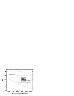
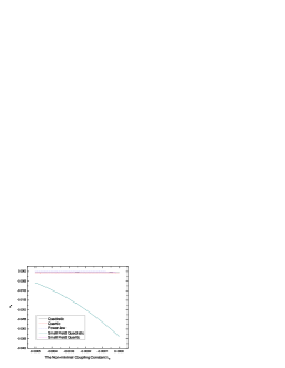
Figure 1: $n_{s}-1$ and $\alpha_{s}$ as functions of $\lambda_{0}$ in the models with $f=M_{p}^{2}R+\lambda_{0}\varphi^{2}R$. Red spectrum is common in this case except that the power-law potential gives a very small positive $n_{s}-1$. Running of spectral indices are quite small except in the small field quadratic inflation.

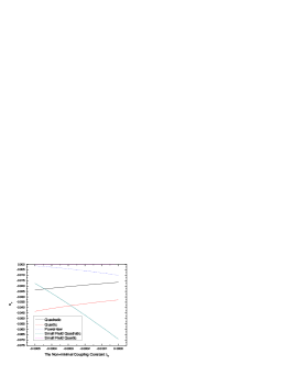
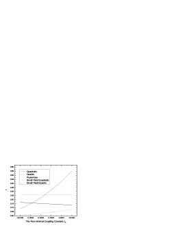
Figure 2: $n_{T}$ and $r$ as functions of $\lambda_{0}$ in the models with $f=M_{p}^{2}R+\lambda_{0}\varphi^{2}R$.

6.2 Models with $f=M_{p}^{2}R+\lambda_{0}M_{p}^{-2}\varphi^{2}R^{2}$

By COBE normalization condition and choosing the solution which smoothly reduces to the minimal case in the weak nonminimal coupling limit, $n_{s}-1$, $\alpha_{s}$, and $n_{T}$, $r$ are shown in Fig.3 and Fig.4 respectively. A red power spectrum is obtained in this case. A large running can be produced for some potentials when the nonminimal coupling is large. For the small field potential the large running is negative while the quadratic potential gives a positive large running.

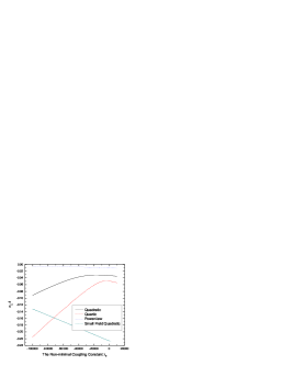
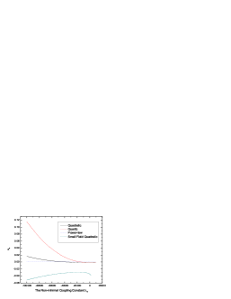
Figure 3: $n_{s}-1$ and $\alpha_{s}$ as functions of $\lambda_{0}$ in the models with $f=M_{p}^{2}R+\lambda_{0}M_{p}^{-2}\varphi^{2}R^{2}$ for the solution which has a smooth minimal coupling limit. The power spectrum is also red in all cases we consider. Large running can be produced when the absolute value of $\lambda_{0}$ is large, but only the small field quadratic potential produces a negative large running.

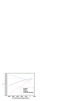
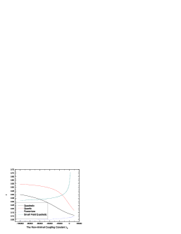
Figure 4: $n_{T}$ and $r$ as functions of $\lambda_{0}$ in the models with $f=M_{p}^{2}R+\lambda_{0}M_{p}^{-2}\varphi^{2}R^{2}$ for the solution which has a smooth minimal coupling limit. The small field quadratic potential model provide a positive $n_{T}$. Such phenomena never appears in the minimal models.

We note from these figures that the small field inflation with $V(\varphi)=\lambda(1-c\varphi^{2})$ is not favored by experiment when $\lambda_{0}\rightarrow 0$ because $n_{s}-1$ is too small and $r$ is too large. But when $\lambda_{0}$ is taken into consideration, this model behaves much better in both figures. We also observe that $n_{T}$ in the small field inflation can be positive, while in the minimal inflation model it is always negative. If in future experiments a blue spectrum of gravitational waves is detected, it may be a signal that nonminimal coupling effect should be considered.

Fig.5 presents $n_{s}-1$ and $\alpha_{s}$ as a function of $\ln(k/k_{c})$, where $k_{c}$ is where COBE normalization is taken, we assume it is 60 e-folds from the end of inflation. To know the exact e-folding number at COBE normalization point requires the knowledge of the details of reheating, which will not be considered in this paper.

Figure 5: $n_{s}-1$ and $\alpha_{s}$ as functions of $\ln(k/k_{c})$ in the models with $f=M_{p}^{2}R+\lambda_{0}M_{p}^{-2}\varphi^{2}R^{2}$ and the quadratic potential $V(\varphi)=\frac{1}{2}m^{2}\varphi^{2}$ for the solution which has a smooth minimal coupling limit. $\lambda_{0}$ is taken -50000 in both figures. $k_{c}$ is where the COBE normalization is taken. We assume at $k_{c}$, there are 60 e-folds of inflation. The power spectrum is red, with a positive running.

We find that something new happens here, if we take $\lambda_{0}\sim-60000$ and draw a figure like Fig.5. $F$ crosses zero at the largest scale that can be observed today, and the perturbations blow up during the zero-crossing. This region can not be treated exactly by the approach in this paper because the slow-roll conditions (9) and the expansion (22) break down. The exact equations of motion for the background shows that this region is indeed unusual. This phenomenon can also happen in some other models studied in this paper. This phenomenon may have something to do with the lower CMB anisotropy power on the largest angular scales. To make sure of this, a detailed calculation is required. Similar phenomenon in the quintessential models of dark energy is studied [16], but as far as we know, no consideration in inflation models and effects on the power spectrum is made.

The COBE normalization equation does not always have an unique solution. In some models, there can be additional solutions other than the solution studied above, namely, there are different regions where either $V$ or $f$ dominates. These new solutions can be much different from the minimal inflation models. In these models, a blue power spectrum is common and a negative running of the spectral index is possible. Large gravitational waves can be produced in these models, while in a large parameter region $r$ lies below the experimental upper bound. Models of this kind with the quadratic and quartic potential are drawn in Fig.6 and Fig.7.

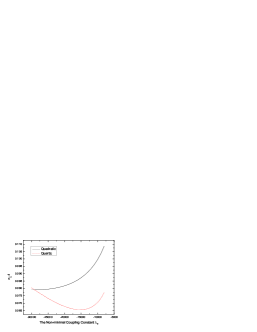
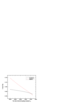
Figure 6: $n_{s}-1$ and $\alpha_{s}$ as functions of $\lambda_{0}$ in the models with $f=M_{p}^{2}R+\lambda_{0}M_{p}^{-2}\varphi^{2}R^{2}$ for the new solution in the nonminimal model. A blue power spectrum is produced in this case, with a negative running when the absolute value of $\lambda_{0}$ is not large.

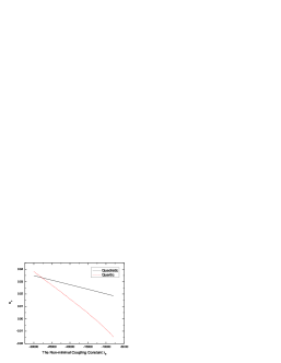
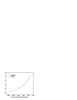
Figure 7: $n_{T}$ and $r$ as functions of $\lambda_{0}$ in the models with $f=M_{p}^{2}R+\lambda_{0}M_{p}^{-2}\varphi^{2}R^{2}$ for the new solution in the nonminimal model. Tensor mode perturbation is large in this solution, which may be approved or disapproved in the near future.

Fig.8 presents the $k$-dependence of $n_{s}-1$ and $\alpha_{s}$ for this solution. For the model we are considering, the running is not large enough for the blue spectrum to run to a red spectrum.

Figure 8: $n_{s}-1$ and $\alpha_{s}$ as functions of $\ln(k/k_{c})$ in the models with $f=M_{p}^{2}R+\lambda_{0}M_{p}^{-2}\varphi^{2}R^{2}$ and the quadratic potential $V(\varphi)=\frac{1}{2}m^{2}\varphi^{2}$ when $f$ dominates over $V$. $\lambda_{0}$ is taken -10000 in both figures. In order that $r$ is not too large, the running can not be large enough to change the blue spectrum to a red one.

By comparing with the $n_{3}=0$ minimal models and the corresponding figures for the models with $n_{3}=1$, we find that a large running is usually produced in $n_{3}=2$ models. While in the $n_{3}=1$ and $n_{3}=0$ case, it is difficult to produce such a large running except in the small field quadratic model.

It can be shown that the class of models $f=M_{p}^{2}R+\lambda_{0}M_{p}^{-4}\varphi^{4}R^{2}$ are quite similar to models $f=M_{p}^{2}R+\lambda_{0}M_{p}^{-2}\varphi^{2}R^{2}$, the only important difference is that in order to get the same $n_{s}-1$ and the running, $\lambda_{0}$ required in the former models are commonly 3 or 4 magnitudes smaller than that in the latter models.

6.3 Models with $f=M_{p}^{2}R+\lambda_{0}\exp(-\lambda_{1}\varphi/M_{p})R^{2}$

In this class of models, to make any differences from the minimal model, a very large $\lambda_{0}$ is required. A blue power spectrum can be produced with a large but positive running. $n_{s}-1$, $\alpha_{s}$, and $n_{T}$, $r$ are shown in Fig.9 and Fig.10 respectively.

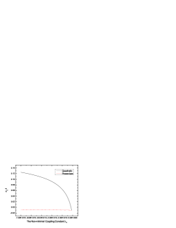
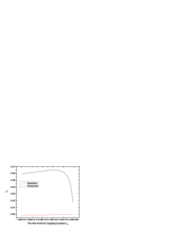
Figure 9: $n_{s}-1$ and $\alpha_{s}$ as functions of $\lambda_{0}$ in the the models with $f=M_{p}^{2}R+\lambda_{0}\exp(-\lambda_{1}\varphi)R^{2}$. A blue spectrum is produced in the quadratic potential, but the running is positive. A number $-1.00E+014$ in the figure denotes $-1.00\times 10^{14}$.

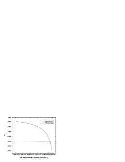
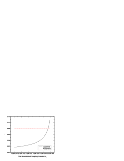
Figure 10: $n_{T}$ and $r$ as functions of $\lambda_{0}$ in the models with $f=M_{p}^{2}R+\lambda_{0}\exp(-\lambda_{1}\varphi)R^{2}$.

7 Conclusion

We obtained the scalar power spectrum $\mathcal{P}_{\mathcal{R}}$, the spectral index $n_{s}-1$, the running of the spectral index $\alpha_{s}$, the tensor mode spectral index $n_{T}$, and the ratio of the amplitude of tensor fluctuations to scalar fluctuations $r$ in this paper, they are given in equations (43), (44), (46), (48) and (49) respectively. We constructed a nearly-conserved quantity which can be used in models different from the single inflaton model with minimal coupling. It has a wide range of applicability. Also, a new consistency relation is given, which is subject to test in future experiments.

In the study of some concrete models, we see that there can be novel new features, such as a blue spectrum and a large running. We can also arrange $F$ properly in order to have a brief fast-rolling before the slow-rolling period. It has been shown that the problem of a large running of the spectral index is eased in our models in contrast to the minimal model or $f(\varphi)R$ coupling models.

The following issues deserve further investigation: The case when a nonminimal coupling becomes so strong that the quantum gravity effect destroys the usual canonical quantization picture at a length scale much smaller than the Hubble radius; the region where $F$ crosses zero, producing a sudden fast-roll stage during the period of slow-roll inflation. A more careful study of these issues may lead to very interesting physics.

Appendix A A General Nearly Conserved Quantity

From a general differential equation with two small parameters $\epsilon_{1}$ and $\epsilon_{2}$,

$$\ddot{\phi}+(1+\epsilon_{1})H\dot{\phi}+\epsilon_{2}H^{2}\phi+\frac{q^{2}}{a^{2}}\phi=0$$ (52)

The following quantity is nearly conserved when $q\ll aH$,

$$\mathcal{R}=c[\frac{1}{H}\dot{\phi}+(1+\epsilon_{1}+\frac{\dot{H}}{H^{2}}-\epsilon_{2})\phi]e^{\int\epsilon_{2}Hdt}$$ (53)

where c is a constant. $\dot{\mathcal{R}}/(H\mathcal{R})$ is of order $\mathcal{O}(\epsilon^{2})$ plus a term proportional to $q^{2}/a^{2}$.

$$\mathcal{\dot{R}}=c[\epsilon_{2}(\epsilon_{1}+\frac{\dot{H}}{H^{2}}-\epsilon_{2})H+\dot{\epsilon_{1}}+\left(\frac{\dot{H}}{H^{2}}\right)^{\cdot}-\dot{\epsilon_{2}}]\phi e^{\int\epsilon_{2}Hdt}-\frac{c}{H}\frac{q^{2}}{a^{2}}e^{\int\epsilon_{2}Hdt}$$ (54)

This construction is unique up to the constant $c$, and can be used in various cases where (52) is satisfied.

In the minimal inflation model, the equation (52) takes the form

$$\ddot{\phi}+(H-\frac{\ddot{H}}{\dot{H}})\dot{\phi}+(2\dot{H}-\frac{H\ddot{H}}{\dot{H}})\phi+\frac{k^{2}}{a^{2}}\phi=0$$ (55)

And $\mathcal{R}$ is the comoving curvature perturbation, which happens to be conserved to all orders in $\epsilon$.

In our nonminimal model, Inserting the Taylor expansion of ${\cal G}_{k}$ into (25), one can find

$$\phi{{}^{\prime\prime}}_{k}+(aH)\left(\frac{2\dot{G}_{0}}{H(1+G_{0})}+2\delta+3\gamma\right)\phi^{\prime}_{k}+q^{2}\phi_{k}$$

$$+(aH)^{2}\left(\frac{\dot{G_{0}}}{H(1+G_{0})}-\frac{4G_{0}}{1+G_{0}}\epsilon+\frac{3+G_{0}}{1+G_{0}}\gamma+2\delta\right)\phi_{k}=0,$$ (56)

where $q$ is a rescale of $k$ as in (29). So $\mathcal{R}$ can be written as

$$\mathcal{R}_{k}\equiv\frac{H}{\dot{H}}\dot{\phi}_{k}+\left(\frac{H^{2}}{\dot{H}}+2\frac{\dot{F}}{F}\frac{H}{\dot{H}}+\frac{\dot{G_{0}}}{1+G_{0}}\frac{H}{\dot{H}}-1\right)\phi_{k}$$ (57)

It is shown in Appendix B that calculations using the comoving curvature perturbation can also get correct results in our nonminimal model. But it can be shown that this fact is not generic in other generalizations of inflation models.

The only requirement for $\mathcal{R}$ to be nearly conserved is a diagonized equation of motion. So it can also be used in many other cases such as inflation models with holographic dark energy components [17] where entropy perturbation is produced and the comoving curvature perturbation is not a conserved quantity.

Appendix B Entropy-Perturbation-Like Sources

In the minimal inflation model, during inflation and the post-inflationary period before the comoving wave length re-enter the horizon, the pressure can be expressed as $p=p(\rho,S)$, where $\rho$ is the energy density and $S$ is the entropy density up to a normalization. If there is no entropy perturbation produced, just as in the single-field minimal inflation model, there is only one degree of freedom in the scalar type perturbations, so $p$ only depends on $\rho$. Then one can find

$$\frac{\dot{\rho}}{\dot{p}}=\frac{\delta\rho}{\delta p}$$ (58)

This relation has two consequences. First, when (58) is satisfied, the equations (19) and (20) can be diagonized into a one-variable differential equation exactly, as in the $f(R)$ or $f(\varphi)R$ gravity models, studied in [13]. Second, the comoving curvature perturbation is conserved in a model without entropy perturbation.

But in general, when entropy perturbation $\delta S$ is generated, the entropy perturbation can be defined as

$$\delta p=\frac{\dot{p}}{\dot{\rho}}\delta\rho+T\delta S$$ (59)

where $T$ is the temperature. It can be shown that

$$\dot{\tilde{\mathcal{R}}}=-\frac{H}{\dot{H}}\frac{T}{2M_{p}^{2}}\delta S+\mbox{terms proportional to}\frac{k^{2}}{a^{2}}$$ (60)

where $\tilde{\mathcal{R}}$ is the comoving curvature perturbation.

During inflation, $\tilde{\mathcal{R}}$ can be expressed as

$$\tilde{\mathcal{R}}=\psi-\frac{H}{\dot{H}}\left(\dot{\psi}+H\phi\right)$$ (61)

In nonminimal models, for general $f(\varphi,R)$, it is different from $\mathcal{R}$ introduced in Appendix A. From the uniqueness of $\mathcal{R}$, we conclude that $\delta S$ is nonzero. The existence of $\delta S$ can also be shown by direct calculations.

It is not surprising that the entropy perturbation is produced in our nonminimal models, because when we consider nonminimal models other than $f(R)$ or $f(\varphi)R$, one extra low energy effective degree of freedom opens up, and the entropy perturbation can be produced.

Although the entropy perturbation in our models exists and affects the evolution of scalar type perturbations, it can not live so long to have direct observable effects. To see this, we consider the period begin from a few e-folds outside the horizon, where the long wave length expansion can be applied to the Bessel function solution. During this period, $\psi$ and $\phi$ can be considered as slow-roll quantities, and the difference between time derivatives of $\mathcal{R}$ and $\mathcal{\tilde{R}}$ can be neglected. So

$$\frac{\dot{\tilde{\mathcal{R}}}}{H\tilde{\mathcal{R}}}=\mathcal{O}(\epsilon^{2}),$$ (62)

which means the entropy perturbation can be neglected a few e-folds after horizon crossing, and do not destroy the observational bounds. No extra decay mechanism for $\delta S$ is needed.

References

- [1] A. H. Guth, Phys. Rev. D 23, 347 (1981); A. D. Linde, Phys. Lett. B 108, 389 (1982); A.Albrecht and P. J. Steinhardt, Phys. Rev. Lett. 48, 1220 (1982)
- [2] Robert H. Brandenberger, “Challenges for String Gas Cosmology”, hep-th/0509099
- [3] D.N.Spergel et al., astro-ph/0603449
- [4] Q.-G. Huang and M, Li, astro-ph/0603782; X. Zhang and F.-Q, Wu, astro-ph/0604195, Phys. Lett. B638 (2006) 396; Q.-G. Huang, astro-ph/0605442; X. Zhang, hep-th/0608207; Q.-G. Huang, hep-th/0610389.
- [5] Q.G. Huang and M. Li, JHEP 0306(2003)014, hep-th/0304203; JCAP 0311(2003)001, astro-ph/0308458; Nucl.Phys.B 713(2005)219, astro-ph/0311378; S. Tsujikawa, R. Maartens and R. Brandenberger, astro-ph/0308169.
- [6] K. Izawa, hep-ph/0305286; S. Cremonini, hep-th/0305244; E. Keski-Vakkuri, M. Sloth, hep-th/0306070; M. Yamaguchi, J. Yokoyama, hep-ph/0307373; J. Martin, C. Ringeval, astro-ph/0310382; K. Ke, hep-th/0312013; S. Tsujikawa, A. Liddle, astro-ph/0312162; C. Chen, B. Feng, X. Wang, Z. Yang, astro-ph/0404419; L. Sriramkumar, T. Padmanabhan, gr-qc/0408034; N. Kogo, M. Sasaki, J. Yokoyama, astro-ph/0409052; G. Calcagni, A. Liddle, E. Ramirez, astro-ph/0506558; H. Kim, J. Yee, C. Rim, gr-qc/0506122.
- [7] A. Ashoorioon, J. Hovdebo, R. Mann, gr-qc/0504135; G. Ballesteros, J. Casas, J. Espinosa, hep-ph/0601134; J. Cline, L. Hoi, astro-ph/0603403.
- [8] B. Feng, M. Li, R. J. Zhang and X. Zhang, astro-ph/0302479; J. E. Lidsey and R. Tavakol, astro-ph/0304113; L. Pogosian, S. -H. Henry Tye, I. Wasserman and M. Wyman, Phys. Rev. D 68 (2003) 023506, hep-th/0304188; S. A. Pavluchenko, astro-ph/0309834; G. Dvali and S. Kachru, hep-ph/0310244.
- [9] M. Baldi, F. Finelli and S. Matarrese, astro-ph/0505552, Phys.Rev. D72 (2005) 083504; F. Finelli, M. Rianna and N. Mandolesi, astro-ph/0608277.
- [10] A. Starobinsky, “A new type of isotropic cosmological model without singularity”, Phys. Lett. B91 (1980) 99; “The perturbation spectrum evolving from a non-singular, initially de Sitter cosmology, and the microwave background anisotropy”, Sov. Astron. Lett. 9 (1983) 302.
- [11] V. Mukhanov and G. Chibisov, Pis’ma Zh. Eksp. Teor. Fiz. 33 (1981) 549.
- [12] L. Amendola, M. Litterio, and F. Occhionero, Int. J. Mod. Phys. A 5, 3861 (1990); A. Barroso, J. Casasayas, P. Crawford, P. Moniz, and A. Nunes, Phys. Lett. 275B, 264 (1992).
- [13] Jai-chan Hwang and Hyerim Noh, “Classical evolution and quantum generation in generalized gravity theories including string corrections and tachyon: Unified analyses”, Phys. Rev. D71, (2005) 063536, gr-qc/0412126
- [14] Miao Li, “Nonminimal Inflation and the Running Spectral Index”, astro-ph/0607525, JCAP10 (2006) 003.
- [15] Viatcheslav F. Mukhanov, H. A. Feldman and Robert H. Brandenberger, “Theory of cosmological perturbations”, Phys. Rept. 215,(1992) 203
- [16] Edgard Gunzig, Alberto Saa, “Conformal quantum effects and the anisotropic singularities of scalar-tensor theories of gravity ”, Int.J.Theor.Phys. 43 (2004) 575-583, gr-qc/0406069.
- [17] M. Li, “A Model of Holographic Dark Energy ”, Phys.Lett. B603 (2004) 1, hep-th/0403127; Q.-G. Huang and M, Li, “The Holographic Dark Energy in a Non-flat Universe”, JCAP 0408 (2004) 013, astro-ph/0404229. B. Chen, M. Li and Y. Wang, work in progress.