X-Ray Emission from Planetary Nebulae Calculated by 1D Spherical Numerical Simulations

Abstract

We calculate the X-ray emission from both constant and time evolving shocked fast winds blown by the central stars of planetary nebulae (PNs) and compare with observations. Using spherically symmetric numerical simulations with radiative cooling, we calculate the flow structure, and the X-ray temperature and luminosity of the hot bubble formed by the shocked fast wind. We find that a constant fast wind gives results that are very close to those obtained from the self-similar solution. We show that in order for a fast shocked wind to explain the observed X-ray properties of PNs, rapid evolution of the wind is essential. More specifically, the mass loss rate of the fast wind should be high early on when the speed is $\sim 300-700~{}\rm{km}~{}\rm{s}^{-1}$, and then it needs to drop drastically by the time the PN age reaches $\sim 1000~{}\rm{yr}$. This implies that the central star has a very short pre-PN (post-AGB) phase.

Subject headings: Subject headings: stars: mass loss stars: winds, outflows planetary nebulae: X-ray X-rays: ISM

1 INTRODUCTION

In the last seven years people have been trying to understand the nature and the origin of the extended, spatially resolved X-ray emission detected in planetary nebulae (PNs) by the Chandra X-ray Observatory (CXO), e.g., BD +30^∘3639 (Kastner et al. 2000; Arnaud et al. 1996 detected X-rays in this PN with ASCA), NGC 7027, (Kastner, et al. 2001), NGC 6543 (Chu et al. 2001), Henize 3-1475 (Sahai et al. 2003), Menzel 3 (Kastner et al. 2003), and by the XMM-Newton X-ray Telescope, e.g., NGC 7009 (Guerrero et al. 2002), NGC 2392 (Guerrero et al. 2005), and MGC 7026 (Gruendl et al. 2004). The X-ray emitting gas can come from shocked fast wind segments that were expelled by the central star during the late post-asymptotic giant branch (AGB) phase and/or early PN phase, and/or the X-ray emitting gas may result from a collimated fast wind (CFW), or jets, blown in conjunction with the companion to the central star during the late AGB phase or early post-AGB phase (Soker & Kastner 2003). These interactions play a significant role in shaping PNs (e.g., Balick & Frank 2002, and references therein). Therefore, understanding the X-ray emission can teach us about the properties of the central fast wind and CFW, and by that shed light on the shaping mechanism of PNs.

One of the major properties of the X-ray emitting gas to be understood is its relatively low temperature of $\sim 1-3\times 10^{6}~{}\rm{K}$. The observed velocity of fast winds in PNs is $v_{f}>1000~{}\rm{km}~{}\rm{s}^{-1}$, implying a post shock temperature of $T>10^{7}~{}\rm{K}$, much higher than observed in the X-ray emitting gas. Two solutions are possible: (1) The hot ($T>10^{7}~{}\rm{K}$) post-shock gas is cooled via heat conduction by interaction with the cold, slow-wind material, which is at a temperature of $T\sim 10^{4}~{}\rm{K}$ and most X-ray emission comes from the conduction front (Soker 1994; Zhekov & Perinotto 1996; Steffen et al. 2005). A similar effect can result from mixing of hot post-shock fast-wind gas and cool slow-wind gas (Chu et al. 1997). Instability modes near the contact discontinuity can lead to significant mixing of cold and hot gas (Stute & Sahai 2006, hereafter SS06). (2) The X-ray emitting gas comes mainly from a slower moderate-velocity wind of $v_{f}\sim 500~{}\rm{km}~{}\rm{s}^{-1}$. This flow can be a post-AGB wind from the central star (Soker & Kastner 2003; Akashi et al. 2006 hereafter ASB06; and SS06), or two opposite jets (or CFW, Soker & Kastner 2003). The idea of a post-AGB wind is supported by the analytical calculations of a spherically- symmetric fast wind done by ASB06 and based on the self-similar solution of Chevalier & Imamura (1983). The self similar solutions, however, are limited in their ability to account for temporal evolution and to properly treat radiative cooling.

In the present paper, we carry out a numerical study for the expected contribution from the fast spherical wind blown by the central star. We run numerical simulations solving the hydrodynamical equations with a full treatment of radiative cooling, and by setting proper initial and boundary conditions of the interacting winds, e.g., a fast wind evolving with time. Some of the results obtained here are similar to results obtained very recently by SS06. The remainder of the paper is outlined as follows: The numerical method is described in §2. In §3 we compare the spherical symmetrical numerical simulations with the self-similar results of ASB06. In §4 we present several cases of a time evolving fast wind. A short summary is given in §5.

2 NUMERICAL METHOD

The simulations were performed using Virginia Hydrodynamics-I (VH-1), a high resolution multidimensional astrophysical hydrodynamics code developed by John Blondin and co-workers (Blondin et al. 1990 ; Stevens et al. 1992; Blondin 1994). The code uses finite-difference techniques to solve the equations of an ideal inviscid compressible fluid flow. We use 1024 grid points to resolve the calculated region. The distance between adjacent grid points increase as the flow expands. Using more or less grid points (e.g., 512) changes the results only by a few per cents or less. Radiative cooling was incorporated for gas temperatures above $10^{4}~{}\rm{K}$, using the cooling function $\Lambda(T)$ for solar abundances from Sutherland & Dopita (1993; their table 6). Radiative cooling should be treated carefully near the contact discontinuity. The hot bubble cools slowly because of its low density, while the dense shell cools slowly because of its low temperature ($T=10^{4}~{}\rm{K}$) where the cooling rate is low. The one or two grid points at the interface between the hot bubble and cold shell could share high temperature from the bubble and high density from the cold shell. Therefore, radiative cooling at the interface may be overestimated. Actually, low resolution in the code might in a sense mimic heat conduction. Our code includes a check of this numerical problem. It takes for the cooling rate at the contact discontinuity the minimum cooling rate of the two zones (either from the cold shell or from the bubble).

To mimic the ionizing radiation of the central star, we did not let the gas to cool to temperatures below $10^{4}~{}\rm{K}$ when radiative cooling was included. For the initial conditions we take a spherically symmetric slow wind with a constant mass loss rate $\dot{M}_{1}$ and a constant velocity $v_{1}=10~{}\rm{km}~{}\rm{s}^{-1}$. The slow wind fills the space around the center from a minimum initial radius $R_{c0}=R_{c}(t=0)$. This implies that the initial density is $\rho_{1}=\dot{M}_{1}/4\pi v_{1}r^{2}$ for $r>R_{c0}$ and zero inside this radius. At time $t=0$ a spherically symmetric fast wind with a mass loss rate of $\dot{M}_{2}(t)$ and a velocity $v_{2}(t)$ is turned on close to the center.

The reasons for setting up a vacuum in the center of the slow wind before the fast wind is turned on are: (1) There is a large uncertainty as to the evolution of the wind in the transition from the AGB phase to the PN phase. Therefore, there is no clear parameters to use for the wind at this stage. (2) This wind period has relatively low mass, as mass loss rate is lower than in the AGB phase. On the other hand, it is dense and slow enough to cool very rapidly. So practically, it will form a shell inward to the slow wind. As far as the numerical procedure is concerned, we can mimic this intermediate wind segment by changing the value of $R_{c0}$. As we show here, this does not change our results much.

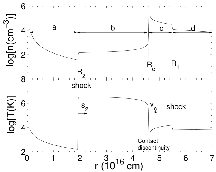
Figure 1: Total number density (upper panel) and temperature (lower panel) at $t=400~{}\rm{yr}$ from a spherical symmetric constant-flow simulation with no radiative cooling included, and with the following parameters: Mass loss rate and velocity of the slow wind: $\dot{M}_{1}(t)=7\times 10^{-6}M_{\odot}~{}\rm{yr}^{-1}$ and $v_{1}(t)=10~{}\rm{km}~{}\rm{s}^{-1}$. Mass loss rate and velocity of the fast wind: $\dot{M}_{2}(t)=1.4\times 10^{-7}M_{\odot}~{}\rm{yr}^{-1}$ and $v_{2}(t)=500~{}\rm{km}~{}\rm{s}^{-1}$. The marked regions are: ($a$) undisturbed central star fast wind; (b) Hot bubble; (c) Shocked slow wind; and (d) Unshocked nebular gas (AGB wind). $v_{c}$ and $s_{2}$ represent the velocities of the contact discontinuity and inner shock, respectively.

The results of one run with a non-evolving fast wind of $\dot{M}_{2}(t)=1.4\times 10^{-7}M_{\odot}~{}\rm{yr}^{-1}$ and $v_{2}(t)=500~{}\rm{km}~{}\rm{s}^{-1}$, but without radiative cooling, is shown in Fig. 1 at time $t=400~{}\rm{yr}$. $R_{c0}=3\times 10^{15}~{}\rm{cm}$ in this run. In all runs $t=0$ is when the fast wind starts. In this run, $\dot{M}_{1}=7\times 10^{-6}M_{\odot}~{}\rm{yr}^{-1}$ (more examples can be found in SS06.) The fast wind collides with the slow wind and two spherical shock waves are formed. One shock moves outwards at radius $R_{1}(t)$ into the undisturbed slow wind, while an inner shock runs into the expanding undisturbed fast wind at radius $R_{2}(t)$. Between the two shock fronts lies the contact discontinuity at radius $R_{c}(t)$ (see also Fig. 2 by Volk & Kwok 1985). The values of the density and the temperature jump across the contact discontinuity, while the velocity and pressure vary continuously across it. The volume inside the dense shell $R_{2}<r<R_{c}$ (region $b$) in runs without radiative cooling is filled with hot shocked fast wind. When radiative cooling is included, the relatively dense region behind the contact discontinuity cools radiatively and forms a cold layer at $T\sim 10^{4}~{}\rm{K}$ of previously shocked fast wind material. The volume filled with hot X-ray emitting gas is termed the hot bubble (region b). The shocked slow wind in the shell $R_{c}<r<R_{1}$ (region $c$) cools much faster due to its high density maintaining a temperature of $\sim 10^{4}~{}\rm{K}$.

We are interested in the X-ray luminosity $L_{x}$ and temperature of the hot gas. The luminosity is calculated in the energy band $0.2-10~{}\rm{keV}$, as described in ASB06. This range is chosen to reflect approximately the sensitivity regime of the Chandra and XMM-Newton telescopes and science instruments. As discussed by SS06, for gas temperatures of $T_{x}\lesssim 3\times 10^{6}~{}\rm{K}$ most of the cooling takes place via emission at lower energies ($<0.2$ keV), which is outside the range of the instruments we compare our results with. The temperature of the X-ray emitting gas in the hot bubble varies with radius (see Fig. 1). In ASB06 (eq. 9 therein), we introduced a mean emission-measure weighted temperature $T_{x}$ that would be deduced from a single-temperature model for the X-ray spectrum. Here too, we will refer to the mean temperature of the hot bubble as $T_{x}$.

In the numerical model, the flow relaxes to a more or less steady state after $\sim 100$ yr. For several hundred years, the velocity of the contact discontinuity, $v_{c}$, and the velocity of the inner shock, $s_{2}$, oscillate around their mean values. However, the influence of these oscillations on the observed X-ray luminosity and temperature is very small. At the first encounter of the fast wind with the slow wind, the temperature of the X-ray emitting gas is that of the post-shock gas. After $\sim 100$ yr, as the post-shock gas expands with the nebula, the hot bubble cools, and $T_{x}$ decreases as most of the radiation comes from the region close to the contact discontinuity. Some other flow properties at the very early stages of the winds interaction process, are discussed by SS06. SS06 compare also the velocity of the contact discontinuity in their numerical simulations with analytical expressions. For the run presented in Fig. 1, we find $v_{c}=36.2~{}\rm{km}~{}\rm{s}^{-1}$. This run is referred to as model B5 in ASB06 and in SS06, with the difference that ASB06 and SS06 took the undisturbed slow wind temperature to be very low, $T\ll 10^{4}~{}\rm{K}$, while here $T=10^{4}~{}\rm{K}$. The self-similar solution with a cold slow wind ($T\ll 10^{4}~{}\rm{K}$) gives $v_{c}=32.6~{}\rm{km}~{}\rm{s}^{-1}$. The higher temperature here ($T=10^{4}~{}\rm{K}$) implies more energy in the flow, hence larger $v_{c}$. When SS06 take $T\ll 10^{4}~{}\rm{K}$ and include radiative cooling, they find $v_{c}=27~{}\rm{km}~{}\rm{s}^{-1}$, as a consequence of the loss of energy by radiation. The actual temperature of the undisturbed slow wind will rise from a few $100~{}\rm{K}$ during the pre-PN (PPN) phase to $\sim 10^{4}~{}\rm{K}$ during the PN phase, after ionization starts. Neither we nor SS06 treat this full evolution as we do not include photo-heating. We prefer to take the temperature as appropriate for the PN phase, while SS06 take the PPN-phase temperature. This is not a major issue, as the temperature of the pre-shock slow wind affects only slightly the X-ray properties. On another matter, residual differences between our results and those of SS06 can be attributed to slight numerical differences in fitting the cooling function given by Sutherland & Dopita (1993).

At early times, the X-ray emission of the PN depends strongly on the slow wind initial radius $R_{c0}$. This is demonstrated in Fig. 2, which shows the PN evolution with time in the $L_{x}-T_{x}$ plane for three different initial inner radii $R_{c0}$. As explained above, the temperature is high at very early times, and decreases toward its self similar solution at later times. At early times the X-ray luminosity is very low as there is not much gas in the hot bubble. With time, the X-ray luminosity increases as more mass is accumulated in the hot bubble (SS06) until the effect of expansion takes over, the temperature stabilizes and the X-ray luminosity decreases as in the self similar solution (see next section). To reach the self similar behavior takes more time for larger values of $R_{c0}$, but regardless of $R_{c0}$ all simulations converge to the same results as seen in Fig. 2. Therefore, we will not discuss the very early times of evolution. In most runs, those lasting 5000 yr, we took $R_{c0}=8\times 10^{15}~{}\rm{cm}$. In the shorter runs, lasting 2000 yr, we took $R_{c0}=3\times 10^{15}~{}\rm{cm}$.

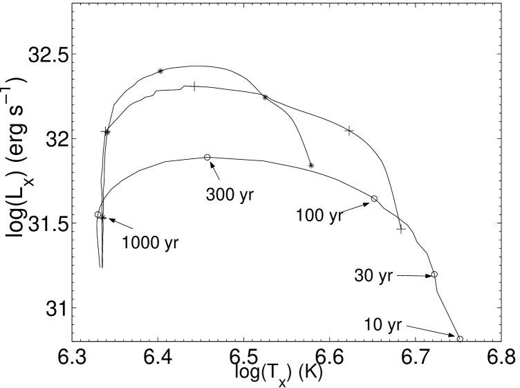
Figure 2: Simulated evolution of PN X-ray emission from $t=10$ yr to $t=1000$ yr for three cases differing by their initial inner radii of the slow wind: $R_{c0}=3\times 10^{15}~{}\rm{cm}$ (asterisks); $R_{c0}=5\times 10^{15}~{}\rm{cm}$ (plus signs); $R_{c0}=1.2\times 10^{16}~{}\rm{cm}$ (circles). Data points for all runs are given at five times as marked on the lower plot. In all runs $v_{1}(t)=10~{}\rm{km}~{}\rm{s}^{-1}$ (as in the rest of the paper), $\dot{M}_{1}(t)=7\times 10^{-6}M_{\odot}~{}\rm{yr}^{-1}$, $\dot{M}_{2}(t)=1.4\times 10^{-7}M_{\odot}~{}\rm{yr}^{-1}$, and $v_{2}(t)=500~{}\rm{km}~{}\rm{s}^{-1}$.

In order to demonstrate the effect of radiative cooling, we present in Fig. 3 a comparison between simulations with and without radiative cooling. The effect of radiative cooling is most pronounced at the densest and coolest shocked fast wind segments, which reside right behind the contact discontinuity. As explained above, no gas has a temperature below $10^{4}~{}\rm{K}$. In the hot bubble, generally $10^{5}<T<10^{7}~{}\rm{K}$ and the radiative cooling time $\tau_{\rm cool}$ is highly sensitive to the temperature ($\sim T^{5/2}$). This explains the sharp boundary of the radiatively cooled region marked as $RC$ in Fig. 3. We note that the region marked $RC$ is found to be the point where the radiative cooling time equals six times the age of the flow. Namely, regions with cooling time much longer that the flow time had time to cool. The reason why these regions had time to cool is that the gas now residing near the contact discontinuity (at $R_{c}$) was shocked at much smaller radius, and hence its density was higher and radiative cooling time much shorter in the past. Therefore, we would expect that the present radiative cooling time at $R_{c}$ is longer than the flow age.

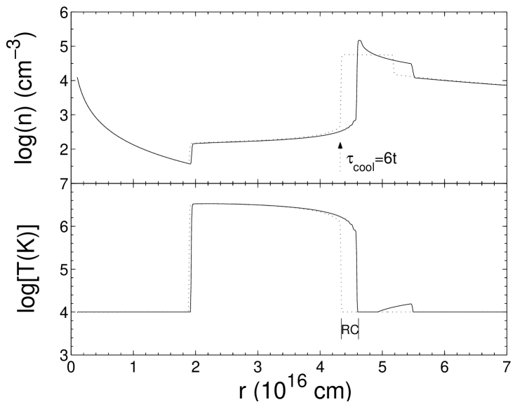
Figure 3: Simulation results for density and temperature profiles with and without cooling. The solid lines are the same as in Fig. 1, except that $T=10^{4}~{}\rm{K}$ was set as a strict lower limit. The dashed lines show the results for the same parameters, but with radiative cooling included. The region marked $RC$ is the region where radiative cooling is most effective. It is found to be the point where the radiative cooling time equals six times the age of the flow. It is seen that radiative cooling reduces the pressure in the hot bubble and hinders its expansion.

3 CONSTANT FAST WIND

We run several simulations with a constant, unevolving fast wind, namely, $\dot{M}_{2}(t)$ and $v_{2}(t)$ do not vary with time. The results enable a comparison with the self-similar results of ASB06 and serve as reference for the evolving fast wind simulations to be discussed in the next section. Radiative cooling is included in all runs in this section. We recall that in order to account for radiative cooling in the self similar solutions, we simply disregard wind segments with cooling times shorter than the PN age ($t_{\rm cool}<t$, see ASB06) in calculating the X-ray emission.

A comparison of the simulation results with the self-similar solutions is presented in Fig. 4 in terms of the PN evolution in the $L_{x}-T_{x}$ plane. Three cases are shown. The fast wind mass loss rate $\dot{M}_{2}$ in units of $10^{-7}M_{\odot}~{}\rm{yr}^{-1}$ is marked next to each track inside square brackets [ ], while the fast wind speed in units of $~{}\rm{km}~{}\rm{s}^{-1}$ is in parentheses ( ). The mass loss rate of the slow wind is $\dot{M}_{1}=7\times 10^{-6}M_{\odot}~{}\rm{yr}^{-1}$ and the slow wind speed is $v_{1}=10~{}\rm{km}~{}\rm{s}^{-1}$ in all runs. Short straight lines connect the self similar results to the numerical results at the same age $t$. Evidently, the self similar solutions with our approximation for radiative cooling provide very good estimates to the X-ray properties of the nebula. In all cases presented in Fig. 4, the self similar solutions reproduce $T_{x}$ and $L_{x}$ to within $\sim 30\%$ and $\sim 45\%$, respectively, of the simulation values. For ages of 200 yr and more, the self similar results for $T_{x}$ and $L_{x}$ are good to within $\sim 12\%$ and $\sim 30\%$. Recall that the simulation results at early times are uncertain as discussed in §2. It can be seen in the figure, that using less strict criteria for omitting fast-cooling wind segments (e.g., $t_{\rm cool}<3t$) improves the late-time self similar results at the price of larger discrepancies at earlier times. For the higher velocity simulations (two right cases in Fig. 4) the radiative cooling removes cooler gas more efficiently at early times, hence the temperature is higher than at later times. For the slower fast wind case, $v_{2}=400~{}\rm{km}~{}\rm{s}^{-1}$, the post shock temperature is low and density high, such that radiative cooling is very efficient. Because of that the entire shocked fast wind is cooling at early times. This explains its low temperature at early times.

In all cases, the general behavior of $L_{x}\propto t^{-\eta}$ with $\eta\sim 0.9$ is obtained. This dependence on time can be understood as follows. The velocity of the contact discontinuity $v_{c}$, is constant, hence the volume $V$, of the hot bubble increases as $V=4\pi(R_{c}^{3}-R_{2}^{3})/3\sim 4\pi(v_{c}t)^{3}/3$, and the density decreases as $n\propto(\dot{M}_{2}t)/V\propto t^{-2}$. As the temperature does not change much, the emissivity (power per unit volume) $\epsilon$ goes as $\epsilon\propto n^{2}\Lambda(T)\propto n^{2}\propto t^{-4}$, and $L_{x}=V\epsilon\propto t^{-1}$. This simple explanation, and the close fit of the numerical results to the self-similar solution with cooling gas removed (Fig. 4), enhance our confidence in our results. We find $R_{c}\propto t^{0.98}$ and the density inside the bubble to vary as $\rho\propto t^{-2}$, which gives for the mass in the bubble $M\propto~{}t^{0.94}$. As more mass cools with time, we expect less mass to be in the bubble. SS06 find in their numerical simulations $\eta=0.37$. We have no explanation for this discrepancy, but we note that SS06 find the mass in their X-ray bubble to increase as $~{}t^{1.5}$, rather than the simple expectation of $\sim t$. They explain it by more efficient cooling at early times. However, we note that this behavior continues to late times, $t>2000~{}\rm{yr}$ where the contact discontinuity is already at $r\simeq 10^{17}~{}\rm{cm}$.

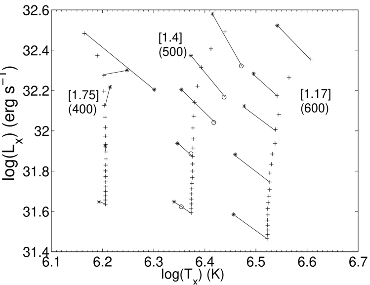
Figure 4: Comparison of PN evolution tracks in the $L_{x}-T_{x}$ plane between the full simulations (+ signs, top to bottom from 40 yrs to 800 yrs, every 40 yrs) and the self similar solutions (* signs at 40, 120, 200, 400, and 800 yrs). Radiative cooling was included in the self similar calculations by disregarding wind segments with $\tau_{\rm cool}<t$ for the X-ray emission. Equal-time data points are connected by lines to facilitate the comparison. The three cases considered differ by their $[\dot{M}_{2}/10^{-7}M_{\odot}~{}\rm{yr}^{-1}]$ and $(v_{2}/~{}\rm{km}~{}\rm{s}^{-1})$ values as indicated. $\dot{M}_{1}=7\times 10^{-6}M_{\odot}~{}\rm{yr}^{-1}$ and the initial slow wind temperature is $10~{}\rm{K}$ in all runs. Circles ($\circ$) in the middle run mark the self similar results in which wind segments with $\tau_{\rm cool}<3t$ were disregarded.

The results of the numerical simulations with constant fast wind properties strengthen our conclusions from self similar calculations (ASB06; see also SS06). Basically, X-ray emission from PNs can be accounted for by shocked wind segments that were expelled during the early PN phase, if the fast wind speed is moderate, $v_{2}\sim 400-600~{}\rm{km}~{}\rm{s}^{-1}$, and the mass loss rate is a few$\times 10^{-7}M_{\odot}~{}\rm{yr}^{-1}$. More generally, the X-ray emission from PNs can be accounted for by material ejected at speeds of $v_{2}\sim 400-600~{}\rm{km}~{}\rm{s}^{-1}$, whether from the central star during the post-AGB or from a companion blowing jets at the very late AGB phase (Soker & Kastner 2003). This fast flowing gas hits the slow wind, and passes through a shock wave. The post-shock gas is the X-ray emitter. In the next section we study more realistic, evolving fast winds in an attempt to further constrain the fast wind properties, which can produce observed X-ray emission of PNs. The bipolar X-ray morphology of several observed PNs, which indicates an important role of jets rather than a spherical fast wind, cannot be explained by the flows studied in this paper, and will be studied with a 2D numerical code in a future paper.

A comment on the mass loss rate and the alternative heat conduction model is needed here. Observations of mass loss rates during the PN phase show very low mass loss rates, $\dot{M}_{2}\lesssim 10^{-8}M_{\odot}~{}\rm{yr}^{-1}$, and high speeds, $v_{2}\gtrsim 1000~{}\rm{km}~{}\rm{s}^{-1}$, (Cerruti-Sola & Perinotto 1989; Perinotto et al. 1989). As shown by ASB06, such winds cannot account for the X-ray emission as the luminosity will be too low and temperature too high. This led to the idea of a heat conduction front between the hot bubble and the cold slow wind gas (Soker 1994). The density and temperature in the heat conduction front are intermediate, between those of the hot bubble and the cool slow wind gas. Heat conduction can make a significant effect and is required to explain the X-ray emission only if after the AGB wind there is a sharp transition to the PN-phase wind. Indeed, Zhekov & Perinotto (1996) in calculating the effect of heat conduction used a fast wind mass loss rate of $\dot{M}_{2}=7\times 10^{-9}M_{\odot}~{}\rm{yr}^{-1}$ for a fast wind speed of $v_{2}\simeq 500~{}\rm{km}~{}\rm{s}^{-1}$. Namely, the heat conduction model is based on the assumption that the relatively high mass loss rate ceases before the post-AGB wind speed reaches $v_{2}\sim 400~{}\rm{km}~{}\rm{s}^{-1}$. This type of wind implies a relatively long post-AGB evolution.

A different scenario would be a dense post-AGB wind, i.e., one in which the mass loss rate stays relatively high until later times, at least until the fast wind speed increases to $v_{2}\sim 600~{}\rm{km}~{}\rm{s}^{-1}$ (Soker & Kastner 2003; ASB06). These are the type of winds considered here in Fig. 4. Heat conduction, even if it exists here, will not change much, as the density of the hot bubble is already high enough for radiative cooling to be important, as seen in Fig. 3. This can be demonstrated as follows. At early times the pressure in the hot bubble is larger and temperature lower that that assumed in the heat conduction model (Soker 2004). Substituting a pressure of $nT=3\times 10^{8}~{}\rm{cm}^{-3}~{}\rm{K}$ and a temperature of $T_{h}=2.5\times 10^{6}~{}\rm{K}$, as appropriate near the contact discontinuity (see Fig. 3), in equation (6) of Soker (1994), we find that radiative losses become important already at an age of $t\simeq 500~{}\rm{yr}$. In the case of a very hot bubble ($T_{h}=10^{7}~{}\rm{K}$), as assumed by Soker (1994), radiative losses dominate at much later times, $t>10,000~{}\rm{yr}$.

There are several reasons to prefer the dense post-AGB wind scenario: (1) Even weak magnetic fields, which are likely to exist to some level in all post-AGB stars, will inhibit almost completely heat conduction. It is still possible that mixing occurs there (Chu et al. 1997), e.g., via turbulence (see the 2D simulations of SS06). (2) A large fraction of the X-ray bright PNs are very young (Soker & Kastner 2003), showing that the transition from the AGB to the PN phase is short. This implies a high mass loss rate during the post-AGB phase. (3) The strong X-ray emitting PN BD +30^∘3639 (PN G064.7+05.0) currently has a wind speed of $\sim 700~{}\rm{km}~{}\rm{s}^{-1}$ (Leuenhagen et al. 1996) as assumed in the dense fast wind model, and much slower than required in the heat conduction model. However, we caution that it is possible that the X-ray emission in this PN results from a CFW (jets), and not from the central fast wind. To summarize, at this stage both mechanisms in which the X-ray emitting gas is blown by the central star should be examined, as we cannot rule out that in some PNs the X-ray emission source is a heat conduction front (Soker 1994; Zhekov & Perinotto 1996; Steffen et al. 2005). However, at this point we favor the denser post-AGB model, which is the subject of this paper.

4 TIME VARYING FAST WIND

4.1 General Considerations

The conclusion of the previous section, which strengthens previous results (Soker & Kastner 2003, ASB06, and SS06) is that the fast wind segments that account for the X-ray emission should have speeds of $v_{2}\simeq 400-600~{}\rm{km}~{}\rm{s}^{-1}$, and the mass loss rate should be $\dot{M}_{2}\sim 10^{-7}M_{\odot}~{}\rm{yr}^{-1}$. Thus, within a few hundred years the mass of the relevant X-ray emitting plasma would be a few times $\sim 10^{-5}M_{\odot}$. The fast wind, however, evolves with time. In this section we assume that the X-ray emitting gas in PNs comes from a spherically symmetric central stellar wind, and use the X-ray properties of PNs to learn about and constrain the evolution of the fast wind. The fast wind evolution depends on the mass of the central star (e.g., Villaver et al. 2002), and possibly on an interaction with a companion. There are many uncertainties, and several different functions for the dependence of the fast wind mass loss rate and velocity on time have been proposed (e.g., Mellema 1994; Villaver et al. 2002; Perinotto et al. 2004; Garcia-Segura et al. 2006). To demonstrate the basic properties of an evolving fast wind, we consider several types of fast wind evolution.

Since slow winds can not produce X-rays, we start our simulations from when the fast wind speed is already $v_{2}\simeq 200-300~{}\rm{km}~{}\rm{s}^{-1}$, which is after the PN stage has already started (for example, we assume minimum temperature of $10^{4}~{}\rm{K}$ due to ionization by the central star). When comparing to observations, the real dynamical age of the PN, thus, is larger than the time (age) of the simulations by several hundred years. Our goal is to conduct a general study to find the influence of the different parameters on the X-ray emission, rather than to fit each PN with an appropriate mass loss evolution.

4.2 Different Simulated Cases

The strategy of varying the wind speed is to take an initial velocity of $v_{20}=300~{}\rm{km}~{}\rm{s}^{-1}$ and to allow it to increase gradually to currently observed speeds. The rise in velocity is assumed to take place over a typical time $\tau_{v}=1000$ yr. For simplicity, we start by assuming that the rise in velocity is linear.

$$v_{2}=v_{20}\left(1+\frac{t}{\tau_{v}}\right).$$ (1)

Our different cases are summarized in Table 1.

Table 1: Cases Calculated in section 4.2

Run	$\dot{M}_{1}$	$\dot{M}_{2}$	$v_{1}$	$v_{2}$	$\tau_{v}$
	$M_{\odot}~{}\rm{yr}^{-1}$	$M_{\odot}~{}\rm{yr}^{-1}$	$~{}\rm{km}~{}\rm{s}^{-1}$	$~{}\rm{km}~{}\rm{s}^{-1}$	yr
A	$10^{-5}$	$3\times 10^{-7}(v_{20}/v_{2})$	$10$	$eq.1$	1000
B.1	$10^{-5}$	$3\times 10^{-7}(v_{20}/v_{2})^{2}$	$10$	$eq.1$	1000
B.2	$10^{-4}$	$3\times 10^{-7}(v_{20}/v_{2})^{2}$	$10$	$eq.1$	1000
B.3	$10^{-4}$	$3\times 10^{-7}(v_{20}/v_{2})^{2}$	$10$	$eq.1$	500
B.4	$10^{-4}$	$10^{-6}(v_{20}/v_{2})^{2}$	$10$	$eq.1$	1000
C	$10^{-4}$	From P04	10	From P04	_

Notes: (1) $\tau_{v}$ is defined in equation (1). (2) P04 refers to Perinotto et al. (2004).

We first consider two versions of wind evolution.

(A) Constant momentum deposition rate $\dot{p}_{2}=\dot{M}_{2}v_{2}$, i.e. decreasing $\dot{M}_{2}=3\times 10^{-7}(v_{20}/v_{2})M_{\odot}~{}\rm{yr}^{-1}$. The evolution of the X-ray emission in the $L_{x}-T_{x}$ plane for this case with $\dot{M}_{1}=10^{-5}M_{\odot}~{}\rm{yr}^{-1}$ (as in all cases here $v_{1}=10~{}\rm{km}~{}\rm{s}^{-1}$) is shown in Fig. 5 by the ${}^{\prime}+^{\prime}$ symbols. The results are shown from $t=250~{}\rm{yr}$ to $t=5000~{}\rm{yr}$, with marks given every thousand years. It can be seen that $T_{x}$ increases with the velocity, while $L_{x}$ decreases since $\dot{M}_{2}$ decreases. The total mass that is lost to the fast wind over $2000~{}\rm{yr}$ is $\Delta M_{w2}=3.3\times 10^{-4}M_{\odot}$. This is approximately the mass available for the wind. Therefore, one could expect the wind in this model to cease after $\sim 2000~{}\rm{yr}$.

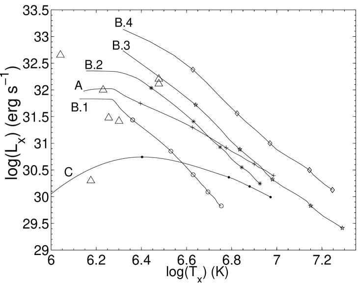
Figure 5: Evolution of X-ray emission from $t=250$ yr to $t=5000$ yr for the evolving-wind cases described in §4.2. Symbols are plotted every 1000 years. Plus signs show the constant momentum deposition case (A). Constant luminosity cases B.1 – B.4 are represented respectively by circles, asterisks, stars, and diamonds. Dots show the evolution for the wind according to Perinotto et al. (2004) for which the $t=1000$ yr mark is beyond the scale of the graph to the left. Triangles represent observed PNs which are listed in Table 2. All simulations at late times predict bright, detectable, high-$T_{X}$ PNs that are not observed implying that the wind must evolve (i.e. $\dot{M}_{2}(t)$ must decrease) faster than in these models.

(B) Constant kinetic power (luminosity) $\dot{E}_{2}=(1/2)\dot{M}_{2}v_{2}^{2}$, which together with equation (1) implies a decreasing mass loss rate: $\dot{M}_{2}=\dot{M}_{20}(v_{20}/v_{2})^{2}$. The total mass lost in the fast wind in this case is $\Delta M_{w2}=\dot{M}_{20}\tau_{v}$. We consider several cases with constant kinetic power.

(B.1) First, we take the typical parameter values: $\dot{M}_{2}=3\times 10^{-7}(v_{20}/v{2})^{2}M_{\odot}~{}\rm{yr}^{-1}$, $\tau_{v}=1000~{}\rm{yr}$, $v_{20}=300~{}\rm{km}~{}\rm{s}^{-1}$ and $\dot{M}_{1}=10^{-5}M_{\odot}~{}\rm{yr}^{-1}$. The simulation results are represented in Fig. 5 by circles. The temperature $T_{x}$ can be seen to decrease faster in this case than in the constant momentum deposition case (A), because here $\dot{M}_{2}\propto v_{2}^{-2}$ and not $\dot{M}_{2}\propto v_{2}^{-1}$.

(B.2) Next, we change the mass loss rate in the slow wind to $\dot{M}_{1}=10^{-4}M_{\odot}~{}\rm{yr}^{-1}$; all other parameters and time scales remain as in run B.1. These results are represented in Fig. 5 by asterisks. The denser slow wind confines the hot bubble to a smaller volume, hence leading to higher X-ray luminosity.

(B.3) Next, we want to test a faster evolving wind with a typical time scale of $\tau_{v}=500~{}\rm{yr}$ instead of $\tau_{v}=1000~{}\rm{yr}$ (equation (1)). All other parameters are as in (B.2), e.g., the same constant wind kinetic power and same slow wind parameters. These results are shown in Fig. 5 by star symbols. The faster evolving wind results in a more rapid increase in temperature at all times. At early times this leads to higher X-ray luminosity because the post-shock fast wind is hotter, emitting stronger in the X-ray band relative to run B.2. At later times the luminosity is lower than in run B.2 (for equal times) because the mass loss rate is lower in run B.3, and hence the density inside the hot bubble is lower.

(B.4) The diamonds symbols mark a case similar to B.3, but with denser fast wind: $\dot{M}_{2}=10^{-6}(v_{20}/v_{2})^{2}M_{\odot}~{}\rm{yr}^{-1}$ instead of $\dot{M}_{2}=3\times 10^{-7}(v_{20}/v_{2})^{2}M_{\odot}~{}\rm{yr}^{-1}$. As expected, the denser bubble has a higher luminosity.

(C) Finally, we wish to test the wind evolution proposed by Perinotto et al. (2004; also Schönberner et al. 2005a,b). Taking $v_{2}(t)$ and $\dot{M}_{2}(t)$ from Fig. 1 (Schönberner et al. 2005a,b) we obtain the results represented in Fig. 5 by the dots. Here $v_{2}(t)$ is very low until $t=250$ yr, so we do not see much X-ray until after 1000 yr, hence the 1000 yr mark is not on this plot.

4.3 Comparison with Observations and Discussion

The various simulations are compared in Fig. 5 to seven observed PNs whose details are given in Table 2. It can be seen that a linear wind-speed evolution could generally explain the bright PNs during the early phase of $t\lesssim 1000~{}\rm{yr}$. For the brightest PNs, the slow wind needs to be dense, $\dot{M}_{1}\sim 10^{-4}M_{\odot}~{}\rm{yr}^{-1}$ as assumed in runs B.2 – B.4. Also, the high temperatures of $\log T_{X}>6.5$ produced in all of the simulations at late times occur when the luminosity is decreasing, but still at a detectable level. However, to date no PN has been detected at these high X-ray temperatures. If there are PNs with higher temperatures, they must be as faint as the faintest PNs in Table 2 or fainter. This implies that the fast winds must evolve faster than assumed in our simulations, so that by the time the temperature rises beyond $\log T_{X}=6.5$, $\dot{M}_{2}$ is too low to produce significant X-rays.

SS06 found a similar result, although they examined only one case of fast wind evolution. They conclude that the shocked fast wind cannot account for X-ray properties of BD +30^∘3639 and NGC 40. We disagree with SS06 on that matter, as a more rapidly evolving fast wind can in fact account for the X-ray properties. In §4.4 we explore this possibility.

Table 2: X-ray properties of Planetary Nebulae

#	PN	$L_{x}$	$T_{x}$	Dynamical Age
		$10^{32}$ erg s-1	$10^{6}$ K	yr
1	NGC 7027(PN G084.9-03.4)	1.3	3	600
2	BD +30 3639(PN G064.7+05.0)	1.6	3	700
3	NGC 7026(PN G096.4+29.9)	4.5	1.1	$<1000$
4	NGC 6543(PN G096.4+29.9)	1.0	1.7	1000
5	NGC 7009(PN G037.7-34.5)	0.3	1.8	1700
6	NGC 2392 (PN G197.8+17.3)	0.26	2	1800
7	NGC 40 (PN G120.0+09.8)	0.02	1.5	5000

The parameters of the first three PNs and NGC 7009 are summarized by Soker & Kastner (2003). The data for NGC 2392 are from Guerrero at al. (2005), for NGC 40 from Montez et al. (2005), and for NGC 7026 from Gruendl et al. (2006).

The fast wind evolution as used by Perinotto et al. (2004) results in low luminosities inconsistent with six out of the seven observed PNs. The lowest-$L_{X}$ PN, NGC 40, might be explained by this wind. However, the low temperature observed for this target $T_{x}\simeq 1.5\times 10^{6}~{}\rm{K}$ occurs in the Perinotto et al. (2004) wind at $\sim$ 1500 yr, while NGC 40 is believed to be 5000 yrs old.

According to Perinotto et al. (2004), the fast wind speed rises from $200~{}\rm{km}~{}\rm{s}^{-1}$ to $700~{}\rm{km}~{}\rm{s}^{-1}$ in $1300~{}\rm{yr}$. This appears to be too slow. For example, the typical PN BD$+30^{\circ}3639$ has a dynamical age of only $\sim 800~{}\rm{yr}$ (Li et al. 2002), but its fast wind speed is already $\sim 700~{}\rm{km}~{}\rm{s}^{-1}$ (Leuenhagen et al. 1996), and its mass loss rate is much higher than that used by Perinotto et al. (2004) This suggests that the post-AGB evolution of strong X-ray emitting PNs is faster than what single star models (Perinotto et al. 2004) predict, but it is also possible that the X-ray emission in BD$+30^{\circ}3639$ and other similar PNs result from a CFW (jets), and not from the central fast wind of a single star.

There are more reasons to believe rapid pre-PN (post-AGB) evolution. Recent studies suggest that the majority of observed PNs are descendant of binary systems (Moe & De Marco 2006; Soker & Subag 2005; Soker 2006). The stellar companion not only is expected to shape the AGB wind such that the descendant PN be axi-symmetrical rather than spherical, but the companion is also likely to disturb the AGB progenitor such that the mass loss rate will be much higher (Soker & Subag 2005; Soker 2006). The disturbed AGB envelope will affect the post-AGB phase, so that the post-AGB phase will be shorter than that expected from single star evolution (Soker 2006). This consideration is another justification for invoking a rapidly evolving fast wind (§4.4) as eventually the mass that is left on the central star is very low, and the mass loss rate must decrease fast, reducing the kinetic power in the wind.

4.4 Modified Late-Phase Evolution

Given the inappropriateness of the previous models at late times, in this section we consider a different late-stage evolution scenario in which at some point the mass loss rate starts decreasing more rapidly than $\dot{M}_{2}\sim v_{2}^{-2}\sim t^{-2}$. We take the fast wind velocity to continue increasing linearly according to equation 1, but at time $\tau_{s}$ the wind’s kinetic power $\dot{E}_{2}$ is no longer constant, and it starts to decrease linearly:

$$\frac{\dot{E}_{2}}{\dot{E}_{20}}=\begin{cases}1&\qquad 0\leq t<\tau_{s}\\ 1-(t-\tau_{s})\tau_{d}^{-1}&\qquad\tau_{s}\leq t,\end{cases}$$ (2)

where $\tau_{d}$ is the typical decay time. We also set a minimum mass loss rate $\dot{M}_{\rm 2min}$.

In the first run, we take case B.2, namely $\dot{M}_{1}=10^{-4}M_{\odot}~{}\rm{yr}^{-1}$ and $\tau_{v}=1000~{}\rm{yr}$ at early times and for late times using equation 2, we take $\tau_{s}=500~{}\rm{yr}$, and $\tau_{d}=5000~{}\rm{yr}$, and $\dot{M}_{\rm 2min}=10^{-9}M_{\odot}~{}\rm{yr}^{-1}$. In the following runs, we vary $\tau_{d}$. The results are shown in Fig. 6, where we also show one run with $\dot{M}_{\rm 2min}=10^{-10}M_{\odot}~{}\rm{yr}^{-1}$ and one with $\dot{M}_{\rm 2min}=10^{8}M_{\odot}~{}\rm{yr}^{-1}$, both of them for $\tau_{d}=1000~{}\rm{yr}$.

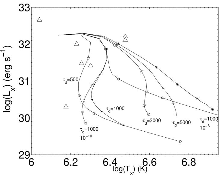
Figure 6: Evolution of the X-ray emission for a rapidly decaying fast wind as in equation 2. The value of $\tau_{d}$ is marked near each run. In all runs $\dot{M}_{1}=10^{-4}M_{\odot}~{}\rm{yr}^{-1}$, $\tau_{v}=1000~{}\rm{yr}$, and $\tau_{s}=500~{}\rm{yr}$. $\dot{M}_{\rm 2min}=10^{-9}M_{\odot}~{}\rm{yr}^{-1}$ in all cases except the one marked $10^{-10}$ and the one marked $10^{-8}$. Symbols mark 1000 yr intervals, up to 4000 yr in the run marked with diamonds, and up to 5000 yr in all other runs. All plots start at 250 yr.

The results of Fig. 6 can be interpreted as follows. As the supply of gas decreases, the hot bubble density decreases because of expansion, and thus $L_{X}$ decreases. The energy budget of the hot bubble then is dominated by adiabatic cooling. This explains why the temperatures are lower than in the previous section, although the evolution of the wind velocity $v_{2}(t)$ remained unchanged. This type of flow might result from very rapid post-AGB evolution, or if the confinement of the hot bubble by the cold shell is not perfect; For example, the two jets in NGC 40 (Meaburn et al. 1996) through which hot gas can escape, and thus reduce the X-ray temperature and luminosity.

In Fig. 7 we connect the different PNs to the nearest plot having its age equal to the dynamical age of the PN. The dynamical age of the PNs are marked on the figure. We removed three runs and added one run where we started the fast wind with $v_{20}=200~{}\rm{km}~{}\rm{s}^{-1}$, and took $\tau_{s}=1000~{}\rm{yr}$, $\tau_{d}=500~{}\rm{yr}$, $\dot{M}_{20}=10^{-6}M_{\odot}~{}\rm{yr}^{-1}$, and $\dot{M}_{1}=10^{-4}M_{\odot}~{}\rm{yr}^{-1}$ (star symbols). This figure shows that in addition to the luminosity and the temperature of the X-ray emitting gas, we can account for the age of PNs as well.

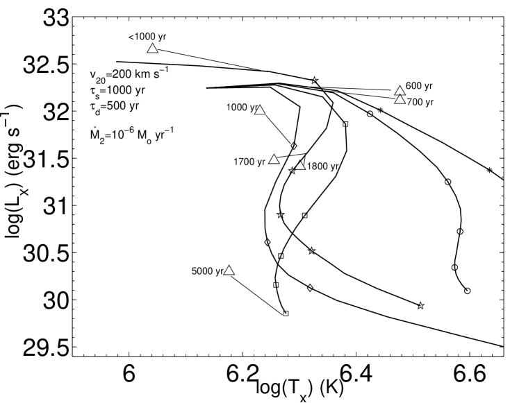
Figure 7: As Fig. 6, with three runs omitted. The dynamical age of PNs (in years)are marked, and each PN is connected to a wind age equals to its dynamical age. The stars marked a new run with parameters as written on the upper left corner.

Since we start the simulations at the PN stage, the PN time $t$ in the simulation is somewhat smaller than the actual age of the PN, by $\sim few\times 100~{}\rm{yr}$. Therefore, in Fig. 7, we connected the observed PNs to simulated $t$ values that are somewhat smaller than the observed age of the PN. For example, the upper left PN whose estimated age is 1000 yr is connected by a line to a $t=750~{}\rm{yr}$ simulation data point. We mention again that our goal is to find the general constraints on the properties of the fast wind, if it is the source of the X-ray emission, rather than to fit individual PNs. Changing a little the parameters used here, we can fit each PN individually. In addition, the composition of the fast wind also affects the X-ray properties (SS06); we use constant (solar) composition for the cooling function.

We finish this section by showing the evolution with time of the most important physical quantities. In Fig. 8 we show the evolution with time of the quantities in the run with $\dot{M}_{1}=10^{-4}M_{\odot}~{}\rm{yr}^{-1}$, $\tau_{v}=1000~{}\rm{yr}$, $\tau_{s}=500~{}\rm{yr}$, $\tau_{d}=1000~{}\rm{yr}$, and $\dot{M}_{\rm 2min}=10^{-10}M_{\odot}~{}\rm{yr}^{-1}$. The total mass lost in the fast wind (from $t=0$ in our calculation, when $v_{2}=300~{}\rm{km}~{}\rm{s}^{-1}$) at 500, 1000, and 1500 years is $\Delta M_{2}=10^{-4}M_{\odot}$, 1.387$\times 10^{-4}M_{\odot}$, and $1.4675\times 10^{-4}M_{\odot}$, respectively. Initially, the reverse (inner) shock moves outward, as does the contact discontinuity. At $t=1250~{}\rm{yr}$ it starts to move inward because the ram pressure of the fast wind decreases by a large factor. At $t=1750~{}\rm{yr}$ it starts to move outward again.

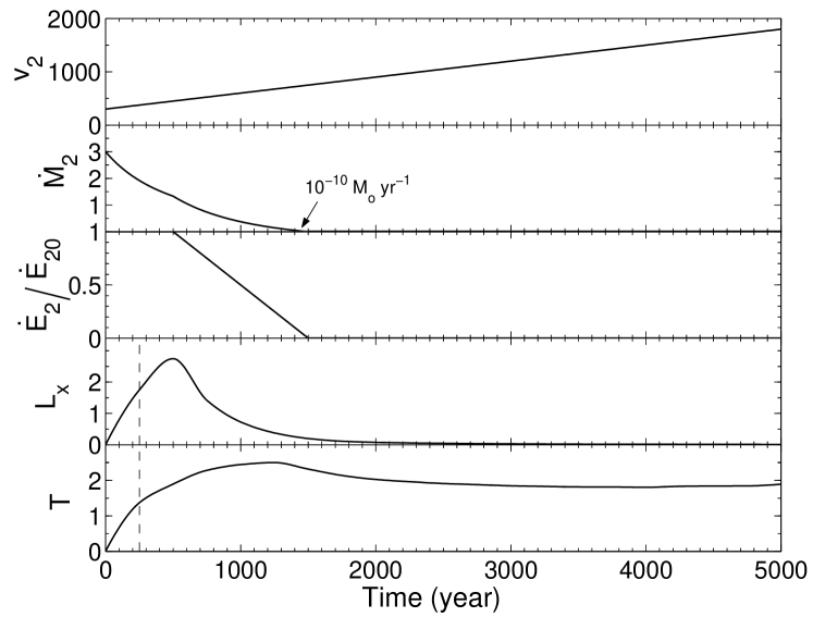
Figure 8: From top to bottom, the evolution of the fast wind speed in $~{}\rm{km}~{}\rm{s}^{-1}$, the mass loss rate in $10^{-7}M_{\odot}~{}\rm{yr}^{-1}$, the logarithm of the ratio of kinetic power to its initial value, the X-ray luminosity in $10^{-32}~{}\rm{erg}~{}\rm{s}^{-1}$ and temperature in $10^{6}~{}\rm{K}$, for the run marked by squares in Figs. 6 and 7). The first point of each run shown on Figs. 6 and 7 is at an age of 250 years, as marked here by the dashed vertical line. Note that because of radiative cooling of cooler gas, $T_{x}$ increases at late times.

5 SUMMARY

Our main finding is that if the source of the extended X-ray emitting gas in PNs is the fast wind blown by the central star, then the fast wind must be rapidly evolving. Otherwise the luminosity would be too low at early times, and the fast wind would produce hot gas at later times that is not observed. Our simulations require that the mass loss rate of the fast wind be relatively high, $\dot{M}_{2}=1-3\times 10^{-7}M_{\odot}~{}\rm{yr}^{-1}$, at early times when the wind speed is $\sim 300-700~{}\rm{km}~{}\rm{s}^{-1}$, and then it needs to rapidly decline to (Fig. 8). This weakening of the wind occurs approximately $500-1500~{}\rm{yr}$ after the fast wind has started to blow, or $\sim 1000-3000~{}\rm{yr}$ after the star has left the AGB. Our results are contradictory to those of SS06, who examined only one case of fast wind evolution, and could not find a match between their model and the X-ray properties of BD +30^∘3639 and NGC 40.

A rapid fast-wind evolution is compatible with a recent claim for rapid post-AGB evolution caused by binary interaction (Soker 2006). The high mass loss rate at the early PN phase is a continuation of a high mass loss rate during the final AGB phase. Such a high mass loss rate may lead to dust formation and strong IR emission. Montez (2006; R. Montez, private communication) suggested a correlation between IR emission and X-ray emission. Not all PNs will have such rapid fast-wind evolution, hence not all PNs will have detectable X-ray emission. Other PNs, those with slowly evolving fast winds are not expected to produce detectable X-ray emission as adiabatic cooling overcomes shock heating. Note that a slowly evolving fast wind requires a low mass loss rate. The reason is that during the post-AGB phase the mass in the envelope is very low, and the star cannot lose mass at a high rate for a long time. The low mass lose rate implies a weak X-ray emission, as the case C in Figure 5.

We should stress here that we are not claiming that all PNs owe their X-ray emission to the central star fast wind. Definitely, in some cases jets are the source of the X-ray emitting gas. If observations indicate that the fast wind evolution in PNs is much slower than required by our models, (e.g., Perinotto 2004), we will have to agree with SS06 and conclude that a central star wind can not explain the observed X-rays. Jets blown by a companion may be an alternative explanation for the X-ray emission. In this case we also expect that only a fraction of all PNs will have detectable X-ray emission. Heat conduction can also play a role, although our models show that heat conduction is not required if the fast wind evolves fast enough.

As both rapid fast-wind evolution and jets require the presence of a close companion (in the case of jets a stellar companion, in the case of rapid evolution a brown dwarf or even a massive planet might do the job as well), we propose that the extended X-ray emission in PNs is tightly connected to the presence of a close binary companion.

References

- (1)
- (2) Akashi, M., Soker, N., & Behar, E. 2006, MNRAS, 368, 1706 (ASB06)
- (3)
- (4) Arnaud, K.A., 1996, Astronomical Data Analysis Software and Systems V, eds. Jacoby G. and Barnes J., p17, ASP Conf. Series volume 101.
- (5)
- (6) Arnaud, K. , Borkowski, K. J., & Harrington, J. P. 1996, ApJ, 462, L 75
- (7)
- (8) Balick, B., & Frank, A. 2002, ARA&A, 40, 439
- (9)
- (10) Blondin J.M., 1994, The VH- 1 Users Guide, Univ. Virginia
- (11)
- (12) Blondin J.M., Kallman T.R., Fryxell B.A., Taam R.E., 1990, ApJ, 356, 591
- (13)
- (14) Cerruti-Sola, M., & Perinotto, M.1989 ApJ, 345, 339
- (15)
- (16) Chevalier, R. A. & Imamura, J. N. 1983, ApJ, 270, 554
- (17)
- (18) Chu, Y.-H., Chang, T. H., & Conway, G. M. 1997, ApJ, 482, 891
- (19)
- (20) Chu, Y.-H., Guerrero, M. A., Gruendl, R. A., Williams, R. M., Kaler, J. B. 2001, ApJ, 553, L69
- (21)
- (22) Gaetz, T. J., Edgar, R. J., & Chevalier, R. A. 1988, ApJ, 329, 927
- (23)
- (24) García-Segura, G., Lopez, J. A., Steffen, W., Meaburn, J., & Manchado, A. 2006, ApJ, Letters, in press (astro-ph/0606205)
- (25)
- (26) Gruendl, R. A., Chu, Y.-H., Guerrero, M. A., & Meixner, M. 2004, AAS, 205, 138.05
- (27)
- (28) Gruendl, R. A., Guerrero, M. A., Chu, Y.-H., & Williams, R. M. 2006 ApJ, in press (astro-ph/0607519)
- (29)
- (30) Guerrero, M. A., Gruendl, R. A, & Chu, Y.-H. 2002, A&A, 387, L1
- (31)
- (32) Guerrero, M. A., Chu, Y.-H.; Gruendl, R. A., Meixner, M. 2005, A&A, 430, L69
- (33)
- (34) Guerrero, M. A., Chu, Y.-H., Gruendl, R. A., Williams, R. M., & Kaler, J. B. 2001, ApJ, 553, L55
- (35)
- (36) Kastner, J. H., Balick, B., Blackman, E. G., Frank, A., Soker, N., Vrtilek, S. D., & Li, J. 2003, ApJ, 591, L37
- (37)
- (38) Kastner, J. H., Soker, N., Vrtilek, S. D., Dgani, R. 2000, ApJ, 545, L57
- (39)
- (40) Kastner, J. H., Vrtilek, S. D., Soker N. 2001, ApJ, 550, L189
- (41)
- (42) Leuenhagen, U., Hamann, W.-R., & Jeffery, C. S. 1996, A&A, 312, 167
- (43)
- (44) Li, J., Harrington, J. P., & Borkowski,K. J. 2002, AJ, 123, 2676
- (45)
- (46) Meaburn, J., Lopez, J. A., Bryce, M., & Mellema, G. 1996, A&A, 307, 579
- (47)
- (48) Mellema, G. 1994, A&A, 290, 915
- (49)
- (50) Moe, M., & De Marco, O. 2006, ApJ, in press
- (51)
- (52) Montez, R. Jr., Kastner, J. H., D. Marco, O., Soker, N., 2005, ApJ, 635, 381
- (53)
- (54) Murashima, M. et al. 2006, ApJ Lett. in press (astro-ph/0607144)
- (55)
- (56) Perinotto, M., Cerruti-Sola, M., & Lamers, H. J. G. L. M. 1989, ApJ, 337, 382
- (57)
- (58) Perinotto, M., Schönberner, D., Steffen, M., & Calonaci, C. 2004, A&A, 414, 993
- (59)
- (60) Sahai, R., Kastner, J. H., Frank, A., Morris, M., & Blackman, E. G. 2003, ApJ, 599, L87
- (61)
- (62) Schönberner, D., Jacob, R., & Steffen, M. 2005, A&A, 441, 573
- (63)
- (64) Schönberner, D., Jacob, R., Steffen, M., Perinotto, M., Corradi, R. L. M., & Acker, A. 2005, A&A, 431, 963
- (65)
- (66) Smith, R., K., Brickhouse, N., S., Liedahl, D., A., & Raymond, J., C. 2001, ApJL, 556, L91
- (67)
- (68) Soker, N. 1994, AJ, 107, 276
- (69)
- (70) Soker, N. 2006, ApJ, 645, L57
- (71)
- (72) Soker, N. 2004, in Asymmetrical Planetary Nebulae III: Winds, Structure and the Thunderbird, eds. M. Meixner, J. H. Kastner, B. Balick, & N. Soker, ASP Conf. Series, 313, (ASP, San Francisco), p. 562 (extended version on astro-ph/0309228)
- (73)
- (74) Soker, N. & Kastner, J. H 2003, ApJ, 583, 368
- (75)
- (76) Soker, N. & Subag, E. 2005, AJ, 130 ,2717
- (77)
- (78) Steffen, M., Schönberner, D., Warmuth, A., Schwope, A., Landi, E., Perinotto, M., & Bucciantini, N. 2005, in Planetary Nebulae as Astronomical Tools, edited by R. Szczerba, G. Stasińska, and S. K. Górny, AIP Conference Proceedings Vol. 804, (Melville, New York) 161
- (79)
- (80) Steffen, M., Szczerba, R., & Schönberner, D. 1998, A&A, 337, 149
- (81)
- (82) Stevens, I. R., Blondin, J. M., & Pollock, A. M. T. 1992, ApJ, 386, 265
- (83)
- (84) Stute, M., & Sahai, R. 2006, ApJ, in press (SS06)
- (85)
- (86) Sutherland, R.S., & Dopita, M.A. 1993, ApJS, 88, 253
- (87)
- (88) Villaver, E., Manchado, A., Garcia-Segura, G. 2002, ApJ, 581, 1204
- (89)
- (90) Volk, K. & Kwok, S. 1985, Astron. Astrophys. 153, 79
- (91)
- (92) Zhekov, S. A., & Perinotto, M. 1996, A&A, 309, 648
- (93)