X-rays from protostellar jets: emission from continuous flows

Abstract

Context. Recently X-ray emission from protostellar jets has been detected with both XMM-Newton and Chandra satellites, but the physical mechanism which can give rise to this emission is still unclear.

Aims. We performed an extensive exploration of a wide space of the main parameters influencing the jet/ambient interaction. Aims include: 1) to constrain the jet/ambient interaction regimes leading to the X-ray emission observed in Herbig-Haro objects in terms of the emission by a shock forming at the interaction front between a continuous supersonic jet and the surrounding medium; 2) to derive detailed predictions to be compared with optical and X-ray observations of protostellar jets; 3) to get insight into the protostellar jet’s physical conditions.

Methods. We performed a set of bidimensional hydrodynamic numerical simulations, in cylindrical coordinates, modeling supersonic jets ramming a uniform ambient medium. The model takes into account the most relevant physical effects, namely the thermal conduction and the radiative losses.

Results. Our model explains the observed X-ray emission from protostellar jets in a natural way. In particular we find that the case of a protostellar jet less dense than the ambient medium reproduces well the observations of the nearest Herbig-Haro object, HH 154, and allows us to make detailed predictions of a possible X-ray source proper motion ($v_{\rm sh}\approx 500$ km s^-1), detectable with Chandra. Furthermore our results suggest that the simulated protostellar jets which best reproduce the X-rays observations cannot drive molecular outflows.

1 Introduction

The early stages of the star birth are characterized by a variety of mass ejection phenomena including collimated jets. These plasma jets can travel through the interstellar medium at supersonic speed with shock fronts forming at the interaction front between the jet and the unperturbed ambient medium. In the last 50 years these features have been studied in detail in the radio, infrared, optical and UV bands and are known as Herbig-Haro (hereafter HH) objects (Herbig 1950; Haro 1952; see also Reipurth & Bally 2001).

Pravdo et al. (2001) predicted that the most energetic HH objects could be sources of strong X-ray emission. Following Zel’dovich & Raizer (1966) one can derive useful relations between the physical parameters of interest (as the plasma temperature and the shock velocity) of the post-shock region, in particular

$$T_{\rm psh}=\frac{\gamma-1}{(\gamma+1)^{2}}\left(\frac{mv_{\rm sh}^{2}}{k_{\rm B}}\right)$$ (1)

where $T_{\rm psh}$ is the post-shock temperature, $\gamma$ is the ratio of specific heats, $v_{\rm sh}$ is the shock front speed, $m$ is the mean particle mass and $k_{\rm B}$ is the Boltzmann constant. Assuming a typical velocity, $v_{\rm sh}\approx 500$ km s^-1 (as measured in HH 154, see Fridlund et al. 2005), the expected post-shock temperature is of few millions degrees, thus leading to X-ray emission.

Recently, X-ray emission from HH objects has been detected with both the XMM-Newton and Chandra satellites: the low mass young stellar objects (YSO) HH $2$ in Orion (Pravdo et al. 2001) and HH 154 in Taurus (Favata et al. 2002; Bally et al. 2003), the high mass YSO objects HH $80/81$ in Sagittarius (Pravdo et al. 2004) and HH $168$ in Cepheus A (Pravdo & Tsuboi 2005), and HH $210$ in Orion (Grosso et al. 2006). Indications of X-ray emission from protostellar jets are also discussed by Tsujimoto et al. (2004) and Güdel et al. (2005). A summary of the relevant physical quantities observed for these objects is presented in Tab. 1.

Table 1: Relevant physical quantities observed in confirmed X-ray emitting HH objects, where $L_{\rm X}$ is the reported X-ray luminosity, $kT$ and $N_{\rm H}$ are the best fit parameters derived from spectral analysis for the temperature (in keV) and for the interstellar absorption column density, $v_{\rm sh}$ is the shock front velocity derived from optical observations, $D$ is the distance of the object observed and $L_{\rm bol}/L_{\odot}$ is the bolometric luminosity of the jet driving source (Pravdo et al. 2001; Favata et al. 2002; Bally et al. 2003; Pravdo et al. 2004; Pravdo & Tsuboi 2005; Grosso et al. 2006).

object	$L_{\rm X}$	$kT$	$N_{\rm H}$	$v_{\rm sh}$	$D$	$L_{\rm bol}/L_{\odot}$	$L_{\rm X}/L_{\rm bol}$
	[$10^{29}$ erg s-1]	[keV]	[$10^{22}$ cm-2]	[km s-1]	[pc]
HH 2	$5.2$	$0.23$	$\leq 0.09$	$230$	$480$	$81$a	$1.7\times 10^{-6}$
HH 154	$3.0$	$0.34$	$1.40$	$500$	$140$	$40$b	$9.7\times 10^{-7}$
HH 80/81	$450$	$0.13$	$0.44$	$700$	$1700$	$2\times 10^{4}$c	$1.5\times 10^{-4}$
HH 168	$1.1$	$0.5$	$0.40$	$500$	$730$	$2.5\times 10^{4}$c	$3.6\times 10^{-7}$
HH 210	$10$	$0.07-0.33$	$0.80$	$130$	$450$	$-$	$-$
a Chini et al. (2001)
b Liseau et al. (2005)
c Curiel et al. (2006)

In addition to the intrinsic interest in their physics, understanding the X-ray emission from protostellar jets is important in the context of the physics of stars and planets formation. X-rays (and more in general ionizing radiation) affect many aspects of the environment of young stellar objects and, in particular, the physics and chemistry of the accretion disk and its planet-forming environment. The ionization state of the accretion disk around young stellar objects will determine its coupling to the ambient and protostellar magnetic field, and thus, for example, influence its turbulent transport. In turn, this will affect the accretion rate and the formation of structures in the disk and, therefore, the formation of planets. Also, X-rays can act as catalysts of chemical reactions in the disk’s ice and dust grains, significantly affecting its chemistry and mineralogy.

The ability of the forming star to ionize its environment will therefore significantly affect the outcome of the process, independently from the origin of the ionizing radiation. While all young stellar objects are strong X-ray sources, they will irradiate the disk from the central hole, so that stellar X-rays will illuminate the disk with grazing incidence, concentrating their effects in the central region of the disk (although flared disks can alleviate the problem to some extent). Protostellar jets are located above the disk, so that they will illuminate the disk with near normal incidence, maximizing their effects even in the outer disk regions shielded from the stellar X-rays. For example, the emission from HH 154 is located at some 150 AU from the protostar, ensuring illumination of the disk with favorable geometry out to few hundreds AU.

Several models have been proposed to explain the X-ray emission from protostellar jets, but the actual emission mechanism is still unclear. Bally et al. (2003) speculated on different mechanisms for the X-ray emission from HH 154: X-ray emission from the central star reflected by a dense medium, X-ray emission produced when the stellar wind shocks against the wind from the companion star, or produced in shocks in the jet. Raga et al. (2002) derived a simple analytic model, predicting X-ray emission originating from protostellar jets with the observed characteristics.

Prompted by this recent detection of X-ray emission from HH objects, we developed a detailed hydrodynamic model of the interaction between a supersonic protostellar jet and the ambient medium, to explain the mechanism causing the X-ray emission observed. Our model takes into account optically thin radiative losses and thermal conduction effects. We use the FLASH code (Fryxell et al. 2000) with customized numerical modules that treat optically thin radiative losses and thermal conduction (Orlando et al. 2005). The core of FLASH is based on a directionally split Piecewise Parabolic Method (PPM) solver to handle compressible flows with shocks (Colella & Woodward 1984). FLASH uses the PARAMESH library to handle adaptive mesh refinement (MacNeice et al. 2000) and the Message-Passing Interface library to achieve parallelization.

In a previous paper (Bonito et al. 2004), we presented a first set of results concerning a jet less dense than the ambient medium, with density contrast $\nu=n_{\rm a}/n_{\rm j}=10$ (where $n_{\rm a}$ is the ambient density and $n_{\rm j}$ is the density of the jet) which emits X-rays in good agreement with the X-ray emission observed in HH 154 (Favata et al. 2002). Bonito et al. (2004) have shown the validity of the physical principle on which our model is based: a supersonic jet traveling through the ambient medium produce a shock at the jet/ambient interaction front leading to X-ray emission in good agreement with observations. In the present paper, we study the effects on the jet dynamics of varying the parameters, such as the ambient-to-jet density ratio, $\nu=n_{\rm a}/n_{\rm j}$, and the Mach number, $M=v_{\rm j}/c_{\rm a}$, through a wide range, to determine the range of parameters which can give rise to X-ray emission consistent with observations. Note that we use this definition for the Mach number to be able to compare the jet velocity with the ambient sound speed, to have information on how much the jet is supersonic.

The paper is structured as follow: Sect. 2 describes the model and the numerical setup; in Sect. 3 we discuss the results of our numerical simulations; finally Sect. 4 is devoted to summary and conclusions. In Appendix  A we discuss our method to synthesize X-ray emission from our numerical simulations.

2 The model

We model the propagation of a constantly driven protostellar jet through an isothermal and homogeneous medium. We assume that the fluid is fully ionized and that it can be regarded as a perfect gas with a ratio of specific heats $\gamma=5/3$. Also we assume a negligible magnetic field.

The jet evolution is described by the fluid equations of mass, momentum and energy conservation, taking into account the effects of radiative losses and thermal conduction

$$\frac{\partial\rho}{\partial t}+\nabla\cdot\rho\mbox{\bf v}=0$$ (2)

$$\frac{\partial\rho\mbox{\bf v}}{\partial t}+\nabla\cdot\rho\mbox{\bf vv}+\nabla p=0$$ (3)

$$\frac{\partial\rho E}{\partial t}+\nabla\cdot(\rho E+p)\mbox{\bf v}=-\nabla\cdot q-n_{e}n_{H}P(T)$$ (4)

where $t$ is the time, $\rho$ the mass density, $\bf v$ the plasma velocity, $p$ the pressure, $q$ the heat flux, $n_{e}$ and $n_{H}$ are the electron and hydrogen density respectively, $P(T)$ is the optically thin radiative losses function per unit emission measure (for the P(T) we use a functional form, which takes into account: free-free, bound-free, bound-bound and 2 photons emission, see Raymond & Smith 1977; Mewe et al. 1985; Kaastra & Mewe 2000), $T$ the plasma temperature, and

$$E=\epsilon+\frac{1}{2}|\mbox{\bf v}|^{2}$$ (5)

where $E$ is the total energy and $\epsilon$ the specific internal energy. We use the equation of state for an ideal gas

$$p=(\gamma-1)\rho\epsilon\leavevmode\nobreak\ .$$ (6)

Following Dalton & Balbus (1993), we use an interpolation expression for the thermal conductive flux of the form

$$q=\left(\frac{1}{q_{\rm spi}}+\frac{1}{q_{\rm sat}}\right)^{-1}$$ (7)

which allows for a smooth transition between the classical and saturated conduction regime. In the above expression, $q_{\rm spi}$ represents the classical conductive flux (Spitzer 1962)

$$q_{\rm spi}=-\kappa(T)\nabla T$$ (8)

where $\kappa(T)=9.2\times 10^{-7}T^{5/2}$ erg s^-1 K^-1 cm^-1 is the thermal conductivity. The saturated flux, $q_{\rm sat}$, is (Cowie & McKee 1977)

$$q_{\rm sat}=-sign(\nabla T)5\phi\rho c_{\rm s}^{3}$$ (9)

where $\phi\sim 0.3$ (Giuliani 1984; Borkowski et al. 1989, and references therein) and $c_{\rm s}$ is the isothermal sound speed.

2.1 Numerical setup

We adopt a $2$-D cylindrical ($r,z$) coordinate system with the jet axis coincident with the $z$-axis. For the different cases analyzed, we have chosen different ranges for the radial and longitudinal dimensions of the computational grid to follow in all cases the jet/ambient interaction for at least 20-50 years: the computational grid size varies from $\approx 300$ AU to $\approx 600$ AU in the $r$ direction and from $\approx 6000$ AU to $\approx 3\times 10^{4}$ AU in the $z$ direction.

In the case of the jet less dense than the ambient medium (hereafter “light jet”) which best reproduces observations, the integration domain extends over $300$ AU in the radial direction and over $6000$ AU in the $z$ direction. In the case of the jet with the same initial density as the ambient medium (hereafter “equal-density jet”) which best reproduces observations, the domain is $(r\times z)\approx(600\times 6000)$ AU. In this case, the radial axis is twice as large than in the light jet case because the cocoon surrounding the equal density jet has a radial extension greater than in the light jet. The dimension of the computational domain in the case of the jet denser than the ambient (hereafter “heavy jet”) which best reproduces observations is $(r\times z)\approx(700\times 27000)$ AU.

In all the cases, the initial jet velocity is along the $z$ axis, coincident with the jet axis, and has a radial profile of the form

$$V(r)=\frac{V_{0}}{\nu\cosh(r/r_{j})^{w}-(\nu-1)}$$ (10)

where $V_{0}$ is the on-axis velocity, $\nu$ is the ambient to jet density ratio, $r_{\rm j}$ is the initial jet radius and $w\bf=4$ is the steepness parameter for the shear layer (as an example, see continuous line in Fig. 1, for the light jet case discussed in Sect. 3.2 with parameters in Tab. 3), to have a smooth transition of the kinetic energy at the interface between the jet and the ambient medium.

Figure 1: Initial jet velocity (continuous line) and density (dashed line) as a function of the distance from the axis, $r$, for the light jet case discussed in Sect. 3.2 with parameters: $M=300$, $\nu=10$, $n_{j}=500$ cm^-3, $T_{a}=10^{3}$ K, $r_{j}=30$ AU, $w=4$ (see Tab. 3).

The density variation in the radial direction (dashed line in Fig. 1) is

$$\rho(r)=\rho_{j}\left(\nu-\frac{\nu-1}{\cosh(r/r_{j})^{w}}\right)$$ (11)

where $\rho_{\rm j}$ is the jet density (Bodo et al. 1994).

Reflection boundary conditions are imposed along the jet axis, inflow boundary conditions at $z=0$ and $r\leq{r_{\rm j}}$ and outflow boundary conditions elsewhere.

The maximum spatial resolution achieved in the best light jet case, (in both $r$ and $z$ directions), is $\approx 1.3$ AU according to the PARAMESH methodology, using $4$ refinement levels, corresponding to covering the jet radius with $25$ points at the maximum resolution. The spatial resolution achieved in the equal-density case is half the one in the light jet case. In the best heavy jet model, the spatial resolution achieved is $8$ times lower than in the light jet case.

Our choice of different spatial resolution for the three cases, aimed at reducing computational cost, was necessary because the thermal conduction is solved explicitly in FLASH and, therefore, a time-step limiter depending on density, $\rho$, temperature, $T$, and spatial resolution, $\Delta x$, is required to avoid numerical instability (see, for instance, Orlando et al. 2005). Stability is guaranteed for $\Delta t<0.5\leavevmode\nobreak\ \Delta x^{2}/D$, where $D$ is the diffusion coefficient, related to the conductivity, $\kappa$, and to the specific heat at constant volume, $c_{v}$, by $D=\kappa(T)/(\rho c_{v})$. In models characterized by high values of temperature (as, for instance, in the heavy jet case), therefore, a lower spatial resolution was required to avoid a very small time-step, $\Delta t$.

2.2 Time scales

Condensations of plasma, due to radiative cooling effects, can become thermally unstable; however the presence of thermal conduction can prevent such instabilities. By comparing the radiative, $\tau_{\rm rad}$, and thermal conduction, $\tau_{\rm cond}$, characteristic times

$$\tau_{\rm rad}=\frac{p}{(\gamma-1)n_{e}n_{H}P(T)}\approx 2.5\times 10^{3}\frac{T^{3/2}}{n}$$ (12)

$$\tau_{\rm cond}\approx\frac{p}{\gamma-1}\frac{7}{2}\frac{l^{2}}{\kappa(T)T}\approx 1.5\times 10^{-9}\frac{nl^{2}}{T^{5/2}}\leavevmode\nobreak\ ,$$ (13)

where $l$ represents the characteristic length of temperature variations, we can infer which of the two competing processes dominates during the jet/ambient interaction. From the condition

$$\left(\frac{\tau_{\rm rad}}{\tau_{\rm cond}}\right)^{1/2}=1$$ (14)

we can derive the cutoff length scale for instability, $l_{\rm F}$ (Field 1965), which indicates the maximum length

$$l_{\rm F}\approx 1.3\times 10^{6}\frac{T^{2}}{n}$$ (15)

over which thermal conduction dominates over radiative effects,in the classical conduction regime. An analogous estimate in the saturation regime leads to

$$\left(l_{\rm F}\right)_{\rm sat}\approx 3\times 10^{7}\frac{T^{2}}{n}\leavevmode\nobreak\ ,$$ (16)

which is one order of magnitude longer than the characteristic length in the classical regime. As discussed later in Sect. 3.2, the comparison between the classical Field length (the shortest characteristic length) and the size of the region behind the shock at the head of the jet will allow us to determine if this region is thermally stable or not.

In order to verify our hypothesis of a fully ionized gas, we computed the ionization time scale of the most relevant elements in the X-ray spectrum of a shocked plasma at $T=3.4\times 10^{6}$ K, assuming a post-shock density of about $10^{4}$ cm^-3 (the light jet case). As an example, we derived that the ionization time scale for C and O is 1 to 2 orders of magnitudes smaller than the radiative and thermal conduction time scales so that the plasma can be considered in equilibrium.

2.3 Parameters

Our model solutions depend upon several physical parameters as, for instance, the jet and ambient temperature and density, the jet velocity and its radius. With the aim to reduce the number of free parameters in our exploration of the parameter space, we fixed the jet radius to $r_{j}\approx 30$ AU, according to Favata et al. (2002) who found this characteristic linear scale, from the X-ray thermal fit, and according to Fridlund et al. (2005) who showed HST images of the internal knots of HH 154 with dimension $r\approx 30$ AU at the base of the jet. However detailed simulations with different $r_{j}$ values are not necessary since we can predict the effects of varying the jet radius from the model results we obtained so far. In fact we expect the X-ray emitting region to grow in size as $r_{j}$ grows. Since the X-ray luminosity is defined as $L_{\rm X}=n^{2}VP(T)$, it depends on the cube of the radius. This means that, $L_{\rm X}$ being constrained from observations, a jet with a greater radius needs a lower density in order to reproduce observations. We impose an initial jet length $z_{j}=300$ AU to avoid the ejected plasma that travels back inside the boundary during the jet evolution. This choice of a non-zero initial jet length allows us to obtain an unperturbed boundary surface at $z=0$. In all our simulations, we model a jet with initial density and temperature $n_{\rm j}=500$ cm ^-3 and $T_{\rm j}=10^{4}$ K respectively, according to the values derived from observations (Fridlund & Liseau 1998 and Favata et al. 2002). The density and temperature of the ambient medium, $n_{\rm a}$ and $T_{\rm a}$ respectively, are derived from the choice of the ambient-to-jet density contrast, $\nu$ and from the hypothesis of initial pressure balance between the ambient medium and the jet. We are left, therefore, with two non-dimensional control parameters: the jet Mach number, $M$, and the ambient-to-jet density contrast, $\nu$. For a more extended exploration of the parameter space, see Sect. 3.5, concerning the variation of the initial jet density, $n_{\rm j}$. In our simulations we account for a wide jet/ambient parameters range shown in Tab. 2.

Table 2: Range of parameters used in our numerical model (column 2) compared with typical outflow parameters (column 3 and 4) shown in Bally & Reipurth (2002), Tab. 1. $\nu$ is the ambient to jet density contrast; $M$ is the Mach number; $T_{a}$ and $n_{a}$ are the ambient temperature and density, respectively; $v_{\rm j}$ is the initial jet velocity; $v_{\rm sh}$ is the shock velocity of the knots inside the jet; $\dot{M}$ is the mass loss rate; $L_{\rm mech}$ is the mechanical luminosity.

Parameter	Model	Low Massa	High Massa	Units
$\nu$	$0.01\div 300$	$-$	$-$	$-$
$M$	$1\div 1000$	$-$	$-$	$-$
$T_{a}$	$30\div 10^{6}$	$-$	$-$	K
$n_{a}$	$5\div 10^{5}$	$-$	$-$	cm-3
$v_{\rm j}$	$85\div 8500$	$-$	$-$	km s-1
$v_{\rm sh}$	$100\div 2000$	$100\div 300$	$100\div 1000$	km s-1
$\dot{M}$	$10^{-10}\div 10^{-8}$	$10^{-9}\div 10^{-5}$	$10^{-6}\div 10^{-2}$	$M_{\odot}$ yr-1
$L_{\rm mech}$	$6.7\times 10^{-5}\div 67$	$0.001\div 1$	$0.1\div 1000$	$L_{\odot}$
a Bally & Reipurth (2002)

In Sect. 3, we discuss the results derived from the exploration of the parameters space defined by $M$ and $\nu$.

3 Results

3.1 Exploration of the parameter space

We performed a wide exploration of the parameter space defined by two free parameters: the jet Mach number, $M=v_{\rm j}/c_{\rm a}$, and the ambient-to-jet density ratio, $\nu=n_{\rm a}/n_{\rm j}$ (see Sect. 2.3). The aim is to determine the range of parameters leading to X-ray emission from protostellar jets in agreement with the observations.

We first analyzed adiabatic hydrodynamic models, i.e. without thermal conduction and radiative losses. Then, for the most promising cases (i.e. those which reproduce the values of jet velocity, temperature and luminosity of the X-ray source derived from the observations), we performed more realistic simulations in which we have taken into account thermal conduction and radiative losses effects. By comparing these models with those without thermal conduction and radiative cooling, we explored how the presence of these physical processes affects the jet/ambient system evolution. We found that, in general, models with thermal conduction and radiation reach lower temperatures (up to $5$ times lower than those achieved in the adiabatic cases). We also found that thermal conduction smooths the structures (well visible in the pure hydrodynamic cases) in the density and temperature distributions.

In the following subsections, we discuss the models (shown in Fig. 2) in which both radiative losses and thermal conduction are taken into account. In Fig. 2 green and red dots refer to those cases with X-ray luminosity $L_{X}>10^{28}$ erg s^-1, shock front velocity $v_{sh}>100$ km s^-1 and fitting temperature $T<10^{7}$ K, consistent with observations. We have chosen $L_{X}$ one order of magnitude lower than the minimum value observed (see Tab. 1) to take into account fainter sources not detected so far; the red dot refers to the representative case of HH 154 discussed in Bonito et al. (2004). Squares show cases with velocity in the range of values observed, but with $L_{X}<10^{28}$ erg s^-1. Diamonds mark the cases with velocity and X-ray luminosity not consistent with observations. Triangles mark cases with temperatures higher than $10^{7}$ K. The lower panel of Fig. 2 show the initial velocity assumed in our simulations vs. the density contrast.

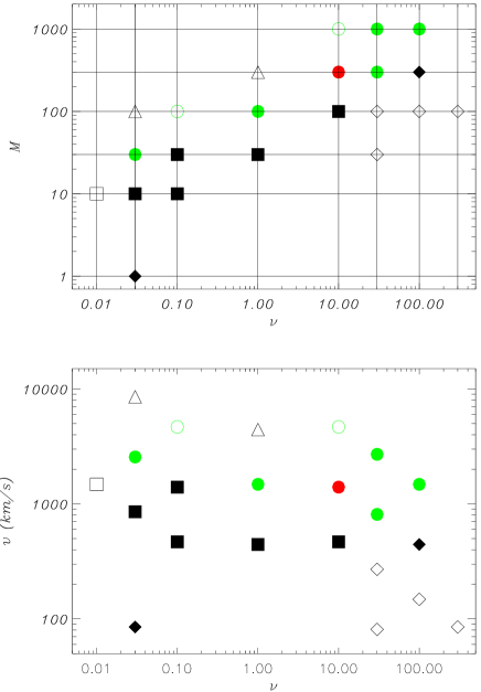
Figure 2: Exploration of the parameter space: jet Mach number, $M$ (upper panel) and initial jet velocity (lower panel) as a function of the ambient-to-jet density contrast, $\nu$. Green and red dots refer to models consistent with observations for X-ray luminosity, shock velocity and fitting temperature values (see text); diamonds refer to models which cannot reproduce observations; squares refer to models in good agreement with observations for shock velocity but not for X-ray luminosity values; triangles refer to models with too high ($T\geq 10^{7}$ K, one order of magnitude higher than observed) temperature. Empty symbols refer to pure hydrodynamic simulations; filled symbols refer to models in which thermal conduction and radiative losses effects are taken into account.

From our exploration of the parameter space, we derived that the models in agreement with observations are included in a well constrained region. In the following sections, we discuss in details the “best-fit” models, i. e. those models which reproduce X-ray luminosity and shock front speed values as close as possible to those observed, in the cases of light, equal-density and heavy jets (see Tab. 3).

Table 3: Summary of the initial physical parameters characterizing the “best-fit” models in the cases of light, equal-density and heavy jets: ambient-to-jet density contrast, $\nu$, jet Mach number, $M$, initial jet velocity, $v_{\rm j}$, ambient density and the temperature, $n_{\rm a}$, and $T_{\rm a}$, respectively. In all the models, the initial jet density and temperature are $n_{\rm j}=500$ cm ^-3 and $T_{\rm j}=10^{4}$ K, respectively.

model	$\nu$	$M$	$v_{\rm j}$	$n_{\rm a}$	$T_{\rm a}$
			[km s-1]	[cm-3]	[$10^{4}$ K]
light	10	300	1400	5000	0.1
equal-density	1	100	1500	500	1
heavy	0.03	30	2500	17	30

3.2 Hydrodynamic evolution

In Fig. 3, we show the mass density and temperature distributions $20$ years since the beginning of the jet/ambient medium interaction for the three best-fit models in Tab. 3. The light jet case is the one which better reproduce the physical parameters derived from observations by Fridlund & Liseau (1998) and Favata et al. (2002) for the HH 154 protostellar jet; its properties have been discussed in Bonito et al. (2004).

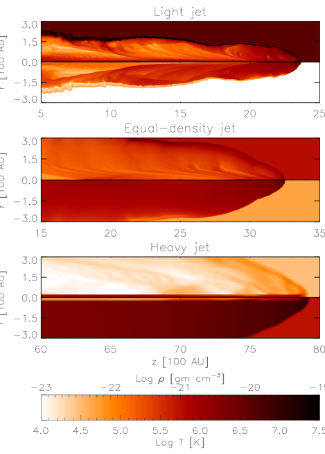
Figure 3: Mass density (upper semi-panels) and temperature (lower semi-panels) bi-dimensional cuts in the $r-z$ plane after $20$ years since the beginning of the jet/ambient interaction for the best cases of light (upper panels), equal-density (middle panels) and heavy jet (lower panels).

In all the cases, at the head of the jet there is clear evidence of a shock front due to the plasma propagating supersonically along the jet axis. Just behind the shock front there is a localized hot and dense blob (see, for instance, the enlargement in Fig. 4 for the light jet case).

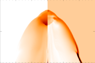
Figure 4: An enlargement of the post shock region in the light jet case of temperature (left) and density (right) in linear scale, about $20$ years since the beginning of the jet/ambient interaction. Note the hot and dense region just behind the shock front.

The light jet is enveloped by a cocoon with temperature $T\approx 7\times 10^{5}$ K, almost uniform due to the thermal conduction diffusive effect; nevertheless the cocoon temperature is not constant in time but decreases as the evolution goes on, leading to the formation of a cool and dense external envelope. Fig. 5 shows cuts of the density (continuous line) and temperature (dashed line) along the radius at $z\approx 5000$ AU, corresponding to the blob position 40 years since the beginning of the jet/ambient interaction: the hot (few millions degrees) and dense blob is evident for $r<10$ AU. The density decreases moving away from the jet axis along the radial direction and, then, it increases again at the position corresponding to the external part of the cocoon. On the other hand, the temperature monotonously decreases, moving away from the jet axis along the radial direction. The blob, therefore, is expected to be an X-ray source; in Sect. 3.4.2, we will show that the X-ray source has luminosity and spectral characteristics consistent with those observed.

Figure 5: Density (continuous line) and temperature (dashed line) profile along the radial direction at $z\approx 5000$ AU corresponding to the blob position at $t=40$ yr ($M=300$, $\nu=10$).

The central panel in Fig. 3 shows 2-D sections in the $(r,z)$ plane of the mass density and temperature distributions for the best-fit equal-density model (see Tab. 3). The interaction between the protostellar jet and the ambient medium causes the presence of a dense and hot cocoon ($n\approx 1400$ cm^-3; $T\approx 2\times 10^{6}$ K) surrounding the jet. Once again the cocoon is almost uniform for the presence of the thermal conduction but its temperature decreases with time. The cocoon becomes gradually cool and dense with time as in the light-jet case. Also in this case, the post-shock region is a hot and dense blob from which the X-ray emission originates (see Sect. 3.4.1 for more details).

In the heavy-jet case (lower panel in Fig. 3), the jet is surrounded by a cocoon well smoothed by the effects of the thermal conduction and with a radial extension larger than in the other two cases. The cocoon has temperature of a few millions degrees and density lower than that of the jet.

For the three best-fit models discussed above, we analyzed the thermal stability of the hot and dense blob localized behind the shock by comparing the size of the blob with the Field length Eq. 15. In the light jet case, the values obtained for the average blob temperature, $T\approx 3.4\times 10^{6}$ K, and density, $n\approx 6500$ cm^-3, lead to $l_{\rm F}\sim 100$ AU. Since the blob size, almost equal to twice the initial jet radius $r_{\rm j}\approx 30$ AU (see Fig. 4), is smaller than $l_{\rm F}$, it turns out that the blob is thermally stable. In the equal-density jet case, the density and temperature of the blob at the head of the jet are $n\approx 1700$ cm^-3 and $T\approx 4.3\times 10^{6}$, respectively, leading to $l_{\rm F}\approx 10^{3}$ AU. Also in this case, therefore, the blob is thermally stable, being its size $\sim 100$ AU, i.e. $10$ times smaller than the Field length. In the heavy-jet case, the temperature and density of the blob are $T\sim 10^{7}$ K and $n\sim 10^{2}$ cm^-3, leading to $l_{\rm F}\approx 10^{4}$ AU. Since the blob behind the shock front extends over about $100$ AU, also in this case it is thermally stable.

Figure 6: Shock front position vs. time. Dots mark the light jet case, stars the equal-density jet and crosses the heavy jet case. The lines refer to the best-fit from which we derive the average shock speed: $v_{\rm sh}\approx 500$ km s^-1, $\approx 600$ km s^-1, $\approx 1900$ km s^-1 for the light, equal-density and heavy jet case, respectively.

The position of the shock front as a function of time for the three best-fit models in Tab. 3 is shown in Fig. 6. For the light jet case, we derived an average shock velocity $v_{\rm sh}\approx 500$ km s^-1, about $3$ times lower than the initial jet velocity. This shock velocity is in good agreement with observed speeds in HH objects and in particular with that derived from HH 154 data. Taking into account the jet inclination $\approx 45$ degrees (Fridlund & Liseau 1998), $v_{\rm sh}\approx 500$ km s^-1 corresponds to a proper motion of $\approx 350$ km s^-1, which, at the distance of HH 154, can be measured with well time-spaced Chandra observations.

In the equal-density jet scenario, we deduced an average shock velocity $v_{\rm sh}\approx 600$ km s^-1, slightly greater than the value observed in HH 154 (Fridlund & Liseau 1998; Favata et al. 2002), but consistent with values observed in other HH objects (see Tab. 1). For the heavy jet case, the average value of the shock speed is $v_{\rm sh}\approx 1900$ km s^-1 which is too high with respect to the HH shock front velocities observed (cf. Tab. 1).

3.3 Emission measure distribution vs. temperature

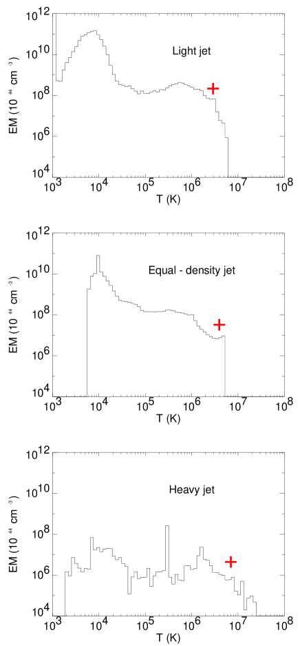
Figure 7: Emission measure, $EM$, as a function of the temperature, $T$ for the three models discussed, $20$ years since the beginning of the jet/ambient interaction. The cross superimposed on each panel marks the best-fit temperature and emission measure values derived from our simulated absorbed spectra.

We derived the distribution of emission measure vs. temperature, $EM(T)$, in the temperature range [$10^{3}-10^{8}$] K at different stages of the evolution of the jet/ambient system (see Appendix A for more details). Fig. 7 shows the $EM(T)$ for the three best-fit models in Tab. 3, after $20$ years since the beginning of the jet/ambient interaction.

In all the cases, we found that the shape of the $EM(T)$ is characterized by two bumps, and does not change significantly during the system evolution. The relative weight of the bumps is different in the three cases. In the light jet case (upper panel in Fig. 7), the bumps are quite broad, the first centered at temperature $T\sim 10^{4}$ K with $EM\sim 10^{55}$ cm^-3, and the second one centered at $T\sim 10^{6}$ K with $EM\sim 10^{52}$ cm^-3, about three orders of magnitude lower than the previous one; the $EM$ decreases rapidly above few millions degrees.

In the equal-density jet case (middle panel in Fig. 7), the first bump is centered at $T\sim 10^{4}$ K with $EM\geq 10^{54}$ cm^-3, whereas the second bump is centered at $T\sim 10^{6}$ K with $EM\sim 10^{52}$ cm^-3, as in the light jet case. In the heavy jet case (lower panel in Fig. 7), the $EM(T)$ distribution appears flat with two weak peaks: the first centered at $T\sim 10^{4}$ K and the second one at a few millions degrees. Note that, in the heavy jet case, the EM at temperature up to a few million degrees is two orders of magnitude lower than in the light jet case.

On the base of the $EM(T)$ distribution, we expect a bright ($L_{\rm X}>10^{28}$ erg s^-1) X-ray source, whose soft component (due to the cocoon) could be suppressed by the strong interstellar medium absorption (Favata et al. 2002). We expect also that the X-ray emission decreases as the ambient-to-jet density ratio, $\nu$, decreases, leading to a brighter X-ray emission in the light jet case.

3.4 X-ray emission

From the $EM(T)$ distributions and the MEKAL spectral code, we synthesized the focal plane spectra as predicted to be detected with the instruments on board XMM-Newton and Chandra (see Appendix A for details), taking into account the interstellar absorption. To compare our numerical models with experimental data concerning HH 154 (the closest and best studied jet emitting in the X-ray band), we assumed a distance of 150 pc (as HH 154 that is located in the L1551 cloud in the Taurus star-forming region) and an interstellar absorption column density $N_{\rm H}=1.4\times 10^{22}$ cm^-2 (Favata et al. 2002). Our model results can be generalized to account for the other HH objects observations by considering different values for the distance and the interstellar absorption.

3.4.1 Spatial distribution of the X-ray emission

Assuming the jet propagating perpendicularly to the line of sight, from the numerical simulations we derived X-ray images of the jet/ambient system as predicted to be observed with Chandra/ACIS-I (see Appendix A) that allows us to pinpoint the X-ray emission, thanks to its high spatial resolution. For all the models in Tab. 3, we derived the evidence that most of the X-ray emission produced during the jet/ambient medium interaction originates from a very compact region localized at the head of the jet, just behind the shock front.

Fig. 8 shows an enlargement of the X-ray images as predicted to be detected with Chandra/ACIS-I of the head of the jet where most of the X-ray emission originates, 20 years since the beginning of the jet/ambient interaction. Note that the spatial resolution of the X-ray images in Fig. 8 is 6 times better than that of Chandra/ACIS-I. In all the three cases analyzed, a comparison between the X-ray emitting region and the temperature and density maps in Fig. 3 shows that the X-ray source is coincident with the hot and dense blob discussed in Sect. 3.2.

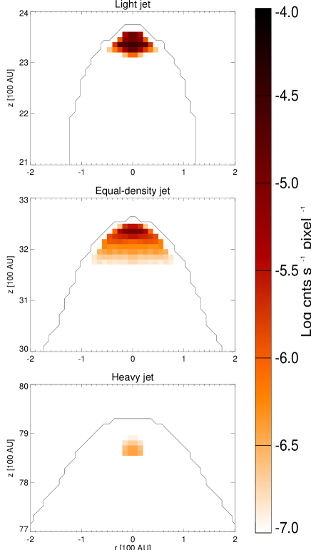
Figure 8: Synthesized X-ray emission, in logarithmic scale, as observed with ACIS-I, for the three cases examined, $20$ years since the beginning of the jet/ambient interaction. At a distance $D\approx 150$ pc, 100 AU correspond to about 0.7 arcsec

We found that even with Chandra’s spatial resolution, the X-ray emitting region cannot be spatially resolved (the spatial resolution of the synthesized X-ray images in Fig. 8 is 6 times better than that of Chandra), and it will be detected as a point-like source. Also, significant X-ray emission is visible only from the hot and dense blob behind the shock front, as softer cocoon emission is extinguished by the the strong interstellar absorption.

As discussed in Sect. 3.2, the X-ray emitting region for the three cases examined is thermally stable, and therefore the X-ray emission is detectable continuously during the 20-50 years analyzed. We found also that there are no significant variations of the X-ray source morphology during the evolution: the source size varies by $\pm 25\%$, always below the spatial resolution achievable with Chandra, and there is no disappearance of the X-ray emitting region, according to the stability analysis. On the other hand, for some of the cases shown in Fig. 2, our analysis predicts a transient behaviour of the X-ray source, which extinguishes, few years since the beginning of the interaction between the protostellar jet and the ambient medium, because of the radiative cooling which dominates over the thermal conduction effects.

From Fig. 6, the X-ray source, coincident with the hot and dense blob discussed in Sect. 3.2, has a proper motion of $\sim 0.7$ arcsec/yr, $\sim 0.8$ arcsec/yr, and $\sim 2.7$ arcsec/yr in the light, equal-density and heavy jet case respectively, assuming the jet axis to be perpendicular to the line of sight. In addition, we found that the intensity of the X-ray source decreases about one order of magnitude as the ambient-to-jet density contrast, $\nu$, decreases. Note that the heavy jet case has the higher shock front speed and the lower X-ray emission.

3.4.2 Spectral analysis

We derived the synthesized focal plane spectra as they would be detected with XMM-Newton/EPIC-pn, characterized by an high effective area, with the aim to compare our model results with published data and, in particular, with those concerning HH 154 (Favata et al. 2002).

We considered two different levels of count statistics in the $[0.3-10]$ keV band: in the low statistics case we have chosen an exposure time so as to obtain about $100$ total photons for each spectrum whereas, in the high statistics case, we imposed about $10^{4}$ counts for each spectrum. Albeit the latter case is unrealistic, given the low photon counts so far collected from these sources, it can help us to pinpoint some fundamental features of the predicted spectra. The spectral bins are grouped together to have at least 10 photons in the low count statistics case and 20 photons in the other case.

For the models of light and equal-density jet, the synthesized spectra are well described as the emission from an optically thin plasma at a single temperature, even in the high count statistics case. This result is due to the strong interstellar absorption which suppresses the soft emission originating from the cooler plasma component in the cocoon. The best fit parameters derived from our simulations are shown in Tab. 4.

Table 4: Best-fit parameters for the EPIC-pn simulated X-ray spectra obtained in the low and high statistics cases, respectively, for the three best-fit models of Tab. 3, about 20 yr since the beginning of the jet/ambient interaction.

Model	counts	$N_{\rm H}\pm\Delta N_{\rm H}$	$T_{1}\pm\Delta T_{1}$	$EM_{1}\pm\Delta EM_{1}$	$T_{2}\pm\Delta T_{2}$	$EM_{2}\pm\Delta EM_{2}$	$\chi^{2}$	Prob.a
		$(10^{22}$ cm${}^{-2})$	($10^{6}$ K)	($10^{52}$ cm${}^{-3})$	($10^{6}$ K)	($10^{52}$ cm${}^{-3})$
Light	102	$1.4\pm 0.3$	$2.9\pm 1.2$	$2.5\pm 10.9$	$-$	$-$	0.44	0.88
	10317	$1.39\pm 0.02$	$2.9\pm 0.1$	$2.2\pm 0.6$	$-$	$-$	0.73	1.00
Equal-density	71	$1.3\pm 0.4$	$3.1\pm 3.8$	$0.4\pm 3.5$	$-$	$-$	0.49	0.75
	10134	$1.38\pm 0.02$	$3.9\pm 0.2$	$0.33\pm 0.09$	$-$	$-$	0.72	1.00
Heavy	92	$1.4\pm 0.2$	$6.8\pm 1.7$	$0.9\pm 3.4$	$-$	$-$	0.39	0.93
	9811	$1.40\pm 0.04$	$3.0\pm 0.1$	$0.2\pm 0.2$	$11.8\pm 0.4$	$0.016\pm 0.002$	0.73	0.99
a Null hypothesis probability.

The heavy jet model which best fits HH observations show more structured spectra than those obtained in the light jet and equal-density jet cases: in the high statistics case, the spectra are well described by a two temperature plasma emission, with the best fit parameters reported in Tab. 4.

The spectral analysis reflects the structure of the $EM(T)$ distribution: the spectra are sensitive to the high temperature portion of the $EM(T)$ (see Fig. 7), being the softer component suppressed by the interstellar medium absorption. On the other hand, in the heavy jet model, the $EM(T)$ distribution is characterized by a bump at high temperatures broader than those in the other two cases (see Fig. 7), implying that more than a single temperature contributes to the emission.

Fig. 9 shows the evolution of the X-ray luminosity, $L_{\rm X}$, in the $[0.3-10]$ keV band, derived from the isothermal components fitting the spectra in the high statistics case. The light jet case (dots in Fig. 9) shows $L_{\rm X}$ values in good agreement with those observed in HH 154 ($L_{\rm X}=3\times 10^{29}$ erg s^-1, see Favata et al. 2002). In the equal-density jet case, $L_{\rm X}$ ranges between $7.4\times 10^{28}$ and $2.7\times 10^{29}$ erg s^-1, in general below the luminosity observed in HH 154, although its values are consistent with those detected in other HH objects (see Tab. 1). On the other hand, in the heavy jet case, the $L_{\rm X}$ values (crosses in Fig. 9) are at least one order of magnitude lower than those observed so far in HH objects (Tab. 1) and in HH 154 in particular.

Figure 9: X-ray luminosity evolution as a function of time. Dots mark the light jet case, stars the equal-density jet and crosses the heavy jet case. The line superimposed on this figure marks $L_{\rm X}=3\times 10^{29}$ erg s^-1, the value observed in HH 154 (Favata et al. 2002).

3.5 Varying the jet density parameter

As an extension of the exploration of the parameter space, we have varied the value of the initial jet density, $n_{\rm j}$, so far fixed to the value derived from Fridlund & Liseau (1998) for HH 154 (namely $n_{\rm j}=500$ cm^-3). In particular, we performed the numerical simulation of a jet with initial density $n_{\rm j}=5000$ cm^-3, ten times denser than the ambient medium ($\nu=0.1$), and with Mach number $M=20$, corresponding to an initial jet velocity $v_{\rm j}\approx 950$ km/s. We found that this model is thermally unstable since the size of the X-ray emitting region at the head of the jet is larger than the corresponding characteristic Field length. As a consequence, the X-ray luminosity initially at values $\approx 3\times 10^{29}$ erg/s drops of over $2$ orders of magnitude in about $10$ years.

Higher values of the X-ray emission could be obtained in cases with: 1) higher initial jet density, $n_{\rm j}$; 2) higher ambient-to-jet density contrast, $\nu$; 3) higher initial jet velocity, $v_{\rm j}$.

To account for the first option (higher $n_{\rm j}$), we performed the same numerical simulation discussed above, but with initial jet density $10$ times greater, namely $n_{\rm j}=5\times 10^{4}$ cm^-3. In this case, we derived shock front velocity $\approx 800$ km/s and X-ray luminosity ranging between $3$ and $30\times 10^{29}$ erg/s and emission consistent with HH observation in general, but too high to reproduce the observations of HH 154. Such initial jet density adopted turns out to be much higher than those derived from observations of HH objects. Podio et al. (2006) studied several HH objects and derived principal physical properties as their density. In particular they found that the density ranges between $400$ and $1000$ cm^-3 (see also Fridlund & Liseau 1998 for density values in HH 154).

As it concerns the second and third options discussed above, based on our exploration of the parameter space Fig. 2, we expect that for fixed initial jet velocity, the X-ray luminosity increases with increasing $\nu$ and vice versa. Again we conclude that the jet must be less dense than the ambient medium and/or with initial jet velocity higher than $950$ km/s. Once again our analysis leads to the conclusion that X-ray emission originating from protostellar jets (in particular from HH 154) is better reproduced by light jets with initial jet density $n_{\rm j}=500$ cm^-3.

4 Discussion and conclusions

We presented an hydrodynamic model which describes the interaction between a supersonic protostellar jet and a homogeneous ambient medium. The aim is to derive the physical parameters of a protostellar jet which can give rise to X-ray emission consistent with the recent observations of HH objects.

In a previous paper (Bonito et al. 2004), we have shown the feasibility of the physical principle on which our model is based: a supersonic protostellar jet leads to X-ray emission from the shock, formed at the interaction front with the surrounding gas, consistent with the observations in the particular case of HH 154, the nearest and best studied X-ray emitting protostellar jet. Here we have performed an extensive exploration of a wide space of those parameters which mainly describe the interaction of the jet/ambient system: the jet Mach number, $M$, and the ambient-to-jet density contrast, $\nu$ (Fig. 2). These results, therefore, provide insight in a wider set of phenomena, allowing us to study and diagnose physical properties of protostellar jets in general, other than that in L$1551$.

One of the main results of our analysis is that only a narrow range of parameters can reproduce observations. The extensive exploration of the parameter space here discussed improves and extends the previous work by allowing us to constrain the main protostellar jets parameters in order to obtain X-ray emission, best fit temperature and shock front speed consistent with experimental data.

The range of parameters which more significantly influences the jet/ambient evolution are shown in Tab. 2. From a comparison with observed quantities (also shown in Tab. 2, according to Bally & Reipurth 2002) it can be deduced that the parameters used in our model are consistent with observed values. Note that the values of initial jet velocity are higher than the observed values. This apparent discrepancy is due to the fact that observers measure the velocity of the knots which have already been slowed down by the interaction with the ambient medium. So we need a higher initial jet velocity to account for these lower speed values at the working surface. However in the best light jet case, we derive a kinetic power $L_{\rm mech}\approx 0.3$ $L_{\odot}$, more than 2 orders of magnitude lower than the observed bolometric luminosity of HH $154$, $L_{bol}\approx 40$ $L_{\odot}$ (see Tab. 1). So the jet velocity values used in our simulations lead to reasonable kinetic power. Furthermore comparing the X-ray luminosity derived in the best light jet model here discussed, we deduce that only a small fraction of the kinetic power is converted in X-ray emission: $L_{X}/L_{\rm mech}\approx(8\times 10^{-5}$ $L_{\odot})/(0.3$ $L_{\odot})=3\times 10^{-4}$.

In the following we summarize our findings:

• Light jet ($\bf\nu>1$).
  The light jet cases which reproduce the X-ray emission and optical proper motion observed are those with initial Mach number $M\geq 300$ and ambient-to-jet density contrast $10\leq\nu<100$. For Mach numbers lower than $M=300$, the X-ray luminosity derived from our simulations is lower than the minimum value observed in protostellar jets ($(L_{\rm X})_{\rm obs}>10^{28}$ erg s^-1) and, in some cases, with a transient behaviour due to thermal instabilities. The values $M=300$ and $\nu=10$ provide the best case which reproduces the HH 154 observations in terms of best fit temperature, emission measure and X-ray luminosity. We also predict a substantial proper motion.

• Equal-density jet ($\bf\nu=1$).
  The three equal-density jet cases analyzed allow us to constrain the initial Mach number of an equal-density protostellar jet to reproduce observations: $30<M<300$. From the equal-density model with $M=100$ we derive shock front velocity and X-ray luminosity consistent with HH objects observations in general (see Tab. 1).

• Heavy jet ($\bf\nu<1$).
  To reproduce some characteristics of the observations, in the heavy jet scenario, we need initial jet Mach number $M\approx 30$ and initial jet density much higher than the ambient density, $\nu\leq 0.03$, i.e. a jet $30$ times denser than the medium or more. Lower initial Mach number in some cases leads to thermal instability which suppress X-ray emission about $5$ years since the beginning of the interaction between the protostellar jet and the ambient medium. A jet $30$ times denser than the ambient medium ($\nu=0.03$) and with initial Mach number $M=30$ predicts emission from a million degrees plasma. Although its $v_{\rm sh}$ is too high and its $L_{\rm X}$ is too low with respect to those observed in HH objects in general (see Tab. 1) and in HH 154 in particular (Favata et al. 2002), we cannot reject the possibility of new more sensitive observations which may show fainter emission not yet detected in X-ray emitting HH objects.

Here we discussed the best-fit models of light, heavy and equal-density jets in best agreement with experimental results from HH objects in general: a light jet with $M=300$ and $\nu=10$; an equal-density jet with $M=100$ and $\nu=1$; and a heavy jet with $M=30$ and $\nu=0.03$.

For each case, we analyzed the evolution of the mass density and temperature spatial distributions derived from our model, the shock front proper motion and its spectral properties, the X-ray emission and its stability. In each best-fit model the interaction between the supersonic protostellar jet and the unperturbed ambient medium leads to the formation of a hot and dense cocoon surrounding the jet and smoothed by the thermal conduction. Just behind the shock front, there is a hot and dense blob from which the harder and bright X-ray emission originates: the strong interstellar absorption suppresses the softer component due to the cocoon. In all cases examined, the X-ray emitting region is thermally stable, i.e. thermal conduction effects prevent the collapse of the source due to radiative cooling, and shows a detectable proper motion.

To compare our findings with HH 154 observations, we have rejected any equal-density and heavy jet case which show too high shock front velocity ($v_{\rm sh}\approx 600$ km s^-1 and $\approx 1900$ km s^-1, respectively) and too low X-ray luminosity ($L_{\rm X}\approx 10^{29}$ erg s^-1 and $\approx 10^{28}$ erg s^-1) with respect to $v_{\rm sh}$ and $L_{\rm X}$ values observed in HH 154 ($v_{\rm sh}\approx 500$ km s^-1 and $L_{\rm X}=3\times 10^{29}$ erg s^-1).

In the best light jet case, we derived a particle density $n\approx 6500$ cm^-3 and a velocity $v_{sh}\approx 500$ km s^-1 for the X-ray emitting region, leading to a momentum $mv=2\times 10^{-6}$ $M_{\odot}$ km s^-1. This value is consistent with the upper limit $7\times 10^{-4}$ $M_{\odot}$ km s^-1 obtained for HH $154$ (Fridlund & Liseau 1998). This leads to the conclusion that the protostellar jet cannot drive the molecular outflow, whose momentum has been estimated to be between 0.15 and 1.5 $M_{\odot}$ km s^-1 (Fridlund & Liseau 1998). The relations for the mass loss rate and the mechanical luminosity

$$\dot{M}=1.8\times 10^{-9}M_{\odot}/yr\left(\frac{r_{\rm j}}{5\times 10^{14}cm}\right)^{2}$$

$$\left(\frac{n_{\rm j}}{500cm^{-3}}\right)\left(\frac{v_{\rm j}}{1400km/s}\right)$$ (17)

$$L_{\rm mech}=0.3L_{\odot}\left(\frac{r_{\rm j}}{5\times 10^{14}cm}\right)^{2}\left(\frac{n_{\rm j}}{500cm^{-3}}\right)\left(\frac{v_{\rm j}}{1400km/s}\right)^{3}$$ (18)

lead, respectively, to values 3 and 2 orders of magnitude lower than expected in CO outflows (Cabrit & Bertout 1992). This result supports the conclusion discussed by Fridlund & Liseau (1998) that the jet origin is probably different from that of the CO outflow.

We estimated the values of the momentum, mass loss rate and mechanical luminosity for each model which better reproduce the X-ray observation of HH objects shown in Tab. 3. We derived: $\dot{M}\sim 10^{-9}$ $M_{\odot}$/yr; $L_{\rm mech}=(0.3-1.7)$ $L_{\odot}$; $mv\la 10^{-6}$ $M_{\odot}$ km s^-1. These values are several orders of magnitude lower than those observed in CO outflows (in HH 2, HH 154 and HH 80/81, Moro-Martín et al. 1999; Fridlund & Liseau 1998; Yamashita et al. 1989). From the comparison between our results and the observations of CO outflows, we conclude that the simulated protostellar jets which best reproduce X-ray observations cannot drive molecular outflow.

On the base of our analysis, we conclude that the light jet scenario, $10$ times less dense than the ambient medium ($\nu=10$) and with initial Mach number $M=300$, with $v_{\rm sh}\approx 500$ km s^-1 and $L_{\rm X}\approx 3\times 10^{29}$ erg s^-1, is the best case to reproduce the HH 154 observations. This is also supported by the optical observations of HH 154 (Fridlund et al. 2005) from which the light jet scenario can be deduced, according to the Hartigan (1989) model.

More in general, in Fig. 10 we show the values of $L_{\rm X}$ vs. $T$ derived from the spectra synthesized from our model as a function of different values of $M$ and $\nu$. Crosses mark cases with $M=1000$, stars with $M=300$, diamonds with $M=100$, triangles with $M=30$ and squares with $M=10$. Bigger symbol sizes correspond to higher values of the ambient-to-jet density contrast, $\nu$, in the range 0.01 to 300, as in Fig. 2. The shaded zone marks the range of parameters consistent with observation (Tab. 1). We have chosen $L_{\rm X}$ one order of magnitude lower than the minimum observed so far to account for fainter sources.

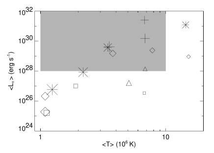
Figure 10: Mean value of the X-ray luminosity as a function of the mean value of the best fit temperature, derived from our model synthesized spectra. Crosses correspond to Mach number $M=1000$, stars to $M=300$, diamonds to $M=100$, triangles to $M=30$ and squares to $M=10$. Increasing size of each symbol corresponds to increasing value of the ambient-to-jet density contrast, $\nu=0.01$-$300$. The shaded region refers to the ($L_{\rm X}$, $T$) values consistent with observations of HH objects in general.

For a fixed value of $M$, $L_{\rm X}$ and $T$ decrease with increasing $\nu$ and, for a fixed value of $\nu$, $L_{\rm X}$ and $T$ increase with increasing $M$. From the figure it is possible to derive $M$, $\nu$ (velocity and density) of the protostellar jet to be compared with observations (in terms of $L_{\rm X}$ and best fit $T$). Predictions about fainter not yet discovered sources can also be made.

Furthermore the results derived from the variation of the initial jet density parameter, $n_{\rm j}$, discussed in Sect. 3.5, lead to the conclusion that, even with different initial density values, a protostellar jet must be less dense that the ambient medium and with high initial velocity ($1000$ km/s or more) in order to reproduce HH objects observations.

Our model predicts in all cases a significant proper motion of the X-ray source, with values which, in the case of HH 154 would be measurable with Chandra, providing a clear test of the model scenario.

As discussed by Favata et al. (2006), a 100 ks observation was performed in 2005, showing, when compared with the 2001 observation, a more complex scenario, i.e. both a moving and a stationary source were detected in HH 154, giving the source, in 2005, a “knotty” appearance. Thus, while a traveling shock (likely based on the basic physics explored in the present work) is apparently present in HH 154, the source structure is more complex.

The comparison between our model of a continuous supersonic jet through an unperturbed surrounding medium and the new Chandra data, discussed in Favata et al. (2006), shows that the model reproduces most of the physical properties observed in the X-ray emission of the protostellar jet (temperature, emission measure, etc.). At the same time, it fails to explain the complex evolving observed morphology, showing, most likely, that the jet is not continuous.

A possible scenario, which we will test in the future, is based on similar physics, but in the presence of pulsating jets (instead of the continuous jet here examined), or alternatively on interaction between the jet and an inhomogeneous ambient medium which can lead to the knotty structure observed inside the jet itself. We also plan to explore other physical mechanisms, different from the moving shock at the tip of a supersonic jet, stimulated by the above mentioned Chandra observations of HH 154, such as steady shocks formed at the mouth of a de Laval nozzle. New observations of the evolution of HH 154 will however be necessary to understand the phenomenon and to further constrain the model scenario.

The continuous jet model discussed here is a useful and necessary building block toward more complex (e.g. with a discontinuous time profile) models. The X-ray emission from a pulsed jet, for example, will still take place at the shock front, and will thus be based on the same physical effects and principles as observed in a continuous jet. Our (simpler) continuous jet model is a very useful tool to infer the right parameter values to use in future, more complex models needed to also reproduce the observed morphology: using our continuous jet model results, shown in Fig.  2 and in Fig.  10, it is possible to derive the initial jet velocity and ambient-to-jet density ratio needed for the new bullets to produce to X-ray luminosity and best fit temperature consistent with observations.

A limitation of our hydrodynamic model is the hypothesis of pressure balance between the jet and the ambient medium, in order to obtain the observed jet collimation. Most models of jet collimation suggest the presence of an organized ambient magnetic field which is known to be effective in collimating the plasma. As a follow-up of our analysis, we are developing an MHD model of protostellar jet that will allow us to relax the assumption of an initial pressure equilibrium. The comparison of the MHD model results with the X-ray observations will provide a fundamental tool to investigate the role of the magnetic field on the protostellar jet dynamics and emission.

Appendix A Synthesizing the X-ray spectra

From our 2-D numerical simulations, we synthesized the absorbed focal plane spectra to be compared with observations by using the following procedure.

As a first step, from the integration of the hydrodynamic equations  2,  3 and  4, we derive the temperature and density 2-D distributions in the computational domain.

We reconstruct the 3-D spatial distribution of these physical quantities by rotating the 2-D slabs around the symmetry axis. Then we derive the emission measure, defined as $EM=\int n_{e}n_{\rm H}dV$ (where $n_{e}$ and $n_{\rm H}$ are the electron and hydrogen densities, respectively, and $V$ is the volume of emitting plasma).

From the 3-D spatial distributions of $T$ and $EM$, we derive the distribution of emission measure $EM(T)$ for the computational domain as a whole or for part of it: we consider the temperature range $[10^{3}-10^{8}]$ K, divided into $74$ bins equispaced in $\log T$; the total $EM$ in each temperature bin is obtained summing the emission measure of all the fluid elements corresponding to the same bin.

From the $EM(T)$, using the MEKAL spectral code (Mewe et al. 1985) for optically thin plasma, we derive the number of photons in the i-th energy bin as

$$I_{i}=\frac{1}{4\pi D^{2}}\sum_{k}\int_{E_{i}}^{E_{i+1}}\frac{P(T_{k},E)EM(T_{k})}{E}dE$$ (19)

where $D$ is the distance of the object, $E_{i}$ is the energy in the i-th bin, $P(T_{k},E)$ describes the radiative losses as a function of the energy and of the temperature in the k-th bin.

To compare our model results with observations, we synthesize the focal plane spectrum, $C_{i}$, as predicted to be observed with the Chandra/ACIS-I or XMM-Newton/EPIC-pn X-ray imaging spectrometers taking into account the spectral instrumental response:

$$C_{i}=\frac{t_{exp}}{4\pi D^{2}}\sum_{k}\int_{E_{i}}^{E_{i+1}}A(E)M(i,E)\frac{P(T_{k},E)EM(T_{k})}{E}dE$$ (20)

where $t_{exp}$ is the exposure time, $A(E)$ is the effective area and $M(i,E)$ is the instrumental response.

Finally we take into account the interstellar medium absorption column density, $N_{\rm H}$ (Morrison & McCammon 1983), and we analyze the absorbed focal plane spectrum with XSPEC V11.2 in order to compare our findings with published experimental results.