A kinematic study of the Taurus-Auriga T association

Abstract

Aims. This is the first paper in a series dedicated to investigating the kinematic properties of nearby associations of young stellar objects. Here we study the Taurus-Auriga association, with the primary objective of deriving kinematic parallaxes for individual members of this low-mass star-forming region.

Methods. We took advantage of a recently published catalog of proper motions for pre-main sequence stars, which we supplemented with radial velocities from various sources found in the CDS databases. We searched for stars of the Taurus-Auriga region that share the same space velocity, using a modified convergent point method that we tested with extensive Monte Carlo simulations.

Results. Among the sample of 217 Taurus-Auriga stars with known proper motions, we identify 94 pre-main sequence stars that are probable members of the same moving group and several additional candidates whose pre-main sequence evolutionary status needs to be confirmed. We derive individual parallaxes for the 67 moving group members with known radial velocities and give tentative parallaxes for other members based on the average spatial velocity of the group. The Hertzsprung-Russell diagram for the moving group members and a discussion of their masses and ages are presented in a companion paper.

1 Introduction

To accurately determine the two main physical parameters of nearby young stellar objects (YSOs), their age and mass, we must know how far away they are. While determination of distances has been at the heart of astronomical research for many centuries, we have made surprisingly little recent progress in this respect, at least for low-luminosity objects such as the young solar-type T Tauri stars (TTSs). This contrasts with more luminous nearby stars, the targets of the very successful Hipparcos mission, for which accurate parallaxes are now available. Although Hipparcos observed a few low-luminosity pre-main sequence (PMS) stars in nearby star-forming regions (cf. Perryman et al. 1997), they were clearly a challenge for its small telescope. The situation will improve dramatically with the flight of the Gaia mission, as this satellite will measure the parallaxes and proper motions of millions of faint stars. However, Gaia’s expected launch date is 2012, so it would be useful to make some progress in determining the distances of YSOs in the meantime in order, for example, to better constrain the lifetime of their disks and the timescales of planet formation, two very timely research areas for which a precise determination of YSO ages is urgently required.

Where do we stand today as far as YSO parallaxes are concerned? The post-Hipparcos situation was discussed by Bertout et al. (1999), who provided new astrometric solutions of the Hipparcos data for groups of TTSs in various star-forming regions, thus finding average distances to some YSO groups. The new distances generally agreed well with previous estimates of the associated molecular cloud distances based, e.g., on the photometry of a few bright stars enshrouded in reflection nebulosity. For distance determinations of the Taurus star-forming region based on this method, see Racine (1968) and Elias (1978).

Although average distances provide valuable information, what we really need for constraining ages and masses by comparing observed stellar properties with evolutionary models are the distances to individual stars of the YSO associations. This is what we are attempting to do in this work, which focuses on the Taurus-Auriga T association. To do so, we use the proper motions of individual stars.

Several proper motion surveys of the Taurus-Auriga star-forming region have been performed in the past, e.g., by Jones & Herbig (1979) and Hartmann et al. (1991). More recently, Ducourant et al. (2005) published an all-sky catalog of proper motions for 1250 YSOs that provides a coherent database for kinematic studies such as the one we are now embarking on. The proper motion database for Taurus-Auriga is briefly discussed in Sect. 2.

The procedure that we use here to derive individual parallaxes is as follows. First, we identify those stars among the Taurus-Auriga confirmed or suspected YSOs that have the same spatial velocity. In other words, we look for the group of stars that defines the Taurus-Auriga T association through its common motion in the sky. While young associations are not expected to be gravitationally bound, it is well known that their members all share the same motion in space for several million years before the association dissolves and loses its identity most notably due to the tidal interactions caused by Galactic rotation and encounters with other stellar groups and interstellar clouds (see, e.g., the review by Brown 2002).

To find the likely association members, we developed our own variant of the classic convergent point method. This is described in Sect. 3, while Sect. 4 presents Monte-Carlo simulations of the moving group search that proved helpful for choosing computational parameters. We then provide lists of kinematic members in Sect. 5, where we also make use of the radial velocity information, when available, to infer parallaxes and associated error bars for individual stars. Stellar radial velocities are known only for a limited sub-sample of association members, but we can compute the average common spatial velocity of this sub-group, which in turn provides a second way of determining kinematic parallaxes for all members of the group by assuming that all stars have the same spatial velocity. These results are discussed in Sect. 6.

At that point, we should be armed with the information needed to perform a new age and mass determination for members of the moving group in the T association. This analysis and its astrophysical consequences will be presented in a companion paper (Bertout & Siess, in preparation).

2 The sample of Taurus-Auriga stellar objects

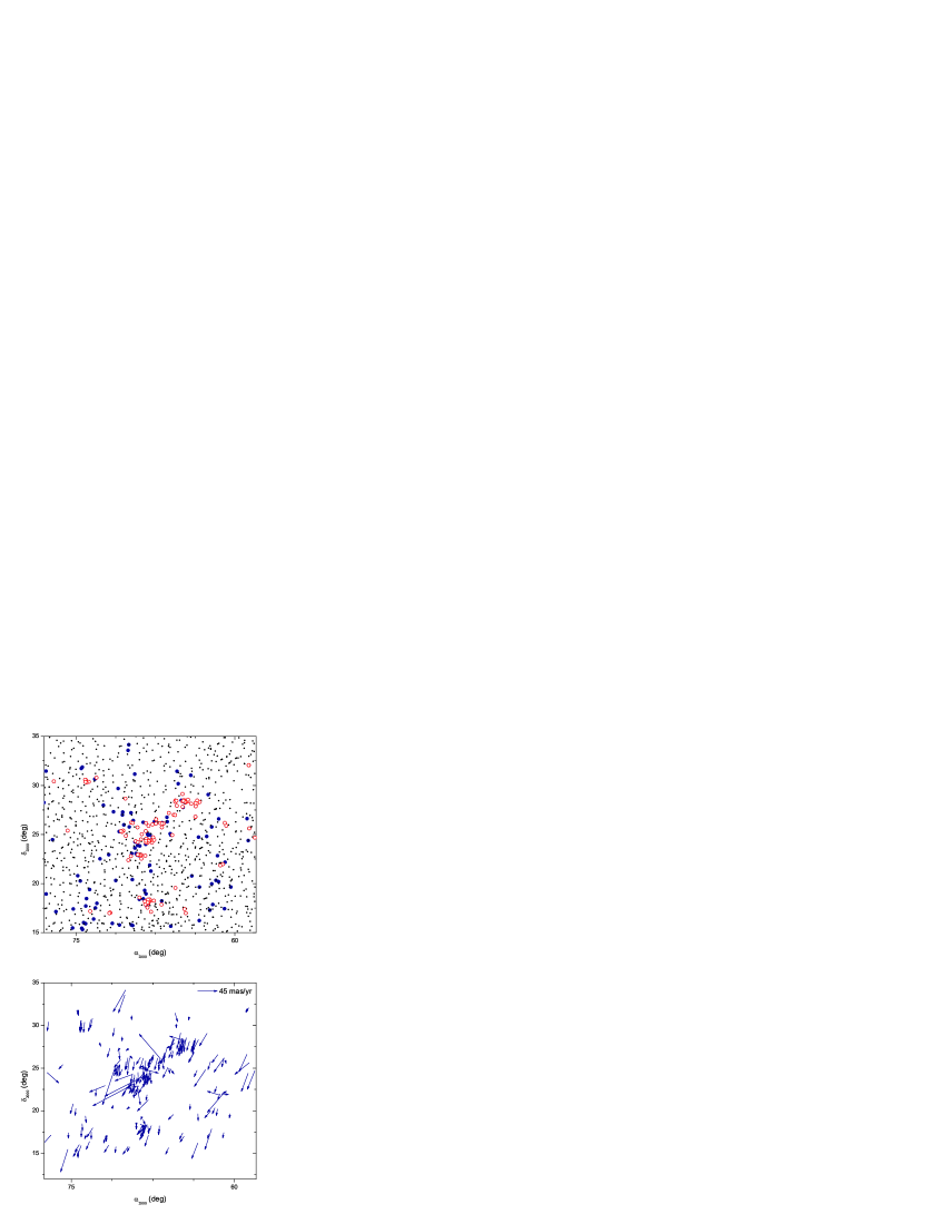
Figure 1: Upper panel: Open and filled circles indicate the positions of Taurus-Auriga stars whose proper motions are given in the Ducourant et al. (2005) catalog. The open circles denote the stars that are also included in the Herbig & Bell (1988) catalog of Orion population objects. Dots indicate the locations of stars included in the Hipparcos catalog. Lower panel: proper motion vectors of the Taurus-Auriga stars as given in the Ducourant et al. (2005) catalog.

The Ducourant et al. (2005) catalog of proper motions for PMS stars contains 217 stars that are in the general area of the Taurus-Auriga star-forming region (which roughly spans the range of coordinates $3^{h}50^{m}$ $\;\buildrel<\over{\sim}\;$$\alpha(2000)$ $\;\buildrel<\over{\sim}\;$$5^{h}10^{m}$ and $15$^∘$\;\buildrel<\over{\sim}\;$$\delta(2000)$ $\;\buildrel<\over{\sim}\;$$35$^∘).

2.1 Proper motions of Taurus PMS stars

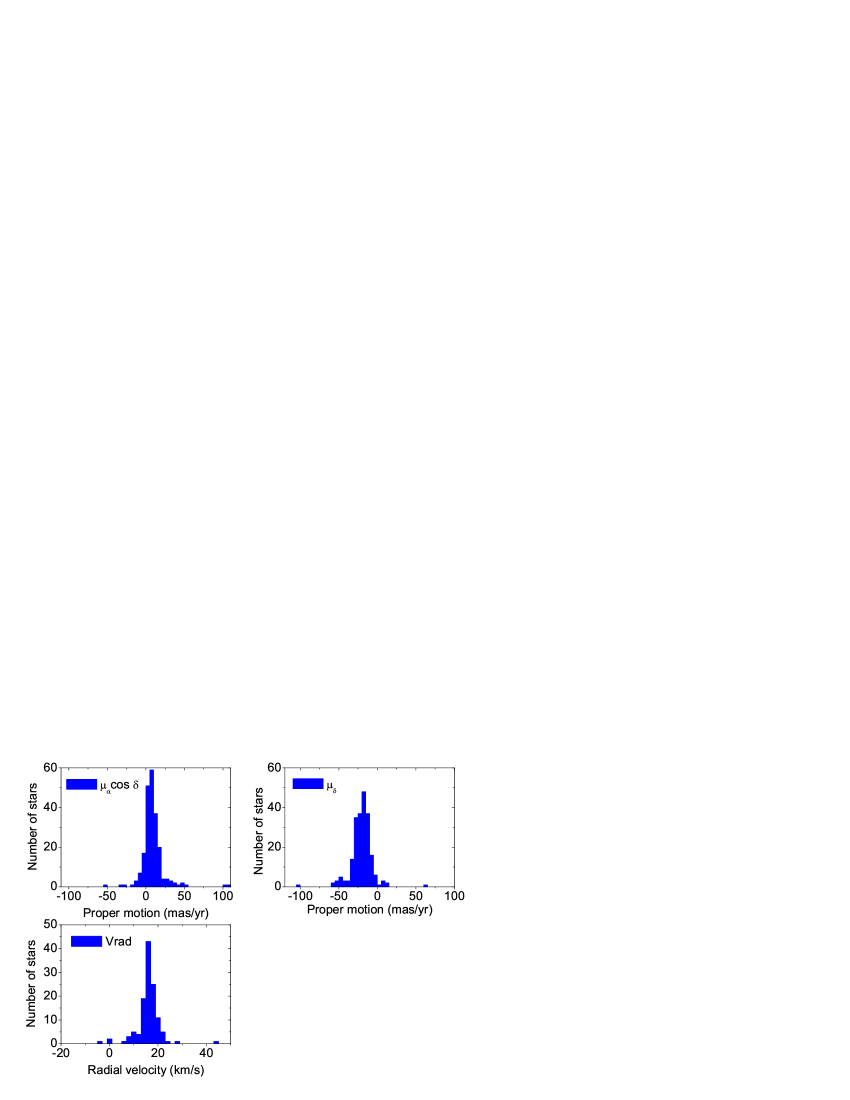
Figure 2: Proper motion and radial velocity histograms for the Taurus-Auriga stars of the Ducourant et al. (2005) catalog.

Figure 3: Proper motions and associated errors for the 217 stars considered in this investigation.

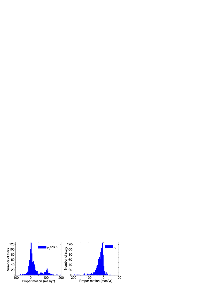
Figure 4: Proper motion histograms of the the Hipparcos stars shown in Fig 1.

Figure 5: Proper motions and associated errors for the Hipparcos stars shown in Fig 1.

The upper panel of Fig. 1 displays the location of Taurus-Auriga stars contained in the Ducourant et al. (2005) catalog. One recognizes the familiar grouping of YSOs in the vicinity of Taurus molecular cores: L1551 at approximately $\alpha(2000)=4^{h}32^{m}$ and $\delta(2000)=18$^∘. North of L1551 one finds the L1536 and L1529 groups, while in the northwest of L1529 one has the L1495 group and in the northeast the HCL2 group. The few Auriga stars present in the sample are around $\alpha(2000)=5^{h}$ and $\delta(2000)=30$^∘. Individual objects at the periphery of the molecular cloud are mainly weak emission-line TTSs discovered through their X-ray emission.

For comparison, we also show in Fig. 1 the stars observed by the Hipparcos satellite in the same region. Because of extinction, the density of Hipparcos stars strongly decreases in the vicinity of the Taurus-Auriga molecular clouds where our targets are located. As we discuss later, only a few PMS stars in the region are common to both the Hipparcos (Perryman et al. 1997) catalog and the Ducourant et al. (2005) catalog of presumably young stars.

The lower panel of Fig. 1 shows the proper motion vectors for all objects in the Ducourant et al. (2005) catalog. Although a clear convergent point for these proper motions is not readily apparent, one notices that many proper motion vectors seem to point toward the lower left-hand corner of the figure.

Figure 2 presents histograms of the proper motion components $\mu_{\alpha}\cos\delta$ and $\mu_{\delta}$, as well as a histogram of the radial velocities for those 127 objects for which we could find a published value (see below). The average values and standard deviations for the proper motions of the full sample are

$\left\{\begin{array}[]{lll}\mu_{\alpha}\cos\delta&=&8.20\pm 14.45\>\rm{mas/yr}\\ \mu_{\delta}&=&-20.82\pm 13.84\>\rm{mas/yr}\\ \end{array}\right.$

If we then consider the sub-sample of 127 stars with known radial velocities, we have

$\left\{\begin{array}[]{lll}\mu_{\alpha}\cos\delta&=&7.16\pm 8.55\>\rm{mas/yr}\\ \mu_{\delta}&=&-20.91\pm 10.31\>\rm{mas/yr}\\ v_{rad}&=&16.03\pm 6.43\>\rm{km/s},\end{array}\right.$

where we note a lower dispersion of the proper motion measurements, due in particular to the fact that radial velocities have been measured primarily in the brightest and most confirmed members of the PMS population. We come back to this point in Sect. 5.

Figure 3 displays all proper motion values and their associated uncertainties. Proper motion values cluster around the average values, albeit with considerable scatter, while a few stars have highly discrepant proper motions, often with large error bars. As discussed in Sect. 5, some of the stars included in the Ducourant et al. (2005) catalog are likely to be field stars, which explains the discrepant values. However, a majority of stars with measured radial velocities are confirmed PMS stars.

2.2 Caveats

One difficulty with the investigation envisioned here is the apparent similarity between the proper motions of field stars, as represented by the Hipparcos targets of Fig. 1, and the proper motions of our target stars. To illustrate this, we show histograms of the two proper motion components for those Hipparcos stars in Fig. 4. We also depict the proper motion data for these objects, together with their error bars, in Fig. 5.

Although the similarities with Figs. 2 and 4 are obvious, there are some differences between the proper motion distributions that become more evident when one studies the histogram shapes in more detail. We fitted these data with Gaussian curves and while it was easy to fit the proper motions of the Ducourant et al. (2005) objects with a single Gaussian, three different components were needed to fit the Hipparcos data in a satisfactory way. Actually, the three components are easily seen in Fig. 5, and Table 1 summarizes the properties of the various Gaussian curves that best fitted the data, as well as the squared coefficient of multiple correlation $R^{2}$ and the reduced $\chi^{2}$ values for the overall fits. The Ducourant et al. (2005) proper motions are marginally compatible with the proper motion values of Peak #1 of the Hipparcos proper motions but with much smaller dispersions, and the overall proper motions distributions of the two samples appear quite different. Peaks #2 and #3 correspond approximately to the proper motions of the Pleiades and Hyades clusters. We see from Fig. 1 that several stars in the Ducourant et al. (2005) catalog appear to be probable members of the Pleiades, while two stars have proper motions consistent with Hyades membership. It is therefore clear that the catalog is contaminated by non pre-main sequence stars to some extent (cf. Sect. 5).

To further quantify the differences between the proper motion distributions, we performed a Kolmogorov-Smirnov test on the two components of the proper motion for the Ducourant et al. (2005) and Hipparcos samples of stars. We found that the probability of the distributions of $\mu_{\alpha}\cos\delta$ components for both samples being drawn randomly from the same parent distribution is $8\cdot 10^{-14}$, while it is $4\cdot 10^{-7}$ for the $\mu_{\delta}$ components.

Table 1: Gaussian fits to the proper motion components of stars in the Taurus-Auriga region. The data were binned as in Figs. 2 and 4.

PM comp.	Peak #	PM	FWHM	$R^{2}$	$\chi^{2}$
		mas/yr	mas/yr
Ducourant et al. sample
$\mu_{\alpha}\cos\delta$	-	6.93 $\pm$ 0.14	12.11 $\pm$ 0.28	0.99	0.77
$\mu_{\delta}$	-	-19.29 $\pm$ 0.20	14.85 $\pm$ 0.41	0.99	0.87
Hipparcos sample
	1	0.93 $\pm$ 0.26	10.07 $\pm$ 0.67
$\mu_{\alpha}\cos\delta$	2	8.89 $\pm$ 0.95	39.38 $\pm$ 1.76	0.98	12.63
	3	103.74 $\pm$ 2.07	36.54 $\pm$ 4.17
	1	-7.77 $\pm$ 0.25	10.98 $\pm$ 0.73
$\mu_{\delta}$	2	-46.66 $\pm$ 11.34	102.12 $\pm$ 18.19	0.99	8.84
	3	-22.98 $\pm$ 1.26	31.45 $\pm$ 1.98

Figure 6: Projection on the 3 planes XY, XZ, and YZ of the spatial velocities of 127 Taurus stars with known radial velocities, assuming a common distance of 139pc. The velocity vectors originate at the stars’ coordinates in the XYZ reference frame drawn in Fig. 7. As in this figure, the spatial scales were chosen for ease of comparison with the results of this investigation.

While these differences raise the hope that the following analysis will allow us to recognize the common motion of PMS objects even in the presence of field stars, it is also clear from the above that field stars must exist that share approximately the same proper motions as the Ducourant et al. (2005) sample. Some of them could possibly contaminate the catalog, although it is meant to include – at least in principle – only PMS stars. Because we cannot kinematically distinguish between true members of the association and at least some field stars, it is crucial to scrutinize the catalog for non-PMS objects and to screen out these possible interlopers before we look for a moving group of young stars. We come back to this issue in Sect. 5.

Another worry when dealing with the kinematics of young stars in Taurus is the high degree of stellar multiplicity in that star-forming region, where the duplicity reaches about 49%, a factor 1.9 larger than for solar-type field stars (Köhler & Leinert 1998). One of the incentives cited by Ducourant et al. (2005) for preparing a proper motion catalog of PMS objects is that “dedicated work [on objects that have close companions] is necessary to derive more reliable proper motions”, and this is indeed what makes this catalog so valuable. Many binaries in Taurus are relatively wide pairs, often with large flux ratios, for which individual proper motion determinations of the components can be done. There are also a number of binaries with sub-arcsecond separations (cf. Woitas et al. 2001) that remain unresolved by Ducourant et al. (2005) and are therefore unlikely to significantly affect their results. The effect of duplicity on the catalog’s proper motions is expected to be most severe for relatively close binaries with a few arcsecond separation that were barely resolved by Ducourant et al. (2005). These systems are identified in the catalog with a mention AB that we kept in our tables. It indicates that the given proper motion is representative of the binary’s motion.

2.3 Radial velocities of Taurus PMS stars

The Herbig & Bell (1988) catalog contains all radial velocity values known prior to 1988. In order to access the more recent measurements, we searched the CDS databases using some of the data mining tools available on the CDS site. The search made use of a prototype implementation of the Unified Content Descriptors in the VizieR database.

We found radial velocity information for only 127 stars of our sample, which is quite surprising given the many investigations of the Taurus YSOs that can be found in the literature. Besides Herbig & Bell (1988), the main sources of radial velocity measurements for Taurus-Auriga stars are Joy (1949), Hartmann et al. (1986), Hartmann et al. (1987), Walter et al. (1988), Neuhäuser et al. (1997), and Wichmann et al. (2000). While we might have missed some data that are not included in the CDS databases or are not known to us otherwise, it is also obvious that investigations of Taurus-Auriga have often focused on the same relatively bright stars in the region, and no systematic, high-precision radial velocity survey has been performed to date in spite of the availability of efficient spectrographs on medium-sized telescopes.

2.4 Galactic velocities of the Ducourant et al. (2005) sample

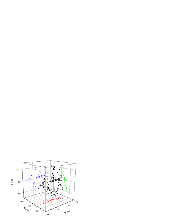
Figure 7: The 3D spatial distribution of the 127 Taurus stars with known radial velocities, assuming a common distance of 139 pc, in a cube with sides equal to 60 pc. The XYZ reference frame is defined in the text; the Sun is located at its origin. The ball-like symbols represent individual stars whose projections on the 3 planes are shown as small squares with different colors.

We now compute the Galactic positions and velocities of the 127 stars for which we know radial velocities, using the method delineated in Johnson & Soderblom (1987). The Galactic positions are defined on an $XYZ$-grid with the origin at the Sun. There, $X$ points to the Galactic center, $Y$ points in the direction of Galactic rotation, and $Z$ points to the Galactic North pole. The projection of the Galactic velocity on the same grid defines the components $U$, $V$, and $W$.

We plotted the projections of the Galactic velocities onto the three planes $XY$, $XZ$, and $YZ$ in Fig. 6, mainly for the purpose of comparison with the results obtained in the following sections. Using the direction of the equatorial coordinate system south-north axis indicated above, one can check that the directions of velocity projections in the $YZ$-plane follow the directions of the proper motion vectors of Fig. 1, as expected. Although there is an obvious scatter in the velocity directions, it appears from these projections that a number of stars may have similar space motions, thus providing an incentive for the following investigation.

Figure 7 is a 3D cube with sides equal to 60 pc showing the Galactic positions of the Taurus stars when, following Bertout et al. (1999), we assume an average distance of 139 pc for the Taurus complex. With this average distance, the stars populate an $XZ$-plane at $X\approx-132$ pc, and one recognizes the T Tauri stellar groupings in this plane. Note that the south-north axis of the equatorial coordinate system runs approximately parallel to the direction of the diagonal from $Z=-70$, $Y=-20$ to $Z=-10$, $Y=40$. The size of the 3D cube was chosen for comparison with the results of Sect. 5.

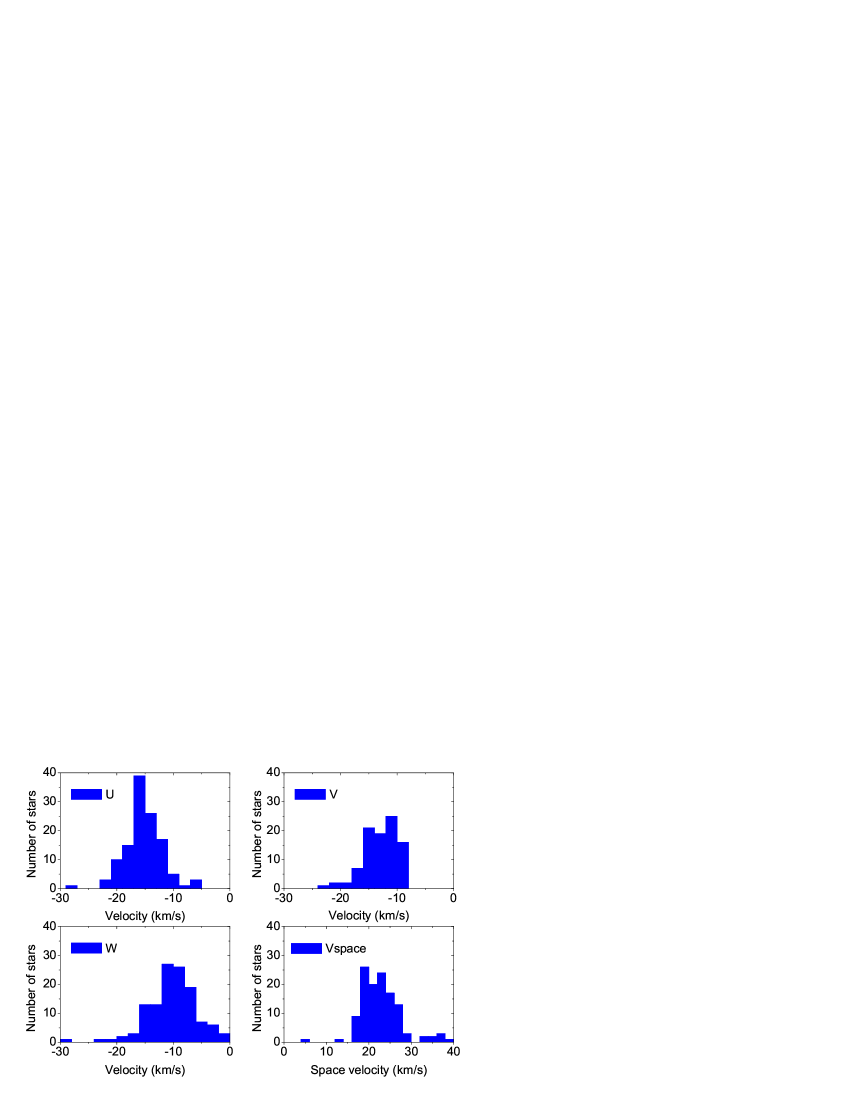
Figure 8: Histograms of the U, V, W Galactic velocity components, as well as the magnitudes of the spatial velocities for 127 Taurus stars with known radial velocity, assuming a common distance of 139pc.

Finally, we have plotted histograms of the $U$, $V$, $W$, and $V_{rad}$ values in Fig. 8. Their respective average and standard deviation values are

$\left\{\begin{array}[]{lll}U&=&-15.37\pm 6.00\>\rm{km/s}\\ V&=&-11.74\pm 6.50\>\rm{km/s}\\ W&=&-9.89\pm 4.94\>\rm{km/s}\\ V_{space}&=&23.20\pm 5.98\>\rm{km/s}.\end{array}\right.$

3 Method of analysis

We have developed our own variant of the well-known convergent point method for finding members of moving groups that share the same space motion. The original method goes back to Charlier (1916) and was further developed by several workers, including Brown (1950), Jones (1971), and more recently by de Bruijne (1999), who adapted it so as to take full advantage of the Hipparcos data. We review briefly the method before outlining the variant we developed to deal with the problem at hand.

3.1 The classic convergent point method

The convergent point method is based on the fact that the proper-motion vectors of a group of stars moving with the same motion in space appear to an observer to converge to a specific point of the sky plane, called the convergent point (CP hereafter).

The two components of the proper motion vector $\@vec{\mu}$ in the equatorial coordinate system, $\mu_{\alpha}\cos\delta$ and $\mu_{\delta}$, define the tangential velocity vector $\@vec{v_{tan}}$ through the relation

$$\@vec{v_{tan}}\equiv\frac{A\>\@vec{\mu}}{\pi}$$ (1)

where $\pi$ is the parallax in milliarcseconds (mas) and where $A=4.74047$ km yr/s, the ratio of one astronomical unit in km to the number of seconds in one Julian year, is the constant needed for adjusting the units on both sides of the equation.

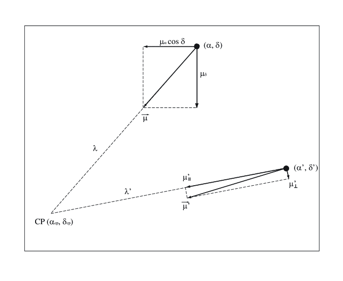
Figure 9: Schematic representation of the various proper motion components used in this analysis. See text for details.

If we denote the modulus of the space velocity vector by $\left|\;\@vec{v}\;\right|$ and, for the time being, neglect measurement errors and a possible internal cluster velocity dispersion, we have

$$\left|\;\@vec{\mu}\;\right|=\frac{\pi\left|\;\@vec{v}\;\right|\sin\lambda}{A}$$ (2)

where $\lambda$ is the angular distance between the position ($\alpha,\delta$) of a given star in the moving group and the position ($\alpha_{CP},\delta_{CP}$) of the convergent point (see the schematic representation in Fig. 9). Spherical trigonometry tells us that

$$\cos\lambda=\sin\delta\sin\delta_{CP}+\cos\delta\cos\delta_{CP}\cos(\alpha_{CP}-\alpha).$$ (3)

If we now change coordinates (see Fig. 9) and project the proper motion onto the axis joining the star to the CP, on one hand (component $\mu_{\parallel}$), and onto the perpendicular direction, on the other (component $\mu_{\perp}$), the proper motion components in both systems are related by

$$\left\{\begin{array}[]{l}\mu_{\parallel}=\sin\theta\>\mu_{\alpha}\cos\delta+\cos\theta\>\mu_{\delta}\\ \mu_{\perp}=-\cos\theta\>\mu_{\alpha}\cos\delta+\sin\theta\>\mu_{\delta}.\end{array}\right.$$ (4)

with

$$\tan\theta=\frac{\sin(\alpha_{CP}-\alpha)}{\cos\delta\tan\delta_{CP}-\sin\delta\cos(\alpha_{CP}-\alpha)}.$$ (5)

If the proper motion vector is directed exactly toward the CP, then we also have

$$\left\{\begin{array}[]{l}\mu_{\parallel}=\frac{\pi v\sin\lambda}{A}=\left|\;\@vec{\mu}\;\right|\\ \mu_{\perp}=0.\end{array}\right.$$ (6)

In general, the measurement errors $\sigma_{\perp}$ and velocity dispersion within the moving group $\sigma_{int}$ (expressed in mas/yr) conspire to make $\mu_{\perp}$ different from zero, but the expectation value of this quantity for any star belonging to a moving group is zero. If one assumes, following de Bruijne (1999), that the error-weighted value of $\mu_{\perp}$, defined as

$$t_{\perp}\equiv\frac{\mu_{\perp}}{\sigma_{tot}}$$ (7)

where

$$\sigma_{tot}\equiv\sqrt{\sigma_{\perp}^{2}+\sigma_{int}^{2}},$$ (8)

is distributed normally with zero mean and unit variance for all stars in the moving group, then the probability distribution for a given combination of $\mu_{\perp}$ and $\sigma_{tot}$ to occur is

$$p_{ind}=\frac{1}{\sqrt{2\pi}}\exp(-\frac{t_{\perp}^{2}}{2}).$$ (9)

The CP method for finding a moving group within a cluster of $N$ stellar candidates, as implemented by Jones (1971), goes through the following steps (see also de Bruijne 1999).

1. First define a grid $(i,j)$ in the plane of the sky $(\alpha,\delta)$, where $i$ and $j$ vary from 1 to $N_{grid}$. The grid defines candidate CP positions.

2. At each grid point $(i,j)$, use Eq. 7 to compute the expression

   $$X^{2}=\sum_{k=1}^{N}(t_{\perp}^{2})_{k}$$ (10)

   where the index $k$ runs over all stars. With $t_{\perp}^{2}$ distributed normally, $X^{2}$ is distributed as $\chi^{2}$ with $N-2$ degrees of freedom. Minimizing $X^{2}$ is equivalent to maximizing the likelihood that the computed set of $t_{\perp}$ occurs, and the most likely CP is therefore the grid point with the lowest $X^{2}$ value.

3. However, it could still occur that the lowest value of $X^{2}$ is due to chance rather than to a good fit between observations and the model. To evaluate this possibility, one calculates the probability $p_{min}$ for $X^{2}$ to be higher than its computed value by chance even if the derived CP is the correct one. This probability is given by the incomplete gamma function

   $$p_{min}=\frac{1}{\Gamma[\frac{1}{2}(N-2)]}\int_{X^{2}}^{\infty}x^{\frac{1}{2}(N-2)-1}\,\exp(-x)\,dx.$$ (11)

4. If $p_{min}$ is too low, then one rejects the star with the highest $\left|\,t_{\perp}\,\right|$, corrects the number of stars and goes back to step 2.

5. One then continues until $p_{min}$ has reached an acceptable value (to be discussed later). When this is done, all remaining stars are defined as bona fide group members and the most likely CP candidate in the last iteration is defined as the convergent point of the group.

As noted by de Bruijne (1999), the basic equations of the method (Eqs. 2 and 6) remain valid if the stars belonging to the association are in a state of uniform expansion. In that case, however, using the proper motion information to determine the CP as we do here implies that the derived velocity $\@vec{v}$ is the sum of the actual space motion and the reflex motion of the expansion, and these two motions cannot be disentangled.

Another caveat with the above method is its bias towards low $t_{\perp}$, which is unavoidable since on principle the CP search favors low values of this parameter. However, not all stars with low $t_{\perp}$ are necessarily moving group members; both stars with intrinsically small proper motions and stars located at large distances have a low $t_{\perp}$.

It is therefore customary to eliminate stars with insignificant proper motions prior to doing the analysis, because such objects would not be rejected in the CP search. The criterion for rejection (de Bruijne 1999) is

$$t=\frac{\mu}{\sigma_{\mu}}=\frac{\sqrt{\mu_{\alpha}^{2}\cos^{2}\delta+\mu_{\delta}^{2}}}{\sqrt{\sigma^{2}_{\mu_{\alpha\cos\theta}}+\sigma^{2}_{\mu_{\delta}}}}\leq t_{min}$$ (12)

where $t_{min}$ depends on the quality of the data (see below). While this preliminary step eliminates a number of non-group members, it does nothing to correct the bias toward selecting the most distant stars in the group as members.

3.2 Modified CP method

The main difficulty that we encountered while using this method of finding a moving group of stars in Taurus is due to a combination of two properties of this region. First, the Taurus-Auriga star-forming region spans a large volume, but the YSOs are bunched in small groups with vast spaces devoid of stars between them rather than being distributed more evenly on the plane of the sky, as, e.g., older open clusters are. This specific morphology complicates the search for the CP, since the most likely CP position wanders in the plane of the sky depending on the groups of stars that dominate $X^{2}$ during a given iteration. As a consequence, a large number of possible group members may well be eliminated before $p_{min}$ reaches a reasonable value. Moreover, the remaining stars are the most distant ones, as explained above.

Second, there is a velocity dispersion between the different parts of the Taurus star-forming region of several km/s, which was first noted by Jones & Herbig (1979) and confirmed by subsequent investigators. Although this velocity dispersion is taken explicitly into account in the CP method, it reduces both the computed individual probabilities $p_{ind}$ (Eq. 9) of stars being members of a moving group and the likelihood that the computed set of $t_{\perp}$ occurs, thus making it more difficult to reach a high $p_{min}$. Extensive Monte-Carlo simulations (cf. Sect. 4), which assumed a group of stars with the same positions as our sample and various sets of parameters, indeed confirmed that both the size of the recovered moving group and the probability of recovering the correct average distance for that moving group decreases with increasing internal velocity dispersion.

One possibility for considering the specificities of our sample would be to use the CP search procedure as described above while lowering the requirement on $p_{min}$ to a value in the range $10^{-1}$. However, we felt uncomfortable with settling for low $p_{min}$ values that do not confirm the reality of the derived moving group. For comparison, de Bruijne (1999) chose $p_{min}$ equal to 0.954 in his study of moving groups, also on the basis of Monte-Carlo simulations.

Instead, we devised a modification of the CP method that helped us to find the moving group while giving very low probabilities that the solution was due to chance. The idea is to provide some initial guidance to the code by first guessing the CP position (exploiting the available radial velocity data) and eliminating those stars with the most obviously discrepant proper motions before proceeding with the classic CP search as described above.

For the initial guess of the CP position, we used the sub-sample of stars with known radial velocities $v_{rad}$ and the average, post-Hipparcos Taurus-Auriga parallax value derived by Bertout et al. (1999). Starting from Eq. 1, which defines the two tangential components $v_{\alpha}$ and $v_{\delta}$, we converted the velocity components in the equatorial system to a rectangular coordinate system $(x,y,z)$ in which $x$ points towards the vernal equinox, $y$ is directed towards the point on the equator with $\alpha=\pi/2$, and $z$ points towards the Northern equatorial pole. The conversion is done by the following transformation

$$\left(\begin{array}[]{c}v_{x}\\ v_{y}\\ v_{z}\end{array}\right)=\left(\begin{array}[]{ccc}-\sin\alpha&-\sin\delta\,\cos\alpha&\cos\delta\;\cos\alpha\\ \cos\alpha&-\sin\delta\;\sin\alpha&\cos\delta\;\sin\alpha\\ 0&\cos\delta&\sin\delta\end{array}\right)\left(\begin{array}[]{c}v_{\alpha}\\ v_{\delta}\\ v_{rad}\end{array}\right).$$ (13)

An approximate CP location is then given by

$$\left\{\begin{array}[]{lll}\alpha_{CP}&=&\arctan\left(\frac{\overline{\textstyle v_{y}}}{\overline{\textstyle v_{x}}}\right)\\ &&\\ \delta_{CP}&=&\arctan\left(\frac{\overline{\textstyle v_{z}}}{\left(\overline{\textstyle v_{x}}^{2}+\overline{\textstyle v_{y}}^{2}\right)^{1/2}}\right)\end{array}\right.$$ (14)

where $\overline{v_{x}}$, $\overline{v_{y}}$, and $\overline{v_{z}}$ are the averages of the velocity components over the sample of stars with known radial velocities.

Once this first guess of the CP coordinates was completed, we computed the individual probability of each star being part of a moving group converging to this point by using Eq. 9 and eliminated those objects for which $p_{ind}$ was lower than a preset value.

We then proceeded with the usual CP method as described above. Monte-Carlo simulations with various sets of parameters reported in Sect. 4 show that the convergence to a highly probable solution is very quick after the initial elimination of discrepant stars. Note also that the overall probability that the group is not due to chance is generally very close to one, and much higher when we perform such an initial screening than when using the usual CP method, which confirms that this simple procedure eliminates those interlopers whose proper motions are not compatible with the derived CP. Conversely, and this is the main drawback of the modified method, more bona fide group members are usually eliminated than when using the usual CP method, depending on the choice of computational parameters.

We should not expect this modified CP search method to produce results that are different from the classic method – both methods rely in essence on the same procedure – unless the initial CP guess biases the final result. This can be checked because the second step of the search allows for an iteration of the CP coordinates. In the Monte-Carlo simulations discussed in Sect. 4, the final CP coordinates are usually close to the coordinates of the initial guess, thus confirming the lack of appreciable bias. We emphasize that the only advantage to this search strategy over the classic one for the stellar group under investigation is that it often leads to a converged solution, whereas the classic method fails to converge due to the specific properties of Taurus-Auriga discussed above.

3.3 Parallax computations

Once we have defined a moving group, we can derive the kinematic parallaxes $\pi_{Vrad}$ of individual group members and their uncertainties, if we know their radial velocities $V_{rad}$. We have

$$\pi_{Vrad}=\frac{A\mu_{\parallel}}{V_{rad}\tan\lambda}$$ (15)

where $\lambda$ is given by Eq. 3. The error on $\lambda$ is computed as in de Bruijne (1999), and standard error propagation techniques lead to a determination of the uncertainty on $\pi$.

In order to estimate approximate individual parallaxes of group members with unknown radial velocities, we derive the average spatial velocity $V_{group}$ from the Galactic velocity components of the stars with known radial velocities and use the relationship

$$\pi_{Vgroup}=\frac{A\mu_{\parallel}}{V_{group}\sin\lambda}.$$ (16)

Again, one can derive the uncertainty on $\pi$ from the uncertainty on the group velocity, $\mu_{\parallel}$ and $\lambda$. A comparison of both parallax estimates is made in the section describing the results for Taurus-Auriga (Sect. 5).

This ends the general description of the method used to find the moving group members and their individual parallaxes. In the following section, we present the extensive Monte-Carlo simulations that were used to test our alternate CP method and compare it to the classic one.

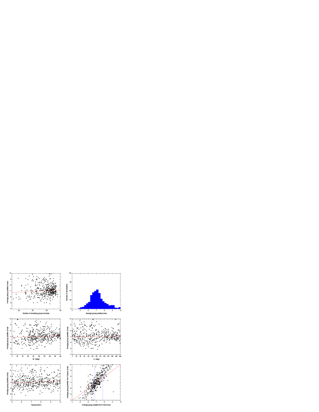
Figure 10: Results of the classic CP search for Simulation 1, the parameters of which are given in Table 2. Upper left panel: relationship between the average group parallax and the number of group members identified by the CP search for each realization. Upper right panel: histogram of recovered parallaxes. Middle left panel: average parallax as a function of the angle $\Theta$. Middle right panel: average group parallax as a function of the angle $\Phi$. Lower left panel: average parallax as a function of the initial group velocity. Lower right panel: comparison of the recovered parallaxes using either the observed radial velocities of individual stars or the average space velocity of the group, as discussed in the text. Linear, error-weighted fits to the data points are also shown in each panel, except for the lower right one, where for the purpose of comparison we have drawn a straight line indicating perfectly correlated parallaxes. The two vertical lines at $\pi=6.3$ and $\pi=7.8$ indicate the $\pm 1\sigma$ range of parallaxes assigned to synthetic stars in the simulations.

Figure 11: Results of the variant CP search for Simulation 5. See the caption of Fig. 10 for details.

4 Monte-Carlo simulations of the moving group search

Monte-Carlo simulations are often useful for exploring the role of the various parameters in numerical methods such as the CP search. They are also crucial for gaining confidence in the derived results.

J. de Bruijne (1999) performed extensive simulations that convincingly demonstrate the ability of the CP method to find and eliminate interlopers, i.e., field stars that are seen projected against the stellar group but are not members of the moving group. The method also eliminates stars from the moving group that are actual members, and the computation parameters are chosen so as to find the largest number of likely group members.

In our simulations we focused mainly on how the classic CP method and its alternative deal with the large internal velocity dispersion found in our stellar sample, as well as with the relatively large uncertainties in the measured proper motions. These two aspects were not discussed by de Bruijne (1999) since he was dealing with groups having low internal velocity dispersion and using accurate Hipparcos proper motions. We also investigated how interlopers affect our results.

4.1 Monte-Carlo simulation set-up

In the following, we compare results obtained using the same data sets by the classic CP method, on one hand, and by its variant with an initial guess of the CP coordinates, on the other.

We constructed our synthetic groups of stars in the same way as de Bruijne (1999). The total number of stars that we used in these simulations was 117, corresponding to the sample common to both the Ducourant et al. (2005) and Herbig & Bell (1988) catalogs. This choice of sample is justified in Sect. 5. Each synthetic star had the same equatorial coordinates as one of our program stars. For each realization, we randomly chose a group spatial velocity that is shared by all members of the data set. This was done by randomly drawing the velocity modulus in a given interval (typically between 5 and 10 km/s), as well as the two angles $\Theta$ and $\Phi$ defining its direction in the $(X,Y,Z)$ coordinate system. We note in passing that the approximate values of these parameters for the Taurus-Auriga group discussed in Sect. 5 are $V_{group}=7.3$ km/s, $\Theta=116^{\circ}$, and $\Phi=171^{\circ}$. We have neglected in this derivation the small correction accounting for the difference between the Galactic rotation values for the Sun and the Taurus region.

In some simulations, we injected a certain percentage of field stars (between 3 and 10% – see discussion in the following section) in order to test the response of the code to their presence. This was done randomly and the proper motion values were assigned by randomly drawing a star from the sample of Hipparcos stars described in Sect. 2. Since Hipparcos measurement uncertainties are lower than in our sample, we added measurement errors to these data using the procedure described below for moving group members. If the coordinates of the simulated interloper corresponded to a catalog star with known radial velocity, we assigned the observed value of the radial velocity and its uncertainty to the interloper.

Otherwise, stars were considered to be members of the moving group and we thus computed the expected values of the Galactic velocity components from the assumptions described above. We then added a randomly drawn velocity dispersion to each velocity component. These internal motion components were normally distributed with width $\sigma_{int}$. In many simulations, we used $\sigma_{int}\approx 6$ km/s, which is representative of the velocity dispersion of our stellar sample as found in proper motion surveys. The Taurus star-forming region is made up of subgroups of stars, the members of which are sometimes separated by only a few tenths of a parsec in projection. In these subgroups, the velocity dispersion of individual stars is much smaller than the dispersion between the velocities of various subgroups (cf. Jones & Herbig 1979). In the simulations, we therefore assumed that velocities of stars closer than 1 pc in projection were the same except for measurement errors.

Once the velocity dispersion was added to the Galactic velocity components, the values $(U,V,W)$ were corrected for the solar motion, using $(U,V,W)_{\odot}=(9.88,14.19,7.76)$ km/s (Mignard 2000). The stellar parallax was then drawn from a normal distribution centered on the average parallax of Taurus with width equal to the standard error computed by Bertout et al. (1999): $\pi_{Taurus}=7.31\pm 0.49$ mas.

From there, proper motions and radial velocities were computed and measurement errors added to the results. In the simulations reported here, we drew random errors from a normal distribution with width equal to the average uncertainties of the observed proper motions and radial velocities. In other simulations not illustrated here, we used the observational uncertainties given in the Ducourant et al. (2005) catalog for the members of the moving group. The simulation results were similar to those reported here. Note that we assigned a radial velocity value only to those objects that simulated stars with known radial velocity in our data set. Finally, we added the Galactic rotation using the first-order formulae and the same Oort constants as de Bruijne (1999).

After constructing such a synthetic data set, we ran the CP search and recorded various simulation parameters $(v_{group},\Theta,\Phi)$ and some of the results, notably the number of group members recovered by the search and the average group parallax, which can be directly compared to the known input parameters.

4.2 Results

Table 2: Parameters and main results of Monte-Carlo simulations

Simulation	1	2	3	4	5	6	7
Figure	10	-	-	11	-	-	-
Parameters
$\sigma_{dis}$	6	6	6	6	6	6	3
$\sigma_{PM}$	5	5	5	5	5	5	2
$N_{intl}/N_{total}$	0	0	0	0	0.03	0.1	0
$1-p_{min}$	$10^{-1}$	$10^{-5}$	$10^{-5}$	$10^{-10}$	$10^{-10}$	$10^{-10}$	$10^{-10}$
$p_{ind}$	-	0.6	0.7	0.8	0.8	0.8	0.7
Results
$p_{\pi}$	0.32	0.44	0.44	0.51	0.49	0.48	0.64
$f$	0.18	$<0.02$	$<0.02$	$<0.02$	$<0.02$	$<0.02$	$<0.01$
$\bar{N}/N_{total}$	0.84	0.84	0.81	0.75	0.73	0.69	0.91

We constructed 500 such data-set realizations when running one Monte-Carlo simulation for a given set of CP-search parameters. Some results are reported below.

Table 2 gives the main parameters of the simulation, i.e., the internal velocity dispersion $\sigma_{dis}$ in km/s, the average uncertainty of proper motions measurements $\sigma_{PM}$ in mas/yr, the requested minimum probability that the group is not due to chance, as well as the minimum individual probability of a star being a group member (see Sect. 3). When the classic CP method is used, this parameter is not needed, and the entry is marked as $-$. The simulation results, also summarized in the table, are the probability $p_{\pi}$ of recovering the parallax within the assumed error bars for a given set of simulations, the percentage $f$ of cases for which the moving group was not detected, and the average number of recovered group members in percentage $\bar{N}/N_{total}$.

The main results are illustrated by two figures. Figure 10 shows results of the classic CP search for Simulation 1, and Fig. 11 shows a set of results obtained using the alternate CP search method, with parameters close to the ones we chose for the actual computations. These two figures have six panels each, and their contents are described in the caption of Fig. 10.

Simulation 1 implements the classic CP method for group parameters similar to those of our data set. Table 2 shows that the probability of recovering the true parallax of the moving group is only 0.32, and the failure rate $f$ of detecting the moving group is as high as 18%, whereas 84% of the moving group members are recovered when using this method.

Simulations 2 to 7 implement the modified CP method discussed in Sect. 3. Results are given for three different values of the threshold value for the individual probabilities $p_{ind}$ of a star being a group member, for two values of the $(\sigma_{disp},\sigma_{PM})$ parameter couple, and for three values of $N_{intl}/N_{total}$, the fraction of interlopers among the sample of stars. The results obtained with $p_{ind}=0.6$ (Simulation 2) roughly correspond to those of the classic CP method in the sense that 84% of the group members are recovered, but the failure rate for finding a moving group is much lower ($<$ 2%), and the probability of recovering the right average parallax is 44%.

As expected, the number of recovered group members decreases with increasing $p_{ind}$, while the probability of recovering the true parallax reaches about 0.5 for $p_{ind}\approx 0.8$.

We should note here that the total number of stars in the sample has little influence on the results, as long as it is sufficiently large for this statistical search method to be meaningful. In addition to the simulations reported here, which used 117 stars, we performed simulations for the total sample of 217 stars. Results with this larger group differed little from those reported in this section, although the probabilities of recovering the right average parallax value were higher by a few %.

One also notes that the probability of detecting the moving group with this method is always very high once $p_{ind}>0.6$. The method appears tolerant of an interloper fraction up to 10% (Simulations 5 and 6), which barely affects the results. In all cases we investigated, about half of the interlopers were rejected as non-members of the moving group, while the second half remained undetected.

The last simulation considers lower values of the internal velocity dispersion and proper motion measurement errors, and confirmed that the CP search is much more accurate when high quality data are available and the internal velocity dispersion is small. We should nevertheless emphasize here that there is no need to use this alternate CP search method when the internal velocity dispersion and proper motion measurement uncertainties are as low as in this last simulation; the classic CP search method works very well in such cases.

There is no apparent correlation between the average parallax derived from the CP search and the group velocity for the range of velocities (5 to 10 km/s) that we investigated here. For these low group velocities, there is a correlation between the derived parallax and the angles $\Theta$ and $\Phi$, in the sense that the dispersion of recovered parallaxes is smallest for in range of angles for which the contrast between reflex solar motion and group motion is highest.

Table 3: Taurus-Auriga stars with insignificant proper motions

Star	HBC
NTTS 040012+2545 AB	357
NTTS 040142+2150SW	360
NTTS 040142+2150NE	361
DH Tau	38
V710 Tau AB	51
CoKu HP Tau G3	414
CoKu Tau-Aur Star 4	421
DQ Tau	72
Haro 6-37 AB	73
StHA 34	425
V836 Tau	429

Results of the alternate CP search method are sensitive to the threshold probability $p_{ind}$, which must be carefully chosen to achieve the best possible compromise between $p_{min}$ and the recovered number of group members. Extensive tests suggest an optimal threshold value in the range $0.7-0.8$ for our data set.

Parallaxes are computed in two ways. First, we use the radial velocity information to compute parallaxes for the subset of stars for which this quantity is known. Once this is done, we compute the average group velocity for this subset and then assume that it is the group velocity of all stars in the moving group. Approximate parallaxes can then be computed for all stars in the moving group. We compared the average moving group parallaxes obtained by these two methods (see Figs. 10 and 11), and conclude that they give similar results within the computed uncertainties when the recovered average parallaxes are in the correct range (delimited by two vertical lines in the figures). The general bias of the CP method toward lower parallaxes that we discussed earlier is apparent in these figures.

4.3 Conclusion

We have presented an alternate CP search method suitable for dispersed stellar groups with large internal velocity dispersions. For such groups, the classic CP method often fails to converge or to give realistic results. The alternate method is much less computationally intensive and nearly always converges when a moving group is present, provided the fraction of interlopers is not too large. However, it tends to eliminate more actual group members than the classic method does. Its use should therefore be limited to cases where the classic method is expected to fail.

Figure 12: Projection on the 3 planes XY, XZ, and YZ of the spatial velocities for the Taurus moving group members with known radial velocities. The velocity vectors originate at the stars’ coordinates in the XYZ reference frame.

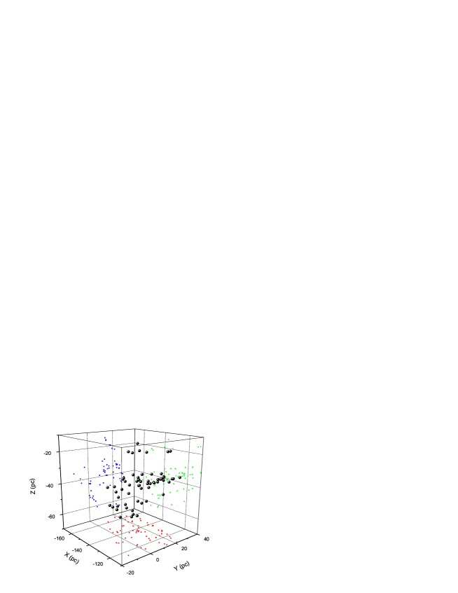
Figure 13: 3D spatial distribution of the Taurus moving group members with known radial velocities. The ball-like symbols represent individual stars whose projections on the 3 planes are shown as small squares with different colors. Table 5 gives the Galactic coordinates and velocities of individual objects.

5 Application to Taurus-Auriga

As discussed in Sect. 2, we should expect that an undefined, but probably significant, number of field stars are not distinguishable, as far as their kinematics are concerned, from the PMS stars that we are interested in. A consequence, demonstrated by the simulations reported in Sect. 4, is that up to about 50% of those interlopers may remain undetected even though a moving group has been identified and hence may pollute the results. The best way to proceed is thus to preemptively screen out the main sequence stars that may possibly be present in our sample before searching for a moving group among the young stellar population. A critical discussion of the PMS status of the stars included in the Ducourant et al. (2005) catalog is thus in order. This is done in the next subsection, where we divide the Taurus-Auriga sample into two subsets, one for stars that are clearly of PMS nature, and the other for stars in a more uncertain evolutionary state. We then discuss the values chosen for the parameters that enter the computation, present the results of the kinematic analysis for both subsets of stars, and give the list of moving group members with their individual parallaxes.

5.1 Refining the PMS star sample

In their proper motion catalog for PMS stars, Ducourant et al. (2005) include a flag indicating the “classification as given by CDS or found in the literature : T=T Tauri (CTT or WTT), A = HAeBe, Y = YSO, W = WTT, P = PMS, X = X-ray active source (Li 2000, table 2), O = Post T Tauri, L = Emission Line from HBC catalogue, Tc = T Tauri candidate, Wc = WTTs candidate. Ac = HAeBe candidate, Yc = YSOs candidate, Pc = PMS candidate”. It is already apparent from this list that the catalog might well be contaminated by main sequence stars, since many X-ray active main sequence stars exist and also since the evolutionary status of the various “candidates” above is unclear. A closer look at the list of catalogued objects unveils an even more serious problem because most X-ray sources that are detected in the general direction of Taurus are noted as PMS objects, although there is a large body of evidence suggesting that they are, at least in part, active main-sequence stars (e.g., Gomez et al. 1992; Briceno et al. 1997; Neuhäuser et al. 1997; Wichmann et al. 2000). Depending on what fraction of the stars detected through their X-ray emission are truly PMS, there could be a sizable number (perhaps up to 30%) of field stars in the sample of “PMS” stars discussed in Sect. 2.

We devised the following strategy to circumvent the problem created by the presence of potential field stars in our sample.

1. We chose a sub-sample of highly probable PMS objects by restricting the Ducourant et al. (2005) sample to stars contained in the Herbig & Bell (1988) catalog of confirmed Orion population members and ran the CP search for that group of 117 objects, thus looking for a core Taurus-Auriga moving group.

2. Using the derived CP coordinates, we computed the probability of each star in the full sample of 217 stars being a member of the core moving group and defined as possible additional members those stars whose probability of membership was sufficiently high.

3. We then verified, from a thorough literature search, the PMS status of stars belonging to this extended moving group in order to eliminate the possibly remaining interlopers.

The details of the process are given below.

5.2 Choice of computation parameters

There are five such parameters: the number $N_{grid}$ of trial grid points for the CP search, the value $t_{min}$ that defines the magnitude of insignificant proper motions (see Eq. 12), the velocity dispersion $\sigma_{int}$ that determines the basic quantity $t_{\perp}$ (Eq. 7), the threshold probability $p_{min}$ (Eq. 11) for deciding that the moving group is not a chance occurrence, and the threshold probability $p_{ind}$ (Eq. 9) of individual stars being considered as possible moving group members in the initial screening described above.

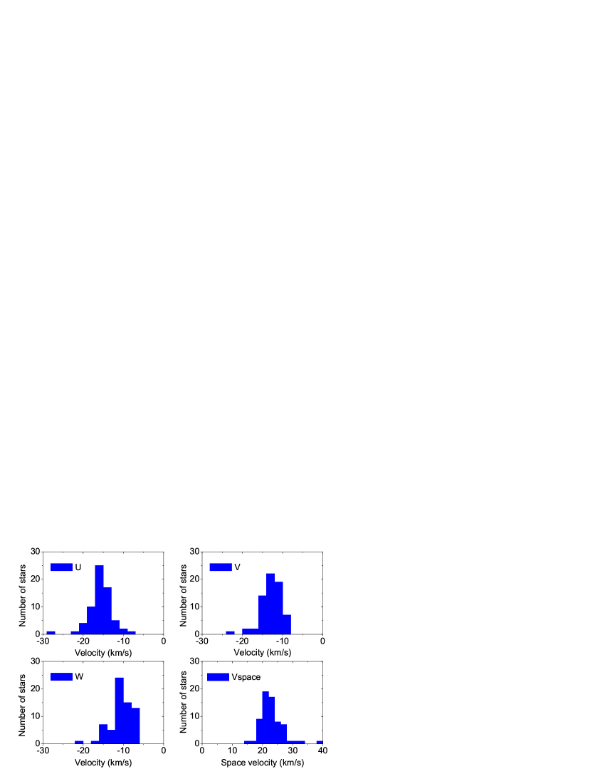
Figure 14: Histograms of the U, V, W galactic velocity components and spatial velocity for members of the Taurus moving group with known radial velocities.

Table 4: Parallaxes (in mas) and distances (in pc) of 58 moving group stars with known radial velocities.

Star	HBC	$\pi_{Vrad}\pm\sigma_{\pi}$	$d_{Vrad}\pm\sigma_{d}$
NTTS 035120+3154SW	352	3.86 $\pm$ 0.74	259 ${}^{+61}_{-42}$
NTTS 035120+3154NE	353	4.44 $\pm$ 0.78	225 ${}^{+48}_{-34}$
NTTS 040047+2603E	359	7.21 $\pm$ 2.18	139 ${}^{+60}_{-32}$
V773 Tau	367	6.84 $\pm$ 1.07	146 ${}^{+27}_{-20}$
CW Tau	25	7.71 $\pm$ 1.95	130 ${}^{+44}_{-26}$
FP Tau	26	6.30 $\pm$ 1.20	159 ${}^{+37}_{-25}$
CX Tau	27	6.70 $\pm$ 1.16	149 ${}^{+31}_{-22}$
LkCa 4	370	6.87 $\pm$ 1.86	146 ${}^{+54}_{-31}$
CY Tau	28	6.60 $\pm$ 0.63	152 ${}^{+16}_{-13}$
LkCa 5	371	7.99 $\pm$ 1.62	125 ${}^{+32}_{-21}$
NTTS 041529+1652	372	6.95 $\pm$ 2.64	144 ${}^{+88}_{-40}$
V410 Tau	29	7.30 $\pm$ 0.88	137 ${}^{+19}_{-15}$
DD Tau	30	6.22: $\pm$ 1.22	161: ${}^{+39}_{-26}$
CZ Tau	31	4.56: $\pm$ 0.81	219: ${}^{+47}_{-33}$
Hubble 4	374	8.12 $\pm$ 1.50	123 ${}^{+28}_{-19}$
NTTS 041559+1716	376	6.37 $\pm$ 2.50	157 ${}^{+101}_{-44}$
BP Tau	32	7.46 $\pm$ 0.66	134 ${}^{+13}_{-11}$
V819 Tau	378	8.56 $\pm$ 1.79	117 ${}^{+31}_{-20}$
LkCa 7	379	7.60 $\pm$ 1.49	132 ${}^{+32}_{-22}$
RY Tau	34	7.62 $\pm$ 0.68	131 ${}^{+13}_{-11}$
HD 283572	380	7.64 $\pm$ 1.05	131 ${}^{+21}_{-16}$
IP Tau	385	7.74 $\pm$ 1.71	129 ${}^{+37}_{-23}$
DF Tau	36	7.76 $\pm$ 1.29	129 ${}^{+26}_{-18}$
NTTS 042417+1744	388	6.46 $\pm$ 1.02	155 ${}^{+29}_{-21}$
DI Tau	39	6.69 $\pm$ 2.03	149 ${}^{+65}_{-35}$
IQ Tau	41	7.80 $\pm$ 1.96	128 ${}^{+43}_{-26}$
UX Tau AB	43	6.55 $\pm$ 0.99	153 ${}^{+27}_{-20}$
FX Tau	44	6.98 $\pm$ 1.76	143 ${}^{+48}_{-29}$
DK Tau	45	6.09 $\pm$ 0.86	164 ${}^{+27}_{-20}$
V927 Tau	47	7.00 $\pm$ 1.82	143 ${}^{+50}_{-30}$
NTTS 042835+1700	392	9.41 $\pm$ 2.69	106 ${}^{+42}_{-24}$
HK Tau	48	5.79 $\pm$ 2.31	173 ${}^{+114}_{-49}$
L 1551-51	397	7.02 $\pm$ 0.82	143 ${}^{+19}_{-15}$
V827 Tau	399	6.25 $\pm$ 1.18	160 ${}^{+37}_{-25}$
V826 Tau	400	8.12 $\pm$ 0.84	123 ${}^{+14}_{-11}$
V928 Tau	398	7.49 $\pm$ 1.87	133 ${}^{+44}_{-27}$
GG Tau	54	7.92 $\pm$ 0.85	126 ${}^{+15}_{-12}$
GH Tau	55	7.69 $\pm$ 1.83	130 ${}^{+41}_{-25}$
DM Tau	62	7.68 $\pm$ 2.80	130 ${}^{+75}_{-35}$
CI Tau	61	6.38 $\pm$ 2.28	157 ${}^{+87}_{-41}$
NTTS 043124+1824	407	2.78 $\pm$ 0.86	360 ${}^{+160}_{-85}$
DN Tau	65	7.08 $\pm$ 0.82	141 ${}^{+19}_{-15}$
LkCa 14	417	6.96 $\pm$ 0.82	144 ${}^{+19}_{-15}$
DO Tau	67	7.19 $\pm$ 1.96	139 ${}^{+52}_{-30}$
HV Tau	418	8.28 $\pm$ 1.20	121 ${}^{+20}_{-15}$
VY Tau	68	6.93 $\pm$ 2.06	144 ${}^{+61}_{-33}$
LkCa 15	419	5.96 $\pm$ 0.84	168 ${}^{+28}_{-21}$
IW Tau	420	6.46 $\pm$ 1.53	155 ${}^{+48}_{-30}$
CoKu LkH$\alpha$332 G2	422	7.92 $\pm$ 1.68	126 ${}^{+34}_{-22}$
GO Tau	71	6.94 $\pm$ 1.77	144 ${}^{+49}_{-29}$
DR Tau	74	7.25 $\pm$ 2.70	138 ${}^{+82}_{-37}$
UY Aur	76	6.48 $\pm$ 1.01	154 ${}^{+28}_{-21}$
GM Aur	77	7.37 $\pm$ 1.98	136 ${}^{+50}_{-29}$
LkCa 19	426	6.44 $\pm$ 0.83	155 ${}^{+23}_{-18}$
AB Aur	78	8.79 $\pm$ 1.48	114 ${}^{+23}_{-16}$
SU Aur	79	6.99 $\pm$ 0.73	143 ${}^{+17}_{-13}$
NTTS 045251+3016	427	8.66 $\pm$ 0.96	116 ${}^{+14}_{-12}$
RW Aur AB	80	7.21 $\pm$ 0.82	139 ${}^{+18}_{-14}$

The number of grid points $N_{grid}$ defined over the plane of the sky determines the accuracy of the CP derived position. We typically used a $1000\times 1000\>(\alpha,\delta)$ grid for the final models and a $500\times 500\>(\alpha,\delta)$ grid for the Monte-Carlo simulations.

Rather than using $t_{min}$ as a truly free parameter, we estimated its value from the data quality, following a remark made by de Bruijne (1999), who noted that one should basically reject all stars with proper motion $\mu$ smaller than $3\sigma_{\mu}$, i.e.,

$$t_{min}\approx\frac{3\sigma_{\mu}}{\sqrt{\sigma^{2}_{int}+\sigma^{2}_{\mu}}}.$$ (17)

From the average proper motion error $\sigma_{\mu}=6$ mas/yr and a typical velocity dispersion $\sigma_{int}=6$ km/s, we derived $t_{min}=1.66$ at the mean distance of Taurus. Using this cut-off value, 11 among the 117 stars of our sample have insignificant proper motions. Table 3 lists these stars, which were thus eliminated from the moving group search. (see Sect. 3). Their number in the Herbig & Bell (1988) catalog (HBC) is also given.

In our test computations, we assumed the velocity dispersion $\sigma_{int}$ to be in the range 5 to 6 km/s, in agreement with the value derived by Jones & Herbig (1979) for the velocity dispersion between subgroups of stars in the Taurus cloud. As discussed by these authors, the internal velocity within the stellar groupings themselves is much lower than this value. Note that the proper motion uncertainty $\sigma_{\mu}$, which also enters $t_{\perp}$, is given in the Ducourant et al. (2005) catalog for each star.

We tested a wide range of values for probability $p_{min}$, which assesses the reality of the moving group. Even for values of $p_{min}$ as high as 0.95, some objects with obviously discrepant galactic velocities were found to pollute our results, so we concluded that a value very close to 1 was needed given the Ducourant et al. (2005) measurement errors and the large internal velocity dispersion in Taurus.

The threshold probability $p_{ind}$ required for individual stars to be considered members of the moving group was typically set between 0.7 - 0.8. As shown by the Monte-Carlo simulations (see Sect. 4), the value of this important parameter largely determines both the final probability $p_{min}$ that the group is not due to chance and the final size of the moving group.

5.3 A core Taurus-Auriga moving group

It is important to realize that the final size of a moving group is not a fixed number but is instead determined by the final realization probability that one decides to adopt. Our approach here was conservative, as we chose to enforce $p_{min}\geq 1-10^{-10}$ in order to estimate the size of the Taurus moving group.

We adopted this conservative attitude in spite of the fact that it minimizes the size of the moving group because we are interested less in the number of individual parallaxes that we derive than in the credibility of the moving group. Because moving group members share a common destiny, we will argue in an upcoming paper (Bertout & Siess, in preparation) that the moving group found here is more homogeneous and more significant in a statistical sense than the overall group of Taurus-Auriga YSOs that has been traditionally used for investigations of the global properties of this region.

In this way, we defined a highly probable moving group of 83 stars or stellar systems in Taurus-Auriga for which we could determine individual parallaxes. The corresponding threshold value of $p_{ind}$ is 0.78 for our sample. This procedure is likely to eliminate some bona fide moving group members, as the results of Monte-Carlo simulations of Sect. 4 show, but it does define a core Taurus moving group that can be regarded as real with a high degree of confidence.

The derived CP coordinates for the moving group are

$\left\{\begin{array}[]{lll}\alpha_{CP}&=&79.88^{\circ}\pm 0.01^{\circ}\\ \delta_{CP}&=&-16.74^{\circ}\pm 0.02^{\circ},\end{array}\right.$

which confirms our suspicion while inspecting Fig. 1 that the proper motion vectors were often pointing toward the lower left corner of the figure. Note that the high accuracy of the derived CP coordinates was made possible by zooming in on the region surrounding the CP (while keeping the same number of grid points) once it was approximately located.

Table 5: Positions and Galactic velocities of 67 confirmed members the Taurus moving group with known radial velocities.

Star	HBC	$X$ (pc)	$Y$ (pc)	$Z$ (pc)	$U\pm\sigma_{U}$ (km/s)	$V\pm\sigma_{V}$ (km/s)	$W\pm\sigma_{W}$ (km/s)
NTTS 035120+3154SW	352	-237	76	-73	-18.63 $\pm$ 2.24	-9.47 $\pm$ 3.74	-6.17 $\pm$ 2.45
NTTS 035120+3154NE	353	-206	66	-64	-16.86 $\pm$ 1.71	-8.71 $\pm$ 3.12	-7.92 $\pm$ 2.19
NTTS 040047+2603E	359	-128	27	-46	-13.29 $\pm$ 2.39	-10.91 $\pm$ 5.68	-12.26 $\pm$ 4.41
V773 Tau	367	-137	28	-41	-15.97 $\pm$ 3.79	-11.83 $\pm$ 2.82	-11.77 $\pm$ 2.08
CW Tau	25	-122	25	-36	-14.75 $\pm$ 1.91	-13.04 $\pm$ 5.41	-11.36 $\pm$ 4.01
FP Tau	26	-149	28	-47	-22.98 $\pm$ 3.92	-16.39 $\pm$ 4.91	-11.16 $\pm$ 3.23
CX Tau	27	-140	26	-44	-20.08 $\pm$ 1.76	-15.17 $\pm$ 4.25	-9.52 $\pm$ 2.82
LkCa 4	370	-137	28	-40	-17.01 $\pm$ 2.00	-12.68 $\pm$ 5.92	-11.84 $\pm$ 4.45
CY Tau	28	-143	29	-41	-20.16 $\pm$ 1.51	-14.79 $\pm$ 2.27	-10.59 $\pm$ 1.53
LkCa 5	371	-118	24	-34	-14.80 $\pm$ 3.90	-14.38 $\pm$ 4.62	-14.14 $\pm$ 3.68
NTTS 041529+1652	372	-132	5	-57	-14.80 $\pm$ 2.13	-11.56 $\pm$ 6.16	-6.67 $\pm$ 3.81
V410 Tau	29	-130	26	-36	-17.53 $\pm$ 3.81	-14.16 $\pm$ 2.58	-15.38 $\pm$ 2.08
DD Tau	30	-152	30	-43	-27.10 $\pm$ 5.81	-18.14 $\pm$ 6.02	-21.47 $\pm$ 4.85
CZ Tau	31	-207	41	-59	-42.45 $\pm$ 5.92	-23.65 $\pm$ 7.65	-30.84 $\pm$ 6.23
Hubble 4	374	-116	23	-33	-15.51 $\pm$ 1.73	-15.27 $\pm$ 4.41	-11.89 $\pm$ 3.19
NTTS 041559+1716	376	-145	6	-61	-16.30 $\pm$ 4.08	-12.13 $\pm$ 6.74	-8.98 $\pm$ 4.47
BP Tau	32	-127	26	-34	-15.70 $\pm$ 1.03	-13.12 $\pm$ 1.91	-13.61 $\pm$ 1.51
V819 Tau	378	-111	22	-31	-12.29 $\pm$ 3.89	-14.21 $\pm$ 4.45	-11.41 $\pm$ 3.35
LkCa 7	379	-124	23	-36	-15.59 $\pm$ 1.74	-13.59 $\pm$ 4.47	-14.99 $\pm$ 3.67
RY Tau	34	-125	24	-34	-16.87 $\pm$ 1.48	-14.58 $\pm$ 2.00	-11.65 $\pm$ 1.43
HD 283572	380	-124	23	-34	-15.16 $\pm$ 3.82	-13.10 $\pm$ 2.59	-11.35 $\pm$ 1.89
IP Tau	385	-123	20	-34	-14.69 $\pm$ 1.72	-12.89 $\pm$ 4.53	-10.74 $\pm$ 3.35
DF Tau	36	-123	17	-35	-10.75 $\pm$ 3.83	-9.50 $\pm$ 2.26	-10.97 $\pm$ 2.05
NTTS 042417+1744	388	-145	4	-55	-12.15 $\pm$ 1.52	-9.12 $\pm$ 2.10	-10.84 $\pm$ 1.71
DI Tau	39	-143	20	-39	-17.08 $\pm$ 1.97	-13.93 $\pm$ 6.45	-6.04 $\pm$ 4.17
IQ Tau	41	-123	17	-34	-16.16 $\pm$ 1.83	-15.40 $\pm$ 5.67	-7.07 $\pm$ 3.62
UX Tau AB	43	-143	3	-53	-14.04 $\pm$ 1.50	-10.73 $\pm$ 2.21	-7.71 $\pm$ 1.50
FX Tau	44	-137	15	-40	-16.18 $\pm$ 1.75	-12.64 $\pm$ 4.96	-9.69 $\pm$ 3.52
DK Tau	45	-157	21	-43	-15.08 $\pm$ 1.51	-10.59 $\pm$ 2.35	-8.47 $\pm$ 1.68
V927 Tau	47	-136	14	-40	-18.32 $\pm$ 1.88	-14.10 $\pm$ 5.82	-12.60 $\pm$ 4.34
NTTS 042835+1700	392	-99	0	-38	-13.76 $\pm$ 1.94	-14.10 $\pm$ 5.37	-10.41 $\pm$ 3.59
HK Tau	48	-165	18	-48	-14.98 $\pm$ 2.05	-10.01 $\pm$ 6.75	-10.90 $\pm$ 5.39
L 1551-51	397	-134	2	-49	-17.23 $\pm$ 1.48	-13.90 $\pm$ 2.13	-8.15 $\pm$ 1.38
V827 Tau	399	-151	3	-54	-16.36 $\pm$ 3.80	-12.36 $\pm$ 2.83	-8.35 $\pm$ 2.01
V826 Tau	400	-116	2	-42	-16.21 $\pm$ 1.47	-14.54 $\pm$ 1.92	-8.08 $\pm$ 1.23
V928 Tau	398	-128	13	-37	-16.46 $\pm$ 1.83	-13.47 $\pm$ 5.38	-14.25 $\pm$ 4.34
GG Tau	54	-119	1	-43	-16.29 $\pm$ 1.47	-14.48 $\pm$ 1.97	-6.95 $\pm$ 1.24
GH Tau	55	-124	12	-36	-16.24 $\pm$ 1.82	-13.74 $\pm$ 5.21	-15.22 $\pm$ 4.32
DM Tau	62	-123	2	-44	-15.41 $\pm$ 2.03	-13.20 $\pm$ 6.52	-7.59 $\pm$ 4.16
CI Tau	61	-150	12	-45	-16.21 $\pm$ 1.96	-12.64 $\pm$ 6.66	-6.56 $\pm$ 4.34
NTTS 043124+1824	407	-340	4	-117	-15.10 $\pm$ 1.72	-9.14 $\pm$ 3.94	-13.02 $\pm$ 3.01
DN Tau	65	-136	12	-37	-14.99 $\pm$ 1.49	-11.65 $\pm$ 2.02	-10.38 $\pm$ 1.53
LkCa 14	417	-138	15	-35	-14.69 $\pm$ 1.49	-11.12 $\pm$ 2.03	-10.77 $\pm$ 1.60
DO Tau	67	-134	15	-33	-18.93 $\pm$ 5.89	-14.77 $\pm$ 6.10	-14.15 $\pm$ 4.84
HV Tau	418	-117	13	-29	-19.75 $\pm$ 1.63	-18.97 $\pm$ 4.20	-17.82 $\pm$ 3.36
VY Tau	68	-139	9	-39	-17.50 $\pm$ 1.84	-14.70 $\pm$ 6.23	-7.02 $\pm$ 4.03
LkCa 15	419	-161	9	-46	-16.38 $\pm$ 1.51	-12.38 $\pm$ 2.46	-7.09 $\pm$ 1.62
IW Tau	420	-150	13	-38	-15.98 $\pm$ 1.64	-12.95 $\pm$ 4.46	-6.01 $\pm$ 2.92
CoKu LkH$\alpha$ 332 G2	422	-122	11	-30	-12.99 $\pm$ 1.49	-11.36 $\pm$ 3.58	-13.42 $\pm$ 2.83
GO Tau	71	-140	13	-33	-20.67 $\pm$ 4.01	-16.39 $\pm$ 6.20	-11.65 $\pm$ 4.44
DR Tau	74	-131	-5	-42	-14.22 $\pm$ 1.97	-11.45 $\pm$ 5.61	-8.94 $\pm$ 4.03
UY Aur	76	-151	22	-23	-18.87 $\pm$ 3.93	-13.91 $\pm$ 3.00	-10.10 $\pm$ 1.95
GM Aur	77	-133	17	-19	-15.33 $\pm$ 1.66	-12.46 $\pm$ 5.44	-10.87 $\pm$ 4.49
LkCa 19	426	-153	19	-22	-14.85 $\pm$ 1.50	-10.58 $\pm$ 2.17	-8.85 $\pm$ 1.72
AB Aur	78	-112	15	-16	-8.61 $\pm$ 4.92	-11.26 $\pm$ 2.42	-7.22 $\pm$ 1.64
SU Aur	79	-141	18	-19	-16.28 $\pm$ 1.50	-12.19 $\pm$ 2.00	-11.47 $\pm$ 1.66
NTTS 045251+3016	427	-113	14	-16	-9.26 $\pm$ 1.49	-10.81 $\pm$ 1.72	-9.08 $\pm$ 1.40
RW Aur AB	80	-137	14	-14	-14.53 $\pm$ 1.50	-12.35 $\pm$ 2.04	-8.24 $\pm$ 1.53
GSC 01262-00421	-	-152	23	-62	-13.97 $\pm$ 1.51	-9.80 $\pm$ 2.34	-10.21 $\pm$ 1.69
RX J0405.7+2248	-	-162	26	-64	-15.21 $\pm$ 1.95	-10.21 $\pm$ 2.55	-10.71 $\pm$ 1.86
RX J0406.7+2018	-	-145	18	-62	-14.09 $\pm$ 1.93	-10.21 $\pm$ 2.35	-9.63 $\pm$ 1.68
RX J0423.7+1537	-	-122	0	-52	-13.34 $\pm$ 1.91	-10.90 $\pm$ 2.00	-8.33 $\pm$ 1.43
RX J0432.8+1735	-	-145	1	-53	-16.61 $\pm$ 2.43	-12.70 $\pm$ 6.43	-8.98 $\pm$ 4.29
V1078 Tau	-	-244	2	-84	-18.01 $\pm$ 1.59	-11.32 $\pm$ 2.86	-15.87 $\pm$ 2.20
RX J0452.5+1730	-	-132	-6	-39	-13.30 $\pm$ 2.26	-10.14 $\pm$ 4.63	-11.33 $\pm$ 3.34
RX J0457.0+1517	-	-116	-11	-35	-11.71 $\pm$ 1.96	-9.60 $\pm$ 1.48	-10.03 $\pm$ 1.17
RX J0457.5+2014	-	-131	-3	-32	-12.80 $\pm$ 1.98	-10.28 $\pm$ 1.91	-9.10 $\pm$ 1.55

5.3.1 Kinematic properties of group members with known radial velocities

Table 4 lists the parallaxes for core group members with known radial velocities. Columns 1 and 2 list star names together with their HBC number, while Columns 3 and 4 give the individual parallax and distance (with their uncertainties) computed from the individual stellar radial velocity in addition to the proper motion information. The symbol “:” indicates uncertain values for two stars that will be discussed in Sect. 6.

A histogram with bin size equal to 0.6 mas of derived parallaxes for stars with known radial velocities is displayed in Fig. 15 together with a Gaussian fit to the data. The peak of the Gaussian curve is at $\pi=7.14\pm 0.04$ mas, corresponding to a distance of 140 pc, and its HWHM is equal to $0.68\pm 0.05$ mas. The reduced $\chi^{2}$ of the Gaussian fit is 1.16. The apparently normal distribution of the data suggests that no systematic bias affects the derived parallaxes. The average values and standard deviations of the Galactic velocity components $U,V,W,$ and $V_{space}$ are

$\left\{\begin{array}[]{lll}U&=&-16.45\pm 4.56\>\rm{km/s}\\ V&=&-13.18\pm 2.52\>\rm{km/s}\\ W&=&-10.97\pm 4.04\>\rm{km/s}\\ V_{space}&=&23.95\pm 5.87\>\rm{km/s}.\end{array}\right.$

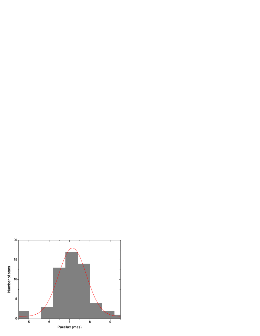
Figure 15: Histogram of the parallaxes for group members with known radial velocities. The superimposed curve represents a Gaussian fit to the data.

Table 5 lists the name and HBC number, as well as the values of the derived Galactic coordinates (Columns 3 to 5) and Galactic velocity components with their uncertainties (Columns 6 to 8) for the 67 members of the moving group – both core members and confirmed candidates (see Sect.5.4 below) – with known radial velocities, i.e., those stars for which the derived parallaxes are most accurate. This table can be used to identify individual group members in the figures.

Figure 12 displays the projected velocities on the $XY$, $XZ$, and $YZ$ planes for the 67 same group members. Figure 13 shows their spatial distribution. The stars are distributed in a $X,Y,Z$ cube with sides of approximately 60pc, and filamentary structure, reminiscent of the Taurus molecular cloud structure, can be seen in all three $(X,Y)$, $(Y,Z)$, and $(X,Z)$ projection planes. In the $(X,Z)$ plane, there is some tendency for the densest subgroups of stars to align roughly in the direction away from the Sun. This is an expected result of the changed parallax values, since the stars must maintain their apparent distribution in the plane of the sky, as seen from Earth. Note that individual stars can be identified by their coordinate values given in Table 5. Finally, Fig. 14 displays histograms of the $U,V,W$ galactic velocity components and spatial velocities of the members of the Taurus moving group with known radial velocities.

Table 6: Tentative parallaxes (in mas) and distances (in pc) of 25 moving group stars with unknown radial velocities computed under the assumption that they share the same spatial velocity.

Star	HBC	$\pi_{Vspace}\pm\sigma_{\pi}$	$d_{Vspace}\pm\sigma_{d}$
LkCa 1	365	8.86 $\pm$ 2.69	113 ${}^{+49}_{-26}$
FN Tau	24	9.64 $\pm$ 2.84	104 ${}^{+43}_{-24}$
LkCa 3	368	5.89 $\pm$ 2.16	170 ${}^{+98}_{-46}$
FO Tau	369	6.76 $\pm$ 2.12	148 ${}^{+68}_{-35}$
V892 Tau	373	8.70 $\pm$ 2.51	115 ${}^{+47}_{-26}$
Haro 6-5B	381	5.19 $\pm$ 2.31	193 ${}^{+154}_{-59}$
FS Tau	383	5.10 $\pm$ 2.30	196 ${}^{+161}_{-61}$
LkCa 21	382	8.72 $\pm$ 2.52	115 ${}^{+46}_{-26}$
FV Tau/c	387	8.76 $\pm$ 2.91	114 ${}^{+57}_{-28}$
DG Tau	37	6.82 $\pm$ 1.75	147 ${}^{+51}_{-30}$
ZZ Tau	46	8.53 $\pm$ 2.71	117 ${}^{+55}_{-28}$
LkH$\alpha$ 358	394	5.91 $\pm$ 2.73	169 ${}^{+145}_{-53}$
XZ Tau	50	7.25 $\pm$ 1.89	138 ${}^{+48}_{-28}$
Haro 6-13	396	6.30 $\pm$ 2.56	159 ${}^{+108}_{-46}$
FY Tau	401	3.52 $\pm$ 1.70	284 ${}^{+263}_{-92}$
FZ Tau	402	10.51 $\pm$ 2.95	95 ${}^{+37}_{-21}$
UZ Tau AB	52	7.43 $\pm$ 2.49	135 ${}^{+68}_{-34}$
V807 Tau	404	6.57 $\pm$ 1.70	152 ${}^{+53}_{-31}$
IS Tau	59	8.34 $\pm$ 2.65	120 ${}^{+56}_{-29}$
HO Tau	64	5.84 $\pm$ 2.31	171 ${}^{+112}_{-49}$
FF Tau	409	5.80 $\pm$ 2.30	172 ${}^{+113}_{-49}$
CoKu Tau-Aur Star 3	411	9.16 $\pm$ 3.04	109 ${}^{+54}_{-27}$
CoKu HP Tau G2	415	5.38 $\pm$ 1.44	186 ${}^{+68}_{-39}$
CoKu LkH$\alpha$ 332 G1	423	8.73 $\pm$ 2.42	115 ${}^{+44}_{-25}$
DP Tau	70	6.54 $\pm$ 2.36	153 ${}^{+87}_{-41}$

5.3.2 Approximate parallaxes for other moving group members

We now assume that all members of the moving group share the same average value of $V_{space}$ derived above. This hypothesis allows us to compute expected radial velocities for all stars in the moving group and subsequently to derive tentative parallaxes for those group members.

Figure 16 compares the parallax values obtained by both methods and shows that they give similar results within the error bars, but the scatter is large. There is also a bias in the derived parallaxes in the sense that small parallaxes are underestimated, and large parallaxes are overestimated, when determined from the group spatial velocity, as shown by the linear fit to the data (dotted line in Fig. 16). According to this regression curve, the parallax average and standard deviation computed using radial velocities, $6.99\pm 1.14$ mas, translate to $6.74\pm 1.44$ mas when using the average spatial velocity for computing the parallax; not only is the resulting parallax smaller on average but its standard deviation is larger. The parallaxes deviating most from the mean in Table 6 should therefore be viewed with extreme caution. A case in point is the couple FY/FZ Tau, two stars separated by less than 20^′′ on the sky whose derived parallaxes are respectively the smallest and the largest of our sample. The result for FY Tau is obviously unrealistic, as both stars are seen in projection on the B18 nebula and have the same line-of-sight visual extinction.

The average parallax and associated standard deviation of stars in Table 6 are $\pi=7.21\pm 1.71$ mas, corresponding to an average distance of 139 pc. The average distance of these stars is similar to that of stars for which we know the radial velocities, but the parallax standard deviation is almost twice as large, as anticipated from the regression analysis. Although the derived parallaxes can only be considered as tentative and would be much improved, and their uncertainties reduced, if accurate spectroscopic radial velocities were available for the full sample, this approximation nevertheless may provide a useful first estimate of the distance to those moving group members whose parallax is not too different from the mean (e.g., DG Tau, XZ Tau, and UZ Tau).

5.4 Additional group member candidates

After finding a core moving group among the pre-main sequences stars of Taurus-Auriga, we now look for plausible additional members among stars in the Ducourant et al. (2005) catalog whose evolutionary status is uncertain. We thus now consider the full sample of 217 stars discussed in Sect. 2 and identify those whose space motion is compatible with that of the core moving group.

5.4.1 Analysis and results

Specifically, we assumed that the CP of the entire moving group has the coordinates found above for the core moving group and computed the individual probability of each star being part of the moving group converging to this point by using Eq. 9. A $p_{min}$ minimum value of 0.91 was chosen because it is the lowest value to allow for the rejection of all those stars in the subgroup of confirmed PMS objects that are not actual members of the core moving group. Stars with a lower $p_{min}$ were thus eliminated, leaving us with 30 stars whose space motion is compatible with that of the core moving group.

Among these 30 objects, 15 have known radial velocities; their parallaxes are given in Table 7 and the kinematic properties of confirmed members (see below) are listed in Table 5. As previously, we computed the spatial velocity of this sample to compute approximate parallaxes for the remaining 15 stars, and we give these tentative parallaxes in Table 8.

Table 7: Parallaxes (in mas), distances (in pc), and probable evolutionary status of 15 possibly additional moving group stars with known radial velocities. Parallaxes of stars that are not PMS members of Taurus-Auriga are meaningless and are therefore not given here.

Star	$\pi_{Vspace}\pm\sigma_{\pi}$	$d_{Vspace}\pm\sigma_{d}$	PMS
RX J0400.5+1935			n
GSC 01262-00421	6.03 $\pm$ 0.88	166 ${}^{+28}_{-21}$	y
RX J0405.7+2248	5.69 $\pm$ 0.87	176 ${}^{+32}_{-23}$	y
RX J0406.7+2018	6.30 $\pm$ 0.95	159 ${}^{+28}_{-21}$	y
RX J0406.8+2541			n
RX J0423.7+1537	7.56 $\pm$ 1.08	132 ${}^{+22}_{-16}$	y
RX J0424.8+2643B			n
RX J0432.8+1735	6.47 $\pm$ 2.37	155 ${}^{+89}_{-41}$	y
V1078 Tau	3.87 $\pm$ 0.71	259 ${}^{+58}_{-40}$	y
RX J0444.9+2717			n
RX J0450.0+2230			n
RX J0452.5+1730	7.24 $\pm$ 2.62	138 ${}^{+78}_{-37}$	y
RX J0455.8+1742			n
RX J0457.0+1517	8.22 $\pm$ 1.13	122 ${}^{+19}_{-15}$	y
RX J0457.5+2014	7.44 $\pm$ 1.06	134 ${}^{+22}_{-17}$	y

Table 8: Tentative parallaxes (in mas), distances (in pc), and probable or tentative evolutionary status of 15 possibly additional moving group stars with unknown radial velocities. Parallaxes of stars that are not PMS members of Taurus-Auriga are meaningless and are therefore not given here. Confirmation of PMS status is required for most objects.

Star	$\pi_{Vspace}\pm\sigma_{\pi}$	$d_{Vspace}\pm\sigma_{d}$	PMS
1RXS J035330.5+263152			n
RX J0412.8+2442			n
KPNO-Tau 11	8.15 $\pm$ 2.75	123 ${}^{+63}_{-31}$	y
FR Tau	7.25 $\pm$ 2.58 (?)	138 ${}^{+76}_{-36}$ (?)	y?
FU Tau	8.44 $\pm$ 2.87 (?)	118 ${}^{+61}_{-30}$ (?)	y?
FW Tau	6.81 $\pm$ 2.58 (?)	147 ${}^{+89}_{-40}$ (?)	y?
RX J0431.3+2150	4.39 $\pm$ 1.23	228 ${}^{+89}_{-50}$	y
EZ Tau			n
FI Tau	7.61 $\pm$ 2.79 (?)	131 ${}^{+76}_{-35}$ (?)	y?
GN Tau	6.07 $\pm$ 2.50 (?)	165 ${}^{+115}_{-48}$ (?)	y?
Haro 6-36	5.83 $\pm$ 2.59 (?)	171 ${}^{+137}_{-53}$ (?)	y?
Haro 6-39	7.92 $\pm$ 2.88 (?)	126 ${}^{+72}_{-34}$ (?)	y?
RX J0456.6+3150	2.68 $\pm$ 0.84 (?)	373 ${}^{+170}_{-89}$ (?)	?
1RXS J050029.8+172400	4.92 $\pm$ 1.39 (?)	203 ${}^{+80}_{-45}$ (?)	y?
1RXS J051111.1+281353	6.82 $\pm$ 1.75 (?)	147 ${}^{+51}_{-30}$ (?)	?

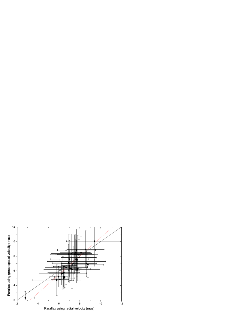
Figure 16: Comparison of parallaxes computed using the radial velocity data and the group spatial velocity derived from the subgroup of stars with known radial velocities. The solid line indicates perfect correlation, while the dotted line represents a linear fit to the data.

5.4.2 Evolutionary status of candidate members

The ROSAT-detected stars included in Table 7 were studied in some detail by Wichmann et al. (2000), who assessed their evolutionary status on the basis of their lithium line strengths. The two other stars, GSC 01262-00421 and V1078 Tau, were studied by Walter et al. (1988), who concluded, also from their lithium strength, that they were bona fide PMS objects. A “y” in last column of Table 7 indicates that the star is a PMS object on the basis of these two works. We thus find that 9 of of the 15 stars are confirmed PMS objects and thus members of the Taurus-Auriga moving group.

Most stars included in Table 8 have not been studied in any kind of detail, so assessing their evolutionary status on the basis of the available information is a challenge. All stars marked with “y?” in the last table column are IRAS point sources (Strom et al. 1989) and are therefore likely to be associated with circumstellar matter, which strongly hints at PMS status; however, spectroscopic confirmation is unavailable. 1RXS J035330.5+263152 is the X-ray counterpart of a likely member of the Pleiades corona (Pels et al. 1975), while RX J0412.8+2442 is unlikely to be young according to Magazzù et al. (1997). KPNO-Tau 11 is a recently-detected low-mass member of the Taurus star-forming region (Luhman et al. 2003), while RX J0431.3+2150 was originally proposed as a PMS object by Wichmann et al. (1996), and this status was confirmed by Bouvier et al. (1997). EZ Tau is a flare star and probable low-mass member of the Hyades (Reid 1993). 1RXS J050029.8+172400 was classified as a T Tauri star on the basis of its X-ray variability by Fuhrmeister & Schmitt (2003), but this needs to be confirmed by optical spectroscopy. Finally, there is not enough information to assess the status of RX J0456.6+3150 and 1RXS J051111.1+281353. The second star was classified as T Tauri star by Li (2004) on the basis of its proper motion, but we have seen that this criterion is not discriminatory. Altogether, only 2 of these 15 stars are confirmed members of the moving group, while 8 are possibly additional members.

5.5 Note on X-ray selected stars located south of Taurus

Finally, we searched for putative moving group members in the region south of Taurus where a large population of X-ray sources possibly related to the Taurus-Auriga star-forming region was detected by the ROSAT All-Sky X-ray survey (Magazzù et al. 1997). We thus considered the region $3^{h}50^{m}$ $\;\buildrel<\over{\sim}\;$$\alpha(2000)$ $\;\buildrel<\over{\sim}\;$$5^{h}10^{m}$ and $0$^∘$\;\buildrel<\over{\sim}\;$$\delta(2000)$ $\;\buildrel<\over{\sim}\;$$15$^∘, where the Ducourant et al. (2005) catalog lists 47 stars, and did the same analysis as in Sect. 5.4 thus searching for additional members of the core moving group defined in Sect. 5.3. In this way, we identified 7 stars whose space motion is compatible with that of the core moving group. These are RX J0357.3+1258, RX J0358.1+0932,RX J0404.4+0519, RX J0450.0+0151, RX J0405.5+0324, RX J0441.9+0537, and RX J0445.3+0914.

Since the kinematic analysis is not sufficient for identifying moving group members with any kind of certainty, we searched the literature to determine the evolutionary status of these objects. The first four objects were studied among other PMS candidates by Neuhäuser et al. (1997), who found that RX J0450.0+0151 is a likely PMS star while the other stars are on the main sequence. The remaining stars are part of a sample studied by Magazzù et al. (1997), who list them as main sequence objects.

With the possible exception of RX J0450.0+0151, for which we derive a parallax of $11.84\pm 1.33$ mas corresponding to a distance of $84^{+11}_{-9}$ pc, we thus conclude that the X-ray sources located south of Taurus that have proper motions compatible with those of the core Taurus-Auriga moving group are field stars unrelated to the Taurus-Auriga PMS association.

5.6 A posteriori assessment of results

To assess the validity of the results presented above, we performed additional Monte Carlo simulations of the core moving group search using the results derived above. For this, we constructed synthetic data sets as explained in Sect. 4; but instead of drawing a random velocity vector, we used the velocity of the moving group as derived from the CP search, i.e., $V_{group}=7.3$ km/s, $\Theta=116$^∘, and $\Phi=171$^∘. To define the individual velocity of each synthetic star, we added to the group velocity vector an individual random velocity drawn from a normal distribution with variance $\sigma_{int}$ and derived the resulting proper motions and radial velocities from there. We then added random measurements errors and corrected for the Galactic rotation as explained in Sect. 4. Because the considered sample of 117 Taurus-Auriga stars used in the CP search is made up of confirmed pre-main sequence stars, we did not include interlopers in these simulations.

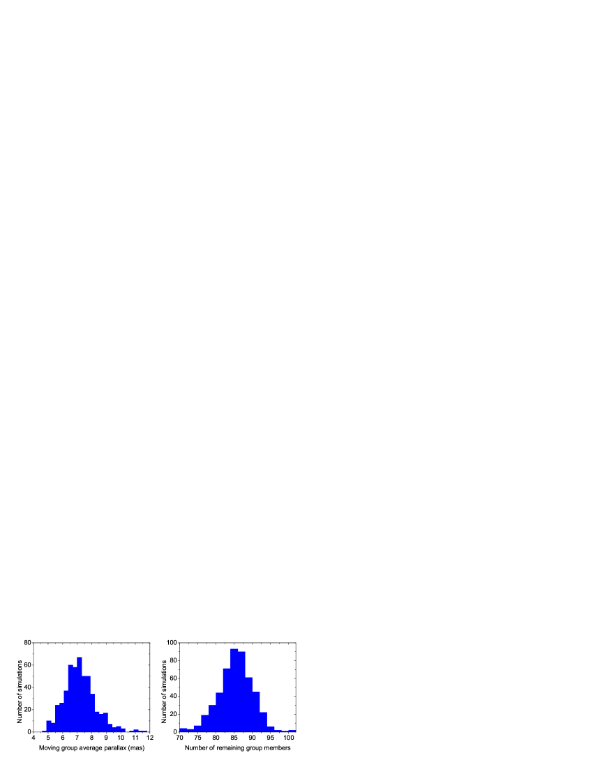
Figure 17: Results of simulations performed with the computational parameters used in Sect. 5. Histograms of the recovered average parallaxes and of the numbers of recovered group members are shown.

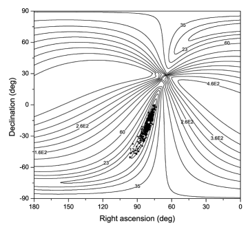
Figure 18: Realizations of CP coordinates (dots) in the Monte-Carlo simulation, overlaid on the $X^{2}$ contours for the core moving group solution derived in Sect. 5. The white star denotes the CP coordinates of the Taurus-Auriga core moving group as derived in that section.

We constructed 500 such realizations in our simulation, which we ran with the same computational parameters as the actual CP search of Sect. 5. The results of these simulations are illustrated by Fig. 17, which demonstrates that the probability of recovering the average parallax of a moving group with Taurus-Auriga properties is 0.38 and that the average number of stars in the recovered moving group is $85\pm 5$, whereas we found 83 members for the core moving group in the actual solution. The probability that the CP method cannot find a moving group in this situation is 0.05. The histogram of derived parallaxes can be fitted by a Gaussian curve peaking at $7.06\pm 0.04$ mas with HWHM equal to $0.86\pm 0.06$ mas, whereas the input values for these two quantities were respectively 7.31 and 0.49 mas. Our actual computation recovers the average parallax of Taurus because we hit on one of the best possible solutions for the CP coordinates, as shown below.

The derived CP coordinates in the 500 simulations are shown in Fig. 18. As previously discussed, e.g., by de Bruijne (1999) CP coordinates fall along the great circle associated with the CP, which is accurately defined by the proper motions, but the precise location of the CP on this great circle is quite uncertain. For comparison, we also plot in Fig. 18 the $X^{2}$ values (as defined by Eq. 10) that measure the probability of finding the CP at a given location on the plane of the sky. The curves plotted here correspond to the solution found in Sect. 5, and the white star indicates the coordinates of the derived Taurus-Auriga core moving group CP. The topology of the $X^{2}$ surface seen here is typical of the CP method. A large fraction of the sky forms a high plateau (in terms of $X^{2}$) cut by a deep valley following the great circle associated with the CP, with an elongated minimum following the great circle at the location of the CP. The height of the plateau and the depth of the valley are directly related to the velocity dispersion and measurements uncertainties in the sense that reducing these values increases the contrast between plateau and valley, thus making it easier to locate the CP precisely.

The lowest $X^{2}$ contour in Fig. 18 corresponds to a value of 13 and includes most CP realizations. With an $X^{2}$ of 10.6, the coordinates of the CP derived for Taurus-Auriga obviously represent one of the best possible solutions, thus validating the choice of computational parameters used to find it. However, we expect only 73% of the actual moving group members to be recovered in the computation. Therefore, most stars in our core sample are likely to be actual members of the moving group even though they were rejected during the CP search. In order to identify these potentially additional moving group members and derive their individual parallaxes, more precise radial velocities and proper motions will be necessary.

6 Remarks on positions and parallaxes

A first check of our results is provided by a comparison with Hipparcos parallaxes.

6.1 Comparison with Hipparcos results

As already mentioned in Sect. 2, there is little overlap between Taurus YSOs and Hipparcos targets, due mainly to the faintness of most Taurus PMS stars. We found 11 stars among our moving group that have been observed by Hipparcos and listed them in Table 9, together with the parallaxes derived in this work and the Hipparcos parallaxes. The values agree within the error bars except for 3 objects: BP Tau, DF Tau, and UX Tau, for which Hipparcos reports a negative parallax. The discrepant Hipparcos parallaxes of BP Tau and DF Tau were discussed in some detail by Bertout et al. (1999), who concluded from a re-analysis of the Hipparcos data that the derived large parallaxes were unlikely to be significant, although they could not be ruled out entirely. Bertout et al. (1999) also re-computed a more precise parallax of $7.98\pm 3.15$ mas for RW Aur after rejecting the bad abscissae. We thus conclude that there is a general agreement between the parallaxes derived here and the Hipparcos values except for BP Tau and DF Tau. The values reported in this work for these two objects are much more in line with expectations than the Hipparcos values, since the two stars are clearly associated with the molecular cloud.

Table 9: Comparison with Hipparcos catalog parallaxes. Units are mas.

Name	HIP	HBC	$\pi_{Vrad}\pm\sigma_{\pi}$	$\pi_{HIP}\pm\sigma_{\pi}$
V773 Tau	19762	367	6.84 $\pm$ 1.07	9.88 $\pm$ 2.71
V410 Tau	20097	29	7.3 $\pm$ 0.88	7.31 $\pm$ 2.07
BP Tau	20160	32	7.46 $\pm$ 0.66	18.98 $\pm$ 4.65
RY Tau	20387	34	7.62 $\pm$ 0.68	7.49 $\pm$ 2.18
HD 283572	20388	380	7.64 $\pm$ 1.05	7.81 $\pm$ 1.3
DF Tau	20777	36	7.76 $\pm$ 1.29	25.72 $\pm$ 6.36
UX Tau	20990	43	6.55 $\pm$ 0.99	-6.68 $\pm$ 4.04
AB Aur	22910	78	8.79 $\pm$ 1.48	6.93 $\pm$ 0.95
SU Aur	22925	79	6.99 $\pm$ 0.73	6.58 $\pm$ 1.92
RW Aur	23873	80	7.21 $\pm$ 0.82	14.18 $\pm$ 6.84
RX J0406.7+2018	19176	-	6.3 $\pm$ 0.95	6.43 $\pm$ 1.84

Figure 19: Location of the moving group stars in the plane of the sky. As indicated in the legend, different symbols mark the stars closer than 130pc, those farther away than 155pc, and the remaining stars.

We restrict the following discussion to those members of the moving group with measured radial velocities since we derived accurate parallaxes for these objects, whereas the parallaxes derived for other stars from the group’s average spatial velocity are tentative.

6.2 Notes on remarkable stars

NTTS 035120+3154 (HBC 352/353) provides an interesting illustration of the current limitations of the study reported here. According to Leinert et al. (1993), the SW and NE components of this object are likely to form a physical pair. The proper motions and radial velocities of both stars, given in Table 10, agree within the error bars; and yet, we derive distances (see Table 4) that, while they agree with each other within the derived error bars, differ by 34 pc, i.e., 14% of the mean distance value of 242 pc. This uncertainty thus appears representative of what can be done with the current data. Assuming that the radial velocities were equal within 0.1 km/s, one finds that the gap between distances is reduced to 22 pc, or 9% of the mean distance. This increased accuracy is thus within easy reach since it only requires accurate radial velocities. On the other hand, this also shows that without much more accurate proper motions measurements, the uncertainty on derived distances cannot be expected to decrease much below 10%.

Table 10: Proper motions (in mas/yr) and radial velocity (in km/s) for NTTS 035120+3154

Name	$\mu_{\alpha}\cos\delta\pm\sigma_{\mu}$	$\mu_{\delta}\pm\sigma_{\mu}$	$V_{rad}\pm\sigma_{V}$
NTTS 035120+3154SW	8 $\pm$ 2	-9 $\pm$ 2	16.0 $\pm$ 1.5
NTTS 035120+3154NE	7 $\pm$ 2	-11 $\pm$ 2	15.1 $\pm$ 1.5

NTTS 042835+1700 (HBC 392) appears to be the closest star in the moving group at 106 pc (2.1$\sigma$ from the average moving group distance), while NTTS 043124+1824 (HBC 407) is the farthest away at 360 pc, i.e., 3.7$\sigma$ away from the average. The proper motion values of HBC 407, an apparently single star (König et al. 2001), are indeed very small, with $\mu_{\alpha}\cos\delta=0\pm 2$ mas/yr and $\mu_{\delta}=-7\pm 2$ mas/yr. Its radial velocity of 18.4 km/s is not very different from the average of 16 km/s and it is therefore difficult to understand how the star could have reached this location in space if it is a true member of the Taurus-Auriga moving group. Its PMS nature has been confirmed by Walter et al. (1988) and others, and it is thus unlikely to be an interloper. Its discrepant parallax, if true, remains therefore somewhat of a mystery, but we note that the computed uncertainty on its value is particularly high.

CZ Tau (HBC 31) is another interesting case because it is located at less than 20^′′  from DD Tau and has the same proper motion yet its radial velocity is highly discrepant (compared to the Taurus-Auriga average) at 44 km/s. The radial velocity measurements for both objects go back to the classic paper where Joy (1949) discussed the class of T Tauri stars for the first time, and they are noted as very uncertain in the Herbig & Bell (1988) catalog. The derived parallaxes are therefore also very uncertain so we marked them as such in Table 4.

6.3 Properties of parallaxes for various YSO sub-classes

Figure 19 displays the members of the moving group as seen in the plane of the sky. The moving group contains 23 classical T Tauri stars (CTTSs) and 43 confirmed weak emission-line T Tauri stars (WTTSs) with known radial velocities. Among the WTTSs, we have 18 X-ray selected WTTSs (XWTTSs) and 25 optically-selected WTTSs (OWTTSs). A comparison of the parallaxes of stars in these subgroups confirms that X-ray selected WTTSs tend to be found on the outskirts of the molecular clouds where extinction is relatively low, while CTTSs (and OWTTSs) are associated with the denser regions of the clouds (see also the parallax histograms of the various YSO populations in Fig. 20).

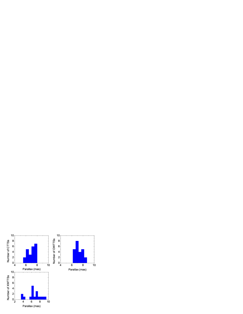
Figure 20: Histograms of parallaxes computed using the radial velocities for the sub-samples of CTTSs, OWTTSs, and XWTTSs in the moving group.

An interesting, although not unexpected new finding of our investigation is that WTTSs are located not only in front of the clouds, but also at their back, while CTTSs are confined to the central parts of the moving group. This is illustrated by Fig. 20, which displays histograms of the CTTS and WTTS parallaxes. All CTTSs are at distances between 126 and 173 pc, while WTTSs span the range of distances between 106 and 259 pc.

Computing average parallaxes and standard deviations for these various subgroups, we get

$$\overline{\pi_{CTTS}} = 7.01\pm 0.67{\rm mas}$$

$$\overline{\pi_{WTTS}} = 7.00\pm 1.15{\rm mas}$$

$$\overline{\pi_{OWTTS}} = 7.28\pm 0.65{\rm mas}$$

$$\overline{\pi_{XWTTS}} = 6.60\pm 1.55{\rm mas},$$

where we note that the standard deviation of the XWTTS parallaxes is more than twice as large as those of CTTSs and OWTTSs.

For the sample of CTTSs and OWTTSs with known radial velocities, the individual parallaxes of which are presumably more accurate than those computed from the group spatial velocity, we recover the average parallax value derived by Bertout et al. (1999) from Hipparcos data. Our analysis thus confirms that the core of the Taurus association, as defined by this CTTS and OWTTS sample, is located at $140^{+14}_{-12}$ pc.

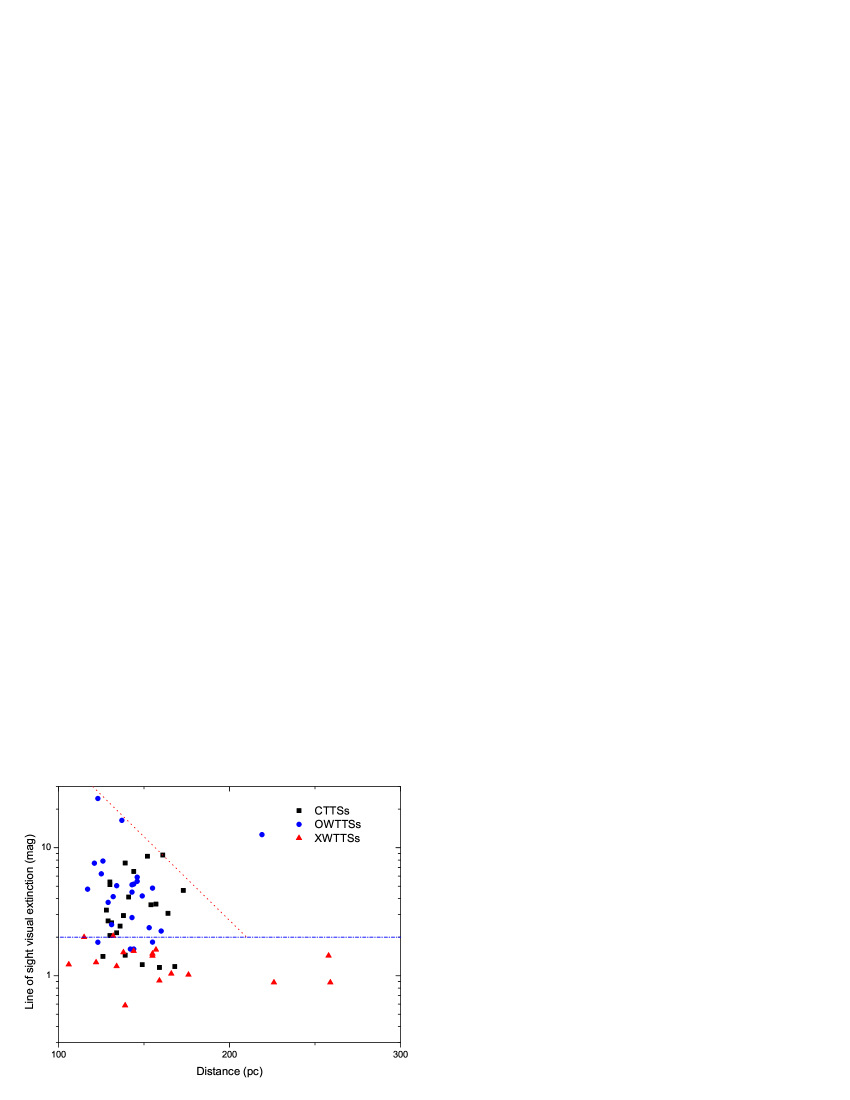
Figure 21: Line-of-sight visual extinction of moving group members plotted as a function of their distance. Different symbols, shown in the legend, are used to identify X-ray selected WTTSs (XWTTSs), optically selected WTTSs (OWTTSs), and CTTSs. The meaning of the two lines is discussed in the text.

That we are actually observing WTTSs on both sides of the molecular clouds may seem at first to contradict the idea that X-ray selected stars tend to be detected in low-extinction regions. However, one must recall that extinction is very patchy in the Taurus-Auriga star-forming region, characterized by a dense filamentary structure and zones of lower molecular gas density. To test whether XWTTSs are indeed preferentially found along low-extinction lines of sight, we used the extinction maps of Schlegel et al. (1998) to derive the line-of-sight (LOS) visual extinction in the direction of each moving group star. Figure 21 shows that XWTTSs are on the average located on lines of sight that have lower visual extinctions than OWTTSs and CTTSs. The horizontal dash-dotted line indicates the upper limit of LOS extinction for XWTTSs of 2 mag. Not surprisingly, there is no significant difference between the LOS extinctions of OWTTS and CTTS subgroups. Note that no star farther away than $\approx 180$ pc (except for one star, CZ Tau, the parallax of which is highly uncertain as discussed above) has a LOS extinction higher than 1.5 magnitudes. The upper envelope of the data points in Fig. 21 (dotted line) indicates approximately how far one “sees” in the Taurus star-forming region for a given LOS extinction. Lines of sight where the extinction is in the range $2\leq A_{V}\leq 20$ mag. become opaque in the optical domain at distances in the range $210\geq d\geq 120$ pc. From these numbers, and using the conversion factor from extinction to hydrogen column density given by Predehl & Schmitt (1995), one finds an average hydrogen density of $\approx 2\cdot 10^{2}$ cm^-3 in Taurus, a value that agrees with expectations for large molecular clouds.

7 Conclusions

We have identified a moving group of 94 stars in the Taurus-Auriga association that defines the kinematic properties of the T association. Because the variant of the CP search method that we developed for dealing with the high internal velocity dispersion among Taurus subgroups possibly eliminates a number of potential group members, we detected a minimum moving group that may not contain all the kinematically associated stars in the region.

Determination of accurate parallaxes for all moving group members is hampered by the lack of observed high-precision radial velocities for many group members. New radial velocity measurements for all stars of the Ducourant et al. (2005) proper-motion catalog are obviously needed in order to make further progress in deriving accurate parallaxes for individual YSOs in T associations. We therefore encourage observers to make use of the highly efficient and precise spectrographs employed, in particular, for extra-solar planet searches to perform a complete radial velocity survey of Taurus-Auriga and other star-forming regions.

The present result nevertheless represents a first step towards better understanding the distances to Taurus-Auriga PMS stars, and we use these new distances to re-assess the physical properties of members of the Taurus-Auriga moving group in a companion paper (Bertout & Siess, in preparation).