Stellar magnetosphere reconstruction from radio data
Abstract
Aims. In order to fully understand the physical processes in the magnetospheres of the Magnetic Chemically Peculiar stars, we performed multi-frequency radio observations of CU Virginis. The radio emission of this kind of stars arises from the interaction between energetic electrons and magnetic field. Our analysis is used to test the physical scenario proposed for the radio emission from the MCP stars and to derive quantitative information about physical parameters not directly observable.
Methods. The radio data were acquired with the VLA and cover the whole rotational period of CU Virginis. For each observed frequency the radio light curves of the total flux density and fraction of circular polarization were fitted using a three-dimensional MCP magnetospheric model simulating the stellar radio emission as a function of the magnetospheric physical parameters.
Results. The observations show a clear correlation between the radio emission and the orientation of the magnetosphere of this oblique rotator. Radio emission is explained as the result of the acceleration of the wind particles in the current sheets just beyond the Alfvén radius, that eventually return toward the star following the magnetic field and emitting radiation by gyrosyncrotron mechanism. The accelerated electrons we probed with our simulations have a hard energetic spectrum () and the acceleration process has an efficiency of about . The Alfvén radius we determined is in the range of and, for a dipolar field of 3000 Gauss at the magnetic pole of the star, we determine a mass loss from the star of about M☉ yr-1. In the inner magnetosphere, inside the Alfvén radius, the confined stellar wind accumulates and reaches temperatures in the range of K, and a detectable X-ray emission is expected.
Key Words.:
stars: chemically peculiar – stars: circumstellar matter – stars: individual: CU Vir – stars: magnetic field – stars: mass loss – radio continuum: stars1 Introduction
Magnetic Chemically Peculiar (MCP) stars are characterized by periodic variability of the effective magnetic field through the stellar rotational period. The magnetic field topology of this kind of star has been commonly regarded as a magnetic dipole tilted with respect to the rotation axis (Babcock b49 (1949); Stibbs s50 (1950)), even if MCP stars with a multipolar magnetic field are also known (Landstreet l90 (1990); Mathys m91 (1991)).
In some cases, MCP stars are characterized by an anisotropic stellar wind (Shore et al. s_etal87 (1987); Shore & Brown sb90 (1990)), as a consequence of the wind interaction with the dipolar magnetic field (Shore s87 (1987)). The resulting magnetosphere is structured in a “wind zone” at high magnetic latitudes, where the gas flows draw the magnetic field out to open structures, and a “dead zone”, where the magnetic field topology is closed and the gas trapped.
| UT | UT | UT | ||||||||
| [mJy] | [mJy] | [mJy] | [mJy] | [mJy] | [mJy] | |||||
| Date: 1998 June 02 | ||||||||||
| 00:30:45 | 01:37:00 | 02:51:50 | ||||||||
| 01:23:05 | 02:36:55 | 03:51:35 | ||||||||
| 02:22:55 | 03:38:50 | 04:51:25 | ||||||||
| 03:22:45 | 04:36:35 | 05:51:20 | ||||||||
| 04:22:35 | 05:36:30 | 06:51:15 | ||||||||
| 05:22:25 | 06:36:20 | 07:44:20 | ||||||||
| 06:22:15 | 07:30:25 | … | … | … | ||||||
| 07:18:55 | … | … | … | … | … | … | ||||
| 08:13:45 | … | … | … | … | … | … | ||||
| Date: 1998 June 07 | ||||||||||
| 02:10:15 | 02:23:40 | 02:38:10 | ||||||||
| 03:08:35 | 03:21:35 | 03:35:55 | ||||||||
| 04:06:25 | 04:19:25 | 04:33:45 | ||||||||
| 05:04:50 | 05:18:20 | 05:32:45 | ||||||||
| 06:03:35 | 06:17:05 | 06:31:35 | ||||||||
| 07:02:30 | 07:15:15 | … | … | … | ||||||
| 07:54:30 | … | … | … | … | … | … | ||||
| Date: 1998 June 12 | ||||||||||
| 01:21:35 | 01:35:05 | 02:47:25 | ||||||||
| 02:19:55 | 02:32:55 | 03:45:15 | ||||||||
| 03:17:45 | 03:30:45 | 04:44:10 | ||||||||
| 04:16:05 | 04:29:35 | 05:43:00 | ||||||||
| 05:15:05 | 05:28:25 | 06:41:50 | ||||||||
| 06:13:55 | 06:27:20 | … | … | … | ||||||
| 07:09:30 | 07:20:55 | … | … | … | ||||||
Currently, non-thermal radio emission is observed from about 25% of MCP stars and the detection rate seems to be directly correlated to the effective stellar temperature (Drake et al. d_etal87 (1987); Linsky et al. l_etal92 (1992); Leone et al. l_etal94 (1994)). Since only MCP stars with high photospheric temperature develop a radiatively-driven stellar wind, this result reveals the importance of a stellar wind in driving the radio emission. To explain the origin of the radio emission from pre-main sequence magnetic B stars and from MCP stars, André et al. (a_etal88 (1988)) proposed a model characterized by the interaction between the wind and the magnetic field. The radio emission is understood in terms of gyrosynchrotron emission from mildly relativistic electrons, which are accelerated in “current sheets” formed where the gas flow brakes the magnetic field lines, close to the magnetic equator plane, and propagate along the magnetic field lines back to the inner magnetospheric regions (Havnes & Goertz hg84 (1984); Usov & Melrose um92 (1992)).
According to the oblique dipole model, Leone (l91 (1991)) suggested that the radio emission of MCP stars should be also periodically variable. The confirmation of this hypothesis comes from the observations of HD37017 and HD37479 (Leone & Umana lu93 (1993)) and of HD133880 (Lim et al. l_etal96 (1996)), performed at 5 GHz, that revealed the presence of rotational flux modulation. In particular, the observed flux light curves of HD37017 and HD37479, which are characterized by a simple dipolar magnetic field, show a radio emission minimum coincident with the zero of the longitudinal magnetic field, whereas the emission is maximum at the magnetic field extrema.
Among radio MCP stars, only CU Virginis (HD124224) is characterized by a strong 1.4 GHz flux enhancement around phases 0.4 and 0.8, with a right hand circular polarization of almost 100% (Trigilio et al. t_etal00 (2000), TLL00). This discovery has been explained in terms of Electron Cyclotron Maser Emission (ECME) from energetic electrons accelerated in the current sheets near the Alfvén surface (where the thermal plus kinetic plasma pressure equals the magnetic one) and reflected outward by magnetic mirroring in the inner magnetospheric layers.
In a previous paper (Trigilio et al. t_etal04 (2004), TLU04), we developed a three-dimensional numerical model of the radio emission from MCP stars with a dipolar field. On the basis of successfull simulated 5 GHz flux light curves of HD37017 and HD37479, whose study allowed us to confirm the qualitative scenario proposed to explain the origin of non-thermal radio emitting electrons. We showed that the combined effect of a tilted dipolar magnetic topology and the presence of a thermal plasma trapped in the “dead-zone” can produce the observed phase modulation of the stellar radio emission.
In this paper we present the multifrequency microwave observations of CU Virginis, a well studied Si-group MCP star.


To investigate the physical conditions of the stellar magnetosphere, the radio light curves of CU Vir are compared with the results of the numerical simulations performed using our 3D model. We present here an implementation of our code to also treat circular polarization.
2 Observations and data reduction
The observations were carried out using the VLA111The Very Large Array is a facility of the National Radio Astronomy Observatory which is operated by Associated Universities, Inc. under cooperative agreement with the National Science Foundation. in three different runs, on June 02, 07 and 12, 1998. Each run was approximately eight hours long. We observed at four frequencies (1.4, 5, 8.4 and 15 GHz) using two independent and contiguous bands of 50 MHz in Right and Left Circular Polarizations (RCP and LCP). The observations were performed using the entire array (configuration array moving A B) alternating all the frequencies.
Because of the rotational period and with the aim to obtain a complete rotational phase coverage, we assumed at any frequency an observing cycle consisting of 10 minutes on source, preceded and followed by 2 minutes on the phase calibrator (). To avoid redundancy in the phase coverage for each frequency, the observing sequence was changed in each run.
The flux density scale was determined by daily observations of 3C286. The data were calibrated and mapped using the standard procedures of the Astronomical Image Processing System (AIPS). The flux density and fraction of circular polarization were obtained by fitting a two-dimensional Gaussian, task JMFIT, at the source position in the cleaned maps (separately for the Stokes and Stokes 222VLA measurements of wave polarization state are in agreement with the IAU and IEEE orientation/sign convention: positive V corresponds to right circular polarization.) integrated over the duration of each individual scan. As the uncertainty in the flux density measurements we assume the r.m.s. of the map. Results are summarized in Table 1. The measurements performed at 1.4 GHz have been presented elsewhere (TLL00).
3 The radio behavior of CU Vir
In Fig. 1, for each observed frequency, we report the radio flux density
measured in both Stokes and versus the
rotational phase. This was computed adopting the ephemeris referred to light minimum
reported by Pyper et al. (p_etal98 (1998)):
In the lowest panel of Fig. 1 the measures performed in Stokes at 1.4 GHz from TLL00 are also displayed.
The top panel of Fig. 1 shows the average longitudinal component of the magnetic field as a function of the rotational phase (data are from Borra & Landstreet bl80 (1980) and Pyper et al. p_etal98 (1998)).
The flux variability with the stellar rotational period suggests that the radio emission at 15, 8.4 and 5 GHz arises from a stable co-rotating magnetosphere and that the radio source is optically thick. For Stokes the radio emission minimum appears to be coincident with the null magnetic field ( and ), whereas the two maxima, clearly visible at 5 and 8.4 GHz, are related to stellar orientations coinciding with the two extrema of the stellar magnetic field ( and ). Stokes is detected at all the observed frequencies close to , whereas at the circular polarization is detected only at 8.4 GHz. The circularly polarized flux density reaches its positive (RCP) maximum value when the effective magnetic field strength is also maximum. This means that radio flux emitted in a direction close to the magnetic north pole, where magnetic field lines are mainly radially oriented (relative to the outside stellar surface), is partially right hand polarized. Negative values of Stokes (LCP) have been detected only at 8.4 GHz around , when the magnetic south pole is closest to the line of sight.
The phase modulation of the Stokes flux density has been observed in other MCP stars at 5 GHz (Leone l91 (1991); Leone & Umana lu93 (1993); Lim et al. l_etal96 (1996)). Our dataset represents an extension of previous studies for the (almost simultaneous) multi-frequency observation of both total and circular polarized flux with a detailed phase coverage of the rotational period. This allows us to monitor the variations of an MCP star radio spectrum through its entire stellar rotation.
On average the observed radio spectra are flat with a slightly negative power law index (). This, together with the low fraction of circular polarization (about 10%), supports the idea that non-thermal gyrosynchrotron from a non-homogeneous source is responsible for the observed radio emission.
4 The model
Our 3-D model samples the magnetosphere of the star in a three dimensional grid, assumes a set of physical parameters, computes emission and absorption coefficients for gyrosynchrotron emission, and solves the equation of transfer for polarized radiation in terms of Stokes and (appendix A). From the best fit of the observed fluxes, we determine the most probable physics of the magnetosphere.
4.1 Basic picture
The model was developed (TLU04) on the basis of the physical scenario proposed by André et al. (a_etal88 (1988)) and Linsky et al. (l_etal92 (1992)). The model involves the interaction between the dipolar magnetic field and the stellar wind resulting in the formation of “current sheets” outside the equatorial region of the Alfvén surface (Havnes & Goertz hg84 (1984)), where the wind particles can be accelerated up to relativistic energy (Usov & Melrose um92 (1992)), radiating at radio wavelengths by the gyrosynchrotron mechanism.
| Symbol | Range | Simulation step | |
| Free parameters - step 1 | |||
| Size of Alfvén radius [R∗] | – | ||
| Thickness of magnetic shell [R∗] | – | ||
| Relativistic electron density [cm-3] | 1 – | ||
| Relativistic electron energy power-law index | 2 – 3 | ||
| Temperature of the trapped thermal plasma at stellar surface [K] | – | ||
| Electron density of the thermal plasma at stellar surface [cm-3] | – | ||
| Free parameters - step 2 | |||
| Cross-sectional size of the Cold Torus [R∗] | – | ||
| Temperature of the plasma of the Cold Torus [K] | – | ||
| Electron density number of the plasma in the Cold Torus [cm-3] | – | ||
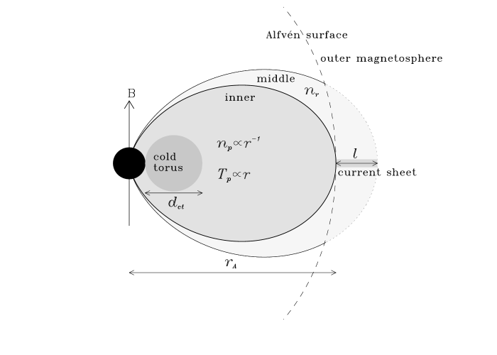
The adopted geometry is shown in Fig. 2. The layer where relativistic electrons propagate is delimited by two magnetic lines: the first is the largest closed line at a tangent to the Alfvén surface in the plane of the magnetic equator and the latter is defined by the length of the current sheets where electrons are efficiently accelerated. In each point of this shell, the “middle” magnetosphere in analogy with André et al. (a_etal88 (1988)), it is assumed that emitting electrons have a power law energy spectrum, isotropic pitch angle distribution and homogeneous spatial distribution due to magnetic mirroring.
Following the magnetically confined wind shock (MCWS) model by Babel & Montmerle (bm97 (1997)), the “inner” magnetosphere (“dead zone”) is filled by a trapped thermal plasma heated to a temperature higher then the photospheric value ( K, Kuschnig et al. k_etal99 (1999)). This hot thermal plasma progressively pushes the shock front to high magnetic latitudes, until its thermal pressure equals the wind ram pressure.
The net effect of this mechanism is the filling of the inner magnetosphere with hot thermal plasma. If the magnetosphere rotates, the density decreases linearly outward, while the temperature increases linearly (Babel & Montmerle, bm97 (1997)).
To balance the continuous supply of hot matter from the polar regions, a cool plasma down-flow is expected from the inner magnetosphere toward the stellar surface. This process causes the accumulation of cold dense material, which has been assumed for simplicity as a homogeneous torus with a circular cross-section surrounding the star (Babel & Montmerle bm97 (1997); Smith & Groote sg01 (2001)).
4.2 The parameters
In Table 2 we list the assumed stellar parameters. The dependence of our simulations on the polar magnetic field , inclination and obliquity that are not known with great accuracy will be discussed later in Sect. 5.2.
The free parameters of the model are:
-
average radius of the Alfvén surface in R∗ units;
-
thickness of the middle-magnetosphere at in R∗ units;
-
total number density of non-thermal electrons;
-
spectral index of non-thermal electron energy distribution;
-
temperature, at the stellar surface, of the thermal plasma trapped in the inner-magnetosphere;
-
electron number density, at the stellar surface, of thermal plasma;
-
cross-sectional diameter of the cold torus surrounding the star;
-
temperature of the cold torus;
-
electron number density of the cold torus.
The range of values and the assumed simulation steps of these free parameters are reported in Table 3.
In TLU04 the Alfvén surface has been located numerically by solving the equation of balance between kinetic and magnetic energy density. In this work is assumed as a free parameter, since the wind parameters of CU Vir are still unknown. The mass loss rate , assumed flowing from the whole stellar surface, and the plasma density of the wind at the Alfvén surface are thus derived as output parameters for a given and wind velocity .
For a detailed discussion of the computational method we refer to TLU04.
4.3 Numerical simulations
Since the computation is quite time consuming, we split the analysis in two steps.
4.3.1 Step 1: fitting the 8.4 GHz light curve
In this first step we can neglect the presence of the cold torus. As pointed out by TLU04, it does not have an appreciable effect in the low frequency radio emission (5 and 8.4 GHz) that arises from external magnetospheric regions, and we exclude a priori its effect in the simulations at 8.4 GHz, reducing the number of free parameters (Table 3 - step 1).
For the choice of the sampling length of the three dimensional grid we adopt the same criteria as in TLU04, with a narrow spacing (0.08 R∗) for the distance from the star center of less than 2.3 R∗, middle spacing (0.3 R∗) between 2.3 and 7 R∗, and rough spacing (1 R∗) greater than 7 R∗.
We compute the radio emission for the Stokes and at the phases that characterize the observed light curve at 8.4 GHz (see Sect. 3). The match between simulations and observations defines the possible configurations of the magnetosphere.
4.3.2 Step 2: fitting the spectra
For any set of parameters modeling the observed Stokes and at 8.4 GHz we compute the radio emission at 5 and 15 GHz to search for the ones fitting the whole observed spectra and their polarization degree.
However we cannot rule out the importance of the cold torus on the stellar emission at the frequency of 15 GHz. The free parameters that characterize the cold torus and the adopted ranges are reported in Table 3 - step 2.
| Symbols | Solutions | Units | |
|---|---|---|---|
| 12 – 17 | [R∗] | ||
| 2 | |||
| 5 | [R∗] | ||
| 0.05 – 0.2 | |||
| 0.88 – 3.54 | [ cm-3] | ||

5 Results
5.1 Prediction of the simulations
Comparison between the observations and simulations allow us to find the combinations of the model free parameters that can account for the observational behavior. The convergence of these quantities gives important informations about the physics of the external regions of this star.
The solutions derived from our analysis are reported in Table 4; the corresponding observed and computed flux light curves are plotted in Fig. 3.
The free parameters and are determined with an uncertainty smaller than the simulation steps. We find acceptable solutions for in the range 12 – 17 R∗, in 0.05 – 0.2 and in 0.88 – 3.54 cm-3. We note that the relation holds (Table 4). An important conclusion can be drawn: the column density of the relativistic electrons at the Alfvén radius is univocally determined by . For the different values of the Alfvén radius deduced from our simulations the column density is in the range cm-2.
Regarding the physical properties of the thermal plasma trapped in the inner magnetosphere, we found that the values of the electron number density and temperature that account for the observed spectral index are related as
| (1) |
while for the plasma in the cold torus
In terms of free-free
absorption coefficients (Dulk d85 (1985)),
The above relations imply that the plasma surrounding the star is almost opaque at 15 GHz, and that the cold torus around the star is completely opaque at the same frequency.
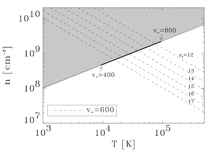
The Alfvén radius is a free parameter of our model. It is defined as the point where the magnetic energy density is equal to the kinetic energy density. If the flowing wind has terminal velocity and density , with proton mass , then:
For a given , we obtain the corresponding magnetic field strength , and consequently the thermal plasma density of the wind at the Alfvén surface. In Table 5 we list the resulting values for as a function of assuming three different values of the wind velocity (, 600 and 800 km s-1).
The mass loss rate for a spherically symmetric wind is easily computed from the continuity equation
In the presence of a magnetic dipole, only the wind flowing out from the polar caps can escape from the star and the actual mass loss rate is a fraction of , defined as the ratio of the area of the polar caps to the whole stellar surface (see TLU04). The results for and are shown in Table 5.
| a) km s-1 | |||||
|---|---|---|---|---|---|
| [R∗] | [M☉ yr-1] | [M☉ yr-1] | [ cm-3] | [K] | [cm-3] |
| 12 | 3.90 | ||||
| 13 | 2.09 | ||||
| 14 | 1.17 | ||||
| 15 | 0.68 | ||||
| 16 | 0.41 | ||||
| 17 | 0.25 | ||||
| b) km s-1 | |||||
| [R∗] | [M☉ yr-1] | [M☉ yr-1] | [ cm-3] | [K] | [cm-3] |
| 12 | 3.70 | ||||
| 13 | 2.04 | ||||
| 14 | 1.17 | ||||
| 15 | 0.69 | ||||
| 16 | 0.42 | ||||
| 17 | 0.27 | ||||
| c) km s-1 | |||||
| [R∗] | [M☉ yr-1] | [M☉ yr-1] | [ cm-3] | [K] | [cm-3] |
| 12 | 2.91 | ||||
| 13 | 1.62 | ||||
| 14 | 0.94 | ||||
| 15 | 0.56 | ||||
| 16 | 0.35 | ||||
| 17 | 0.22 | ||||
We rejected all the solutions that do not satisfy the condition of equality between the thermal plasma energy density and the wind ram pressure in the equatorial region of the Alfvén surface.
As previously discussed, the filling of the inner magnetosphere by thermal plasma is a consequence of the radiatively driven stellar wind, which accumulates material until a steady state, along lines of force of the magnetic field, is established, i.e. the thermal plasma pressure balances the wind ram pressure . This condition at the Alfvén point can be written as:
or
| (2) |
The stellar rotation implies and , hence is constant inside the inner magnetosphere, whereas the is defined by the wind velocity and wind density at (Babel & Montermle bm97 (1997)). Combining Eq. 2 and Eq. 1, we can derive the temperature and density of the thermal plasma trapped in the inner magnetosphere. The so-derived values of and are reported in Table 5 (last two columns).
In Fig. 4, the shaded area represents the pairs of and for which the thermal plasma is optically thick at 15 GHz (cold torus), while the Eq. 1 and Eq. 2, for different values of , are represented by the continuous and dashed line respectively. The intersection, marked with a thick segment, defines the ranges of values of and that satisfy the equality condition and correctly reproduce the observed radio light curves.
5.2 Dependence on the stellar parameters
Since the distance and stellar radius of Cu Vir are known with good accuracy, the major uncertainty on the assumed parameters is related to the magnetic field strength and geometry. In particular, the value of reported in the literature ranges from 2200 to 3800 Gauss (Landstreet et al. 1977; TLL00). We thus examined whether our choice of =3000 Gauss significantly influences the model results. We verified that a variation of 25% in results in a variation of 25% in , while the other parameters remain unaffected.
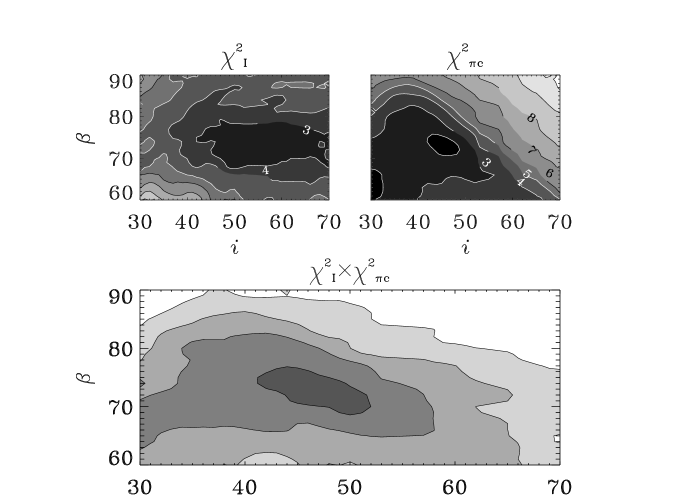
Moreover, we tested the sensitivity of the model to values of inclination of the rotation axis () and obliquity of the magnetic axis () different from those adopted in our calculations. We minimize the normalized function for the light curves (total flux density and the fraction of circular polarization) at 8.4 GHz. To restrict the computational time, we limit this analysis to the set of model parameters associated with the lowest value of the Alfvén radius ( R∗). The maps of are displayed in Fig. 5 (top panels). Dark areas correspond to pairs of and with lower , for which we find the best match between simulations and observations. We note that the from the total flux fit is not well correlated to the relative to the fit of the circular polarization. The product of these two matrices, Fig. 5 (bottom panel), gives the combination of and that better reproduces both total flux and circular polarization. We note that the most probable values of and are restricted in a well defined range of values, respectively: and . We note that the values of and from the literature are well inside the previous intervals.
5.3 Limits of the model
While the modulation of the total flux density light curve observed at 5 GHz is well reproduced by our simulations, we are not able to match the two peaks observed close to the phases 0.40 and 0.85 of the circularly polarized flux light curve. These are also the phases of the coherent emission observed at 1.4 GHz (Fig. 1, bottom panel), a coincidence suggesting that the two peaks are residuals of the Electron Cyclotron Maser Emission (ECME) mechanism (TLL00). As the ECME mechanism is not considered in our model, which computes only incoherent gyrosynchrotron, it cannot reproduce these observed peaks.
At 15 GHz, a stronger and broader polarization is expected in the range 0.9 – 1.3 (Fig. 3). This discrepancy could be ascribed to the simple dipolar configuration adopted for the magnetic field. In the magnetospheric regions close to the star, where the bulk of 15 GHz radiation is emitted, the high order components of the magnetic field of CU Vir (Hatzes h97 (1997); Kushinig et al. k_etal99 (1999); TLL00; Glagolevskij & Gerth gg02 (2002)) cannot be neglected. A simple dipole provides a symmetric total flux light curve and an enhancement of the fraction of polarization when the line of sight is close to the magnetic pole, where the magnetic lines are almost parallel. In the presence of multipolar components the radio flux light curves would not be symmetric and the fraction of the polarization would be reduced.
6 Discussion
In the following we will analyze physical information about the stellar magnetosphere that can be inferred from the results of our simulations.
6.1 The acceleration process
The convergence of the value of the spectral index of the emitting electron distribution () toward indicates that the acceleration process occurs in the current sheets just outside the Alfvén radius. This value agrees with the one derived in the case of solar flares by Zharkova & Gordovskyy (zg05 (2005)), who found a spectral index for the non-thermal electrons accelerated in the neutral reconnecting current sheets of solar magnetic loops. In addition, from the ratio between (Table 4) and the density of the electrons of the wind at the Alfvén point (Table 5), we can estimate that the efficiency of the acceleration process for non-thermal electrons is . The efficency inferred by our analysis is consistent with the acceleration efficiency in large stationary unstable current sheets associated with coronal loops during solar flares (Vlahos et al. v_etal04 (2004)).
6.2 The radio emitting region
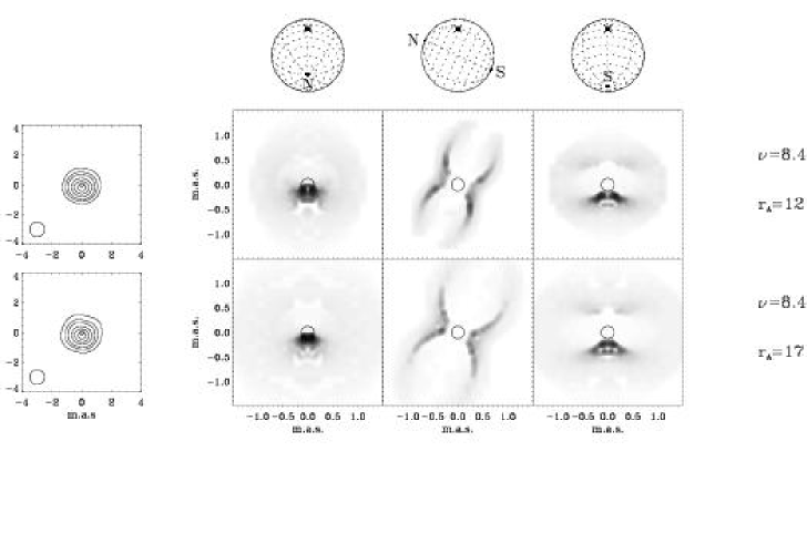
We investigated the possibility of discrimining among the previous possible values of the Alfvén radius by using high angular resolution radio observations in the future. In Fig. 6 the brightness spatial distributions at 8.4 GHz obtained for the extreme values of (respectively 12 and 17 ) are shown. The simulated radio maps have been calculated for three rotational phases: the stellar orientations that show the north and south poles, associated with the two maxima and the orientation that gives a null effective magnetic field, associated with the minimum of the radio light curve. In the right panel of Fig. 6, the different extension of the radio source for the two cases analyzed is clearly visible. However such a difference is not so obvious when looking at the radio emission arising from regions near the stellar surface, where the highest fraction of the magnetospheric radio emission originates.
For the Very Long Baseline Interferometry (VLBI) technique, that can be used to map CU Vir at milli arcsecond scales, we derived two “synthetic” maps at VLBI resolution, shown on the left side of Fig. 6, obtained as the average of hypothetical 8 hours observation around the stellar phase coinciding with the null effective magnetic field, convolved with a Gaussian 1 mas beam. It is clear that the present capability of VLBI observations does not allow us to discriminate between the extreme values of the Alfvén radius of CU Vir predicted by our model.
6.3 The thermal plasma
The physical condition in the inner magnetosphere play an important role in the emerging radio flux because of the free-free absorption by the plasma, which affects the modulation of the radio light curves and the spectrum of the source. The comparison between our model prediction and multifrequency observations reveals the presence of a torus of material colder and denser than the trapped thermal plasma. This is necessary to reproduce the correct scale of the total flux density in the 15 GHz light curve of CU Vir. The electron number density () and temperature () of the plasma of the cold torus, are within the shaded area of the plane shown in Fig. 4, where the optical depth of the cold torus is higher than 1 at 15 GHz. Higher frequency measurements (for example 22 and 43 GHz) could characterize the spatial distribution of the thermal plasma in the deep magnetospheric regions, near the stellar surface.
The temperature and density of the thermal plasma trapped in the inner magnetosphere are assigned for a given Alfvén radius and wind velocity (Table 5). As a by-product of our analysis, we estimate the X-ray emission from the thermal plasma trapped in the stellar inner magnetosphere of CU Vir as a function of and . Following the same procedure described in TLU04, for each element of the 3D cubic grid that samples the magnetosphere, we computed the thermal bremsstrahlung emission coefficients and the emerging power integrated between 0.1 and 10 keV, in the typical energy range of X-ray telescopes like Chandra and XMM. The resulting X-ray fluxes at the Earth are displayed in Fig. 7.
The stellar X-ray emission is a function of the size of the Alfvén surface (Fig. 7) and, in particular, it decreases as the Alfvén radius increases. This is a consequence of the lower temperature and density of the plasma in the inner magnetosphere for increasing . For the same reason, lower wind velocities cause a lower X-ray emission.
On the basis of the values derived from our calculations, we conclude that the X-ray emission from CU Vir is below the detection limit of the ROSAT all sky survey (the average background at the position of CU Vir in the RASS is higher than erg cm-2 s-1). Nevertheless, for exposure times of a few tens of kilo-seconds, Chandra and XMM can reach an X-ray detection limit close to erg cm-2 s-1, which is lower than the X-ray fluxes predicted from several model solutions.
Within our model, measurement of the X-ray flux of CU Vir could place an important constraint on the physical condition in the magnetosphere.

7 Conclusion
The radio magnetosphere of CU Vir has been extensively studied using of the first multifrequency VLA observations, covering the entire rotational period, for both the total flux density (Stokes ) and the circular polarization (Stokes ). We have successfully modeled the observed flux modulation and the circular polarization light curves using the 3D model developed by us (TLU04), modified to resolve the circular polarization intensity.
We pointed out the importance of multi-frequency and dual polarization observations throughout the rotational period to gain insight into the physical conditions of the circumstellar environments surrounding MCP stars.
Our results are:
- -
-
-
The size of the CU Vir inner magnetosphere has been constrained in the range: R∗;
-
-
we evaluated the mass loss rate of CU Vir, which up to now was not determined for this star, to be about M☉ yr-1;
-
-
the temperature of the thermal electrons trapped in the inner magnetosphere can reach K and can give detectable X-ray emission;
-
-
the presence of an accumulation of cold and dense material around the star has been shown and limits for its size and physical conditions (temperature and density) are given;
-
-
the acceleration in the current sheets produces a non-thermal electron population with a hard energetic spectrum ( with ), and the acceleration process has an efficiency of about .
The limits of our model to reproduce all the observed features, for example the two peaks at phases and observed in the 5 GHz light curve for the circular polarization and the shape of the light curves at 15 GHz, have been interpreted respectively as due to the residual of the ECME mechanism (responsible for the features previously observed at 1.4 GHz, TLL00) and as evidence of a multipolar component in the magnetic field of CU Vir.
Acknowledgements.
We thank the referee for his/her constructive criticism which enabled us to improve this paper.References
- (1) André, P., Montermle, T., Feigelson, E.D., Stine, P.C., Klein, K.L. 1988, ApJ, 335, 940
- (2) Babcock, H.W. 1949, Observatory, 69, 191
- (3) Babel, J. 1996, A&A, 309, 867
- (4) Babel, J., Montermle, T. 1997, A&A, 323, 121
- (5) Borra, E.F., Landstreet, J.D. 1980, ApJS, 42, 421
- (6) Drake, S.A., Abbot, D.C., Bastian, T.S., Bieging, J.H., Churchwell, E., Dulk, G., Linsky, J.L. 1987, ApJ, 322, 902
- (7) Dulk, G.A. 1985, ARA&A, 23, 169
- (8) European Space Agency 1997, Hypparcos Catalogue SP-1200
- (9) Glagolevskij, Y.V., Gerth, E. 2002, A&A, 382, 935
- (10) Havnes, O., Goertz, C.K. 1984, A&A, 138, 421
- (11) Hatzes, A.P. 1997, MNRAS, 288, 153
- (12) Hunger, K., Groote, D. 1999, A&A, 351, 554
- (13) Klein, K.L., Trotter, G. 1984, A&A, 141, 67
- (14) Kuschnig, R., Ryabchikova, T.A., Piskunov, N.E., Weiss, W.W., Gelbmann, M.J. 1999, A&A, 348, 924
- (15) Landstreet, J.D., Borra, E.F. 1977, ApJL, 212, 43
- (16) Landstreet, J.D. 1990, ApJ, 352, 5
- (17) Leone, F. 1991, A&A, 252, 198
- (18) Leone, F., Umana, G. 1993, A&A, 268, 667
- (19) Leone, F., Trigilio, C., Umana, G. 1994, A&A, 283, 908
- (20) Lim, J., Drake, S.A., Linsky, J.L. 1996, ASPC, 93, 324
- (21) Linsky, J.L., Drake, S.A., Bastian, T.S. 1992, ApJ, 393, 341
- (22) Mathys, G. 1991, A&AS, 89, 121
- (23) North, P. 1998, A&A, 334, 181
- (24) Pyper, D.M., Ryabchikova, T., Malanushenko, V., Kuschnig, R., Plachinda, S., Savanov, I. 1998, A&A, 339, 822
- (25) Ramaty, R. 1969, ApJ, 158, 753
- (26) Shore, S.N. 1987, AJ, 94, 731
- (27) Shore, S.N., Brown, D.N., Sonneborn, G. 1987, AJ, 94, 737
- (28) Shore, S.N., Brown, D.N. 1990, ApJ, 365, 665
- (29) Smith, M.A., Groote, D. 2001, A&A, 372, 208
- (30) Stibbs, D.W.N. 1950, MNRAS, 110, 395
- (31) Trigilio, C., Leto, P., Leone, F., Umana, G., Buemi, C. 2000, A&A, 362, 281 (TLL00)
- (32) Trigilio, C., Leto, P., Umana, G., Leone, F., Buemi, C.S. 2004, A&A, 418, 593 (TLU04)
- (33) Usov, V.V., Melrose, D.B. 1992, ApJ, 395, 575
- (34) Vlahos, L., Isliker, H., Lepreti, F. 2004, ApJ, 608, 540
- (35) Zharkova, V.V., Gordovskyy, M. 2005, MNRAS, 356, 1107
Appendix A Calculation of circular polarization
The circularly polarized intensity may be obtained using the relation, given by Ramaty (r69 (1969)):
| (3) |
where are solutions of the radiative transfer equation for the ordinary (sign “”) and extraordinary (sign “”) modes (Klein & Trotter kt84 (1984)):
| (4) |
with and gyrosynchrotron emission and absorption coefficients, and refractive index and polarization coefficient for the two modes respectively. is the angle between the wave vector and the group velocity, given by the equation:
with the angle between the wave vector and the magnetic field. The equation 4 was numerically solved, along a path parallel to the line of sight, using the method developed by us in TLU04.
In accordance with classical physics, for propagation parallel to the magnetic field lines ( and ), the ordinary mode is characterized by the electric field vector rotating in the sense of the electrons, counterclockwise in the case of a wave approaching the observer, therefore the polarization sense for the ordinary mode is LCP; conversely the extraordinary mode has a polarization sense RCP.
VLA measurements of the wave circular polarization state are in accordance with the IAU and IEEE orientation/sign convention, unlike the classical physics usage. Therefore to compare our simulations with the VLA observations we have to change the sign of the result of equation 3.