Collision of two identical hypersonic stellar winds in binary systems

Abstract

We investigate the hydrodynamics of two identical hypersonic stellar winds in a binary system. The interaction of these winds manifests itself in the form of two shocks and a contact surface between them. We neglect the binary rotation and assume that the gas flow ahead of the shocks is spherically symmetrical. In this case the contact surface that separates the gas emanated from the different stars coincides with the midplane of the binary components. In the shock the gas is heated and flows away nearly along the contact surface. We find the shock shape and the hot gas parameters in the shock layer between the shock and the contact surface.

1 Introduction

Stars of various types drive stellar winds with widely differing characteristics. In binary systems that consist of such stars the winds flowing out of the stars may strike each other. Collision of stellar winds may result in an observational appearance if the winds are rather powerful. Among all stars, massive OB and Wolf-Rayet (WR) stars have the strongest winds. The mass-loss rate $\dot{M}$ is as high as $\sim 10^{-6}-10^{-5}\,M_{\odot}{\rm yr}^{-1}$ for O and B stars or even higher ($\sim 10^{-5}-10^{-4}\,M_{\odot}{\rm yr}^{-1}$) for WR stars. The terminal velocity of the matter outflow is $V^{\infty}\sim(1-5)\times 10^{3}$ km s^-1 for OB and WR stars. The kinetic energy carried away by the winds is $\sim 10^{35}-10^{38}$ ergs s^-1. In the region where the two winds collide some part of this energy may be transformed to other forms of energy (for example, the thermal energy of hot gas or the energy of ultra-relativistic electrons), and then, radiated at different frequencies. At present a variety of phenomena related to the collision of the stellar winds are observed for WR+OB and OB+OB binaries (for a review, see Williams 1999; Cherepashchuk 2000; Corcoran et al. 2005). In particular, it is found that the X-ray luminosities of massive binaries are significantly higher (by a factor of $\sim 10^{2}$ for some systems) than the total X-ray luminosities of their single counterparts in a statistical sense (Pollock 1987; Chlebowski & Garmany 1991). The analysis of the energy spectra and the time variability of the X-ray emission indicates that the X-ray excess is emitted from the region where the two winds collide (Moffat et al. 1982; Chlebowski 1989; Williams et al. 1990; Corcoran et al. 1996; Corcoran 2003). The observational data on the X-ray emission from massive binaries are well consistent with the model where strong shocks form because of the wind-wind collision (Prilutskii and Usov 1975, 1976; Cherepashchuk 1976; Usov 1990, 1992, 1995; Stevens, Blondin, & Pollock 1992; Antokhin, Owocki, & Brown 2004). In this model the outflowing gas is heated behind of the shocks to temperatures of $\sim 10^{6}-10^{7}$ K and radiate X-ray emission that is observed as the X-ray excess. Besides, the shock waves in massive binaries are able to accelerate electrons to ultrarelativistic energies, and these electrons can generate non-thermal radio emission via the synchrotron mechanism in the vicinity of the shocks (Williams et al. 1990; Eichler & Usov 1993; Williams, van der Hucht, & Spoelstra 1994; White & Becker 1995; Dougherty et al. 1996; Jardine, Allen, & Pollock 1996; Chapman et al. 1999; Setia Gunawan et al. 2000; Monnier et al. 2002; Pittard et al. 2006). For several nearby WR+OB binaries (WR140, WR146 and WR147), the radio sources are spatially resolved, and the radio emission model based on the wind-wind collision is confirmed (Moran et. al. 1989; Churchwell et al. 1992; Niemela et al. 1998; Dougherty, Williams, & Pollacco 2000) Dust formation may also occur in the wind collision region (Usov 1991) and is observed for several massive binaries as an IR excess (Williams & van der Hucht 1992; Marchenko, Moffat, & Grosdidier 1999; Monnier, Tuthill, & Danchi 2002; Williams et al. 2003).

The hydrodynamics of colliding winds has been studied both analytically (Galeev, Pilyugin, & Usov 1989; Bairamov, Pilyugin, & Usov 1990; Usov 1992, 1995) and numerically (Luo, McCray, & Mac Low 1990; Myasnikov & Zhekov 1991; Stevens, Blondin, & Pollock 1992; Pittard & Stevens 1997; Zhekov & Skinner 2000; Henley, Stevens, & Pittard 2003). In the analytical studies it was assumed that the wind of star 1 (the primary) is much stronger than that of star 2 (the secondary). In this case the wind-wind collision zone is near the secondary on the side facing the primary, and its characteristic size is much smaller than the distance between the components of the binary. The undisturbed gas stream from star 1 ahead of the shock was considered as plane-parallel. The wind from star 2 was assumed to be spherically symmetrical. It is a reasonable approximation, for instance, to the WR+OB binaries where the wind momentum of the OB star is $\sim 10-10^{3}$ times smaller than that of the WR star, i.e., $\eta=\dot{M}_{\rm OB}V_{\rm OB}^{\infty}/\dot{M}_{\rm WR}V_{\rm WR}^{\infty}\sim 10^{-3}-10^{-1}\ll 1$. However, this approximation is too rough for binaries with nearly the same stellar winds ($\eta\sim 1$). In this paper we consider the wind-wind collision in the case when the colliding winds are identical in strength ($\eta=1$).

The paper is organized as follows. In § 2 we discuss the properties of the undisturbed gas that flows away from the star vicinity. In § 3 we formulate the problem of collision of two identical hypersonic steady winds in a binary system and outline both the hydrodynamic equations, which describe the motion of the hot gas behind the shock, and boundary conditions on them. In § 4 we solve the set of hydrodynamic equations and boundary conditions and find the structure of the shock and the parameters of the hot gas in the shock layer. Finally, in § 5 we discuss our results and some potential astrophysical applications.

2 Formulation of the problem

We consider the hydrodynamics of two identical hypersonic steady winds in a binary system. We assume that the gas flow from the binary components is spherically symmetrical, nonviscous and nonheat conductive. The energy losses of the gas by radiation are neglected, i.e., the gas flow is adiabatic. We also neglect the rotation of the binary and its components.

The interaction of two colliding stellar winds will manifest itself in the form of two shocks separated by a contact surface (see Fig. 1). The winds from the binary components flow radially out to the shocks. In the shock the gas is heated to the postshock temperature of $\sim 10^{7}V_{8}$ K, where $V_{8}$ is the preshock wind velocity perpendicular to the shock in units of $10^{8}$ cm s^-1. Behind the shock the hot gas flows away from the binary system nearly along the contact surface (e.g., Usov 1992 and below). The contact surface separates the hot gas that has been emanated from the different components. For an arbitrary value of $\eta$ the contact surface has a rather complex shape (e.g., Canto et al. 2006). In our case of two equal winds ($\eta=1$), there is a reflection symmetry about the midplane of the two stars, and the contact surface coincides with the midplane (see Fig. 1).

2.1 Basic equations

We start from the set of equations, which describes the gas flow in our approximation,

$${\rm div}\,(\rho{\bf V})=0\,,$$ (1)

$$\rho({\bf V}{\bf\nabla}){\bf V}=-{\bf\nabla}p\,,$$ (2)

$$\rho{\bf V}{\bf\nabla}(H+|{\bf V}|^{2}/2)=0\,,$$ (3)

where ${\bf V}$ is the velocity of the gas, $\rho$ is its density, $p$ is the total pressure,

$$H={\gamma\over{\gamma-1}}{p\over\rho}$$ (4)

is the specific enthalpy, $T$ is the temperature, and $\gamma$ is the ratio of heat capacities at constant pressure and at constant volume (e.g., Chernyi 1961). Equation (1) gives conservation of mass, while equations (2) and (3) conserve the momentum and total energy, respectively.

In the shock layers between the shocks and the contact surface the hot gas may be considered as a rarefied totally ionized plasma. For such a plasma, we have

$$p=(N_{e}+N_{i})kT={\rho kT\over m_{p}\mu}\,,$$ (5)

$$N_{i}={\rho\over m_{p}A}\,,\,\,\,\,\,N_{e}=N_{i}Z\,,\,\,\,\,\,{\rm and}\,\,\,\,\,\gamma={5\over 3}\,,$$ (6)

where $N_{e}$ is the density of electrons, $N_{i}$ is the density of ions, $k$ is the Boltzmann constant, $A$ is the atomic weight of ion, $Z$ is its electrical charge, $\mu=A/(1+Z)$ is the mean molecular weight, and $m_{p}$ is the proton mass.

2.2 Boundary conditions

The gas parameters ahead of the shock (index 1) and behind the shock (index 2) are related via the Rankine-Hugoniot relations

$$\rho_{1}V^{(n)}_{1}=\rho_{2}V^{(n)}_{2},\,\,\,p_{1}+\rho_{1}[V^{(n)}_{1}]^{2}=p_{2}+\rho_{2}[V_{2}^{(n)}]^{2},$$

$$V_{1}^{(\tau)}=V_{2}^{(\tau)},\,\,\,\,H_{1}+{[V_{1}^{(n)}]^{2}\over 2}=H_{2}+{[V_{2}^{(n)}]^{2}\over 2}\,.\,\,\,\,$$ (7)

Indices $n$ and $\tau$ denote the normal and tangential components of the gas velocity ${\rm V}$. The condition $V^{(n)}$=0 is met on the contact surface. This condition and the Rankine-Hugoniot relations (7) are the full set of boundary conditions for the set of equations (1)-(5) needed to find the parameters of hot gas in the shock layers.

3 Stellar winds from massive stars

The luminosity of a massive star is very high, and the radiation pressure is responsible for the outflow of gas and its subsequent acceleration. The gas velocity $V(r)$ varies from almost zero at the surface of the star ($r=R)$ to some terminal value at the distance $r_{*}\simeq(3-5)R$ from the stellar center (e.g., Barlow 1982).

At $r\gtrsim r_{*}$ the gas acceleration is more or less finished, and the gravity of the star may be neglected. In this case, from equations (1)-(4) the spherically symmetric supersonic (${\mathfrak{M}}>1$) flow of gas may be described by

$$\left({r_{*}\over r}\right)^{2}=\left({{\mathfrak{M}}\over{\mathfrak{M}}_{*}}\right)\left[{(\gamma-1){\mathfrak{M}}^{2}_{*}+2\over(\gamma-1){\mathfrak{M}}^{2}+2}\right]^{\gamma+1\over 2(\gamma-1)},$$ (8)

$${V\over V_{*}}=\left({{\mathfrak{M}}\over{\mathfrak{M}}_{*}}\right)\left[{(\gamma-1){\mathfrak{M}}^{2}_{*}+2\over(\gamma-1){\mathfrak{M}}^{2}+2}\right]^{1/2},$$ (9)

$${\rho\over\rho_{*}}=\left[{(\gamma-1){\mathfrak{M}}^{2}_{*}+2\over(\gamma-1){\mathfrak{M}}^{2}+2}\right]^{1\over\gamma-1},$$ (10)

$${p\over\rho_{*}V_{*}^{2}}={1\over\gamma\,{\mathfrak{M}}^{2}_{*}}\left[{(\gamma-1){\mathfrak{M}}^{2}_{*}+2\over(\gamma-1){\mathfrak{M}}^{2}+2}\right]^{\gamma\over\gamma-1},$$ (11)

$${2H\over V_{*}^{2}}={2\over(\gamma-1)\,{\mathfrak{M}}_{*}^{2}}\left[{(\gamma-1){\mathfrak{M}}^{2}_{*}+2\over(\gamma-1){\mathfrak{M}}^{2}+2}\right]\,,$$ (12)

where ${\mathfrak{M}}=V/V_{s}$ is the Mach number and $V_{s}$ is the sound speed in the outflowing gas. The gas parameters marked by the sign _∗ are taken at $r=r_{*}$. For winds from massive stars, we have $V\sim 10^{3}$ km s^-1, $V_{s}\sim 10$ km s^-1, and ${\mathfrak{M}}\sim 10^{2}\gg 1$.

For $(\gamma-1){\mathfrak{M}}^{2}_{*}\gg 1$ equations (8)-(12) are simplified and yield

$${\mathfrak{M}}={\mathfrak{M}}_{*}\left({r\over r_{*}}\right)^{\gamma-1}\gg 1\,,$$ (13)

$$V=V_{*}=V^{\infty},\,\,\,\,\,\,\,{\rho\over\rho_{*}}=\left({r_{*}\over r}\right)^{2},$$ (14)

$${p\over\rho_{*}V_{*}^{2}}={1\over\gamma\,{\mathfrak{M}}^{2}_{*}}\left({r_{*}\over r}\right)^{2\gamma}\ll 1\,,$$ (15)

$${2H\over V_{*}^{2}}={2\over(\gamma-1)\,{\mathfrak{M}}_{*}^{2}}\left({r_{*}\over r}\right)^{2(\gamma-1)}\ll 1\,.$$ (16)

From equations (15) and (16) we can see that in a supersonic flow far from the star ($r\gtrsim r_{*}$) the effects of the thermal pressure and the thermal energy are of the order of ${\mathfrak{M}}^{-2}$ that is $\sim 10^{-4}$ or less for massive stars. In our study, we neglect these effects, and the gas flow ahead of the shocks is described by

$${\bf V}=V^{\infty}{{\bf r}\over r}\,,\,\,\,\,\,\,\,\rho=\rho_{*}\left({r_{*}\over r}\right)^{2}\,,\,\,\,\,\,p=H=0\,.$$ (17)

4 Collision of two equal winds with terminal velocities

In Section 2 it is noted that for two colliding stellar winds the gas flow has reflection symmetry about the contact surface that coincides with the midplane of the binary components (see Fig. 1). Therefore, the problem of collision of two equal winds is identical with the problem of collision of one of the winds with the midplane. The latter problem is considered in this paper. We assume that the binary is wide ($D>r_{*}$), and the terminal velocity is reached by the wind ahead of the shock, where $D$ is a half of the binary separation.

4.1 Shock layer

In the shock layer the position of a point may be defined by the two coordinates $x$ and $y$ that are the distances from the point to the binary axis and the contact plane, respectively (see Fig. 2). However, it is easier to solve the set of equations (1)-(4) using the independent variables $\psi$ and $x$, where $\psi$ is the stream function defined by the equality

$$d\psi=\rho uxdy-\rho vxdx\,,$$ (18)

where $u$ and $v$ are the velocity components in the $x$ and $y$ directions, respectively.

In the new independent variables $\psi$ and $x$ the set of equations (1)-(4) can be written as

$${\partial y\over\partial\psi}={1\over\rho ux},\;\;\;\;{\partial y\over\partial x}={v\over u}\ ,$$ (19)

$${\partial v\over\partial x}=-x{\partial p\over\partial\psi}\ ,$$ (20)

$$\rho\bigg{(}u{\partial u\over\partial x}+v{\partial v\over\partial x}\bigg{)}=-{\partial p\over\partial x}\ ,$$ (21)

$${\partial\over\partial x}\bigg{(}H+{u^{2}+v^{2}\over 2}\bigg{)}=0\,.$$ (22)

It is convenient to introduce dimensionless variables via

$$\overline{x}={x\over D}\,,\,\,\,\,\,\,\,\overline{y}={y\over D}\,,\,\,\,\,\,\,\,\overline{r}={r\over D}\,,$$

$$\overline{u}={u\over V^{\infty}}\,,\,\,\,\,\,\,\,\overline{v}={v\over V^{\infty}}\,,$$

$$\overline{p}={p\over\rho_{*}(V^{\infty})^{2}}\left({D\over r_{*}}\right)^{2},\,\,\,\,\,\,\,\overline{H}={2H\over(V^{\infty})^{2}}\,,$$

$$\overline{\rho}={\rho\over\rho_{*}}\left({D\over r_{*}}\right)^{2},\,\,\,\,\,\,\,\,\overline{\psi}={\psi\over\rho_{*}V^{\infty}r_{*}^{2}}\,.$$ (23)

In these variables equations (19)-(22) take the form:

$${\partial\overline{y}\over\partial\overline{\psi}}={1\over\overline{\rho}\,\overline{u}\,\overline{x}},\;\;\;\;{\partial\overline{y}\over\partial\overline{x}}={\overline{v}\over\overline{u}}\ ,$$ (24)

$${\partial\overline{v}\over\partial\overline{x}}=-\overline{x}{\partial\overline{p}\over\partial\overline{\psi}}\ ,$$ (25)

$$\overline{\rho}\bigg{(}\overline{u}{\partial\overline{u}\over\partial\overline{x}}+\overline{v}{\partial\overline{v}\over\partial\overline{x}}\bigg{)}=-{\partial\overline{p}\over\partial\overline{x}}\ ,$$ (26)

$${\partial\over\partial\overline{x}}\bigg{(}\overline{H}+\overline{u}^{2}+\overline{v}^{2}\bigg{)}=0\,.$$ (27)

Using the boundary conditions (7) at the shock (see Fig. 2) and equation (17) for the gas parameters near and ahead of the shock, we can get the gas parameters near and behind the shock (index $s$):

$$\overline{u}_{s}=\epsilon\,\cos\alpha\,\sin(\alpha+\varphi)-\cos(\alpha+\varphi)\,\sin\alpha\,,$$ (28)

$$\overline{v}_{s}=-[\epsilon\,\sin\alpha\,\sin(\alpha+\varphi)+\cos(\alpha+\varphi)\,\cos\alpha]\,,$$ (29)

$$\overline{p}_{s}={1\over\overline{r}_{s}^{2}}(1-\epsilon)\,\sin^{2}(\alpha+\varphi)\,,$$ (30)

$$\overline{H}_{s}=(1-\epsilon^{2})\,\sin^{2}(\alpha+\varphi)\,,$$ (31)

where $\epsilon$ is the ratio of the gas density ahead of the shock to that behind it,

$$\epsilon={\gamma-1\over\gamma+1}\,,$$ (32)

$\alpha$ is the angle between the tangent to the shock wave and the binary axis, $\varphi$ is the angle between the radius-vector ${\bf r}$ from the center of the star and the binary axis, and

$$\overline{r}_{s}=[\overline{x}^{2}+(1-\overline{y}_{s})^{2}]^{1/2}$$ (33)

is the dimensionless distance from the stellar center to the shock wave (see Fig. 2). For $\gamma={5\over 3}$, we have $\epsilon={1\over 4}$.

The equation of the shock shape

$$\overline{y}=\overline{y}_{s}(x)$$ (34)

is connected with the angle $\alpha$ by

$$\overline{y}_{s}^{\prime}\equiv{d\overline{y}_{s}\over d\overline{x}}=\tan^{-1}\alpha\,.$$ (35)

From equations (17) and (18) the stream function at the shock wave may be written as

$$\overline{\psi}_{s}={\int_{0}^{\overline{x}}}{\sin\,(\alpha+\varphi)\,\overline{x}d\overline{x}\over\overline{r}^{2}_{s}}\,.$$ (36)

In the dimensionless coordinates $\overline{x}$ and $\overline{\psi}$ the equation of shock shape is $\overline{\psi}=\overline{\psi}_{s}(\overline{x})$.

Using equations (33) and (35), equation (36) can be rewritten as

$$\overline{\psi}_{s}={\int_{0}^{\overline{x}}}{(1+\overline{x}\,\overline{y}^{\prime}_{s}-\overline{y}_{s})\,\overline{x}d\overline{x}\over[1+(\overline{y}^{\prime}_{s})^{2}]^{1/2}[\overline{x}^{2}+(1-\overline{y}_{s})^{2}]^{3/2}}\,.$$ (37)

Near the contact plane the velocity component perpendicular to this plane is zero, i.e.,

$$\overline{v}=0\,\,\,\,\,\,\,{\rm at}\,\,\,\overline{y}=0\,.$$ (38)

To find the shock shape (34) and the parameters of the hot gas in the shock layer we solve the set of equations (4) and (24)-(27) with the boundary conditions (28)-(31) and (38) by the method of Chernyi (1961) in which $\epsilon$ is considered as a small parameter. Henceforth, we omit the bars over the dimensionless variables.

We seek a solution of equations (24)-(27) in the form of a series in powers of $\epsilon$ in the following form:

$$y=\epsilon y_{0}\,,\,\,\,\,\,u^{2}=u_{0}^{2}+\epsilon u_{1}^{2}\,,\,\,\,\,\,v=\epsilon v_{0}\,,$$ (39)

$$p=p_{0}+\epsilon p_{1}\,,\,\,\,\,\rho={\rho_{0}\over\epsilon}+\rho_{1}\,,\,\,\,\,H=H_{0}+\epsilon H_{1}\,.$$ (40)

Substituting these series into equations (4) and (24)-(27) and equating the terms with the same power of $\epsilon$, we obtain the following equations for determining the terms of the series:

$${\partial u_{0}\over\partial x}=0\,,\,\,\,\,\,\,{\partial p_{0}\over\partial\psi}=0\,,\,\,\,\,\,\,{\partial H_{0}\over\partial x}=0\,,$$ (41)

$$v_{0}=u_{0}{\partial y_{0}\over\partial x}\,,\,\,\,\,\,\,{\partial y_{0}\over\partial\psi}={1\over\rho_{0}x(u_{0}^{2}+\epsilon u_{1}^{2})^{1/2}}\,,$$ (42)

$$H_{0}={2\gamma\over(\gamma+1)}{p_{0}\over\rho_{0}}\,,\,\,\,\,\,\,H_{1}=H_{0}\left({p_{1}\over p_{0}}-{\rho_{1}\over\rho_{0}}\right)\,,$$ (43)

$${\partial v_{0}\over\partial x}=-x{\partial p_{1}\over\partial\psi}\,,\,\,\,\,\,\,{\rho_{0}\over 2}{\partial u_{1}^{2}\over\partial x}=-{\partial p_{0}\over\partial x}\,.$$ (44)

$${\partial\over\partial x}(H_{1}+u_{1}^{2})=0\,.$$ (45)

We keep the first order term ($\epsilon u_{1}^{2}$) in the second equation of (42) derived in zero approximation over $\epsilon$. We do this because it has been shown that in this case the analytical results on the shock layer structure are more consistent with the results of numerical simulations (see Hayes & Probstein 1959; Lunev 1975 and below).

Equations (41) and (45) are integrable by quadrature:

$$u_{0}=u_{0}(\psi)\,,\,\,\,\,\,\,\,p_{0}=p_{0}(x)\,,$$ (46)

$$H_{0}=H_{0}(\psi)\,,\,\,\,\,\,\,\,\rho_{0}={2\gamma\over(\gamma+1)}\,{p_{0}(x)\over H_{0}(\psi)}\,,$$ (47)

$$u_{1}^{2}=-2\int_{0}^{x}{dp_{0}(x)\over dx}{dx\over\rho_{0}(x,\psi)}+u^{2}_{*}(\psi)\,,$$ (48)

$$y_{0}={1\over x}\int_{0}^{\psi}{d\psi\over\rho_{0}(x,\psi)[u_{0}^{2}(\psi)+\epsilon u_{1}^{2}(x,\psi)]^{1/2}}+y_{*}(x)\,,$$ (49)

$$v_{0}=u_{0}(\psi){\partial y_{0}(x,\psi)\over\partial x}\,,$$ (50)

$$p_{1}=-\int_{0}^{\psi}{\partial v_{0}(x,\psi)\over\partial x}\,{d\psi\over x}+p_{*}(x)\,,$$ (51)

$$H_{1}=-u_{1}^{2}(x,\psi)+H_{*}(\psi)\,,$$ (52)

$$\rho_{1}=\rho_{0}(x,\psi)\left[{p_{1}(x,\psi)\over p_{0}(x)}-{H_{1}(x,\psi)\over H_{0}(\psi)}\right]$$ (53)

where $u_{0}(\psi)$, $p_{0}(x)$, $H_{0}(\psi)$, $u_{*}(\psi)$, $y_{*}(x)$, $p_{*}(x)$, and $H_{*}(\psi)$ are arbitrary functions that can be determined from the boundary conditions at the shock wave and at the contact surface.

Since $y=0$ and $\psi=0$ at the contact surface, from equation (49) we have $y_{*}(x)=0$.

4.1.1 Zero approximation

In the series (39) and (40) we keep only the first terms marked by 0 (zero approximation). To find the values $u_{0}$, $p_{0}$, $H_{0}$, and $\psi_{0,s}$ in this approximation we can take that the shock wave coincides with the contact plane, and $\alpha$ is equal to $\pi/2$. From equations (28), (30), and (31) we have the following boundary conditions:

$$u_{0,s}=\sin\varphi\,,\,\,\,\,p_{0,s}={\cos^{2}\varphi\over r_{s}^{2}}\,,\,\,\,\,H_{0,s}=\cos^{2}\varphi\,.$$ (54)

From equation (37), we obtain

$$\psi_{0,s}=\int_{0}^{x}{xdx\over(1+x^{2})^{3/2}}=1-{1\over(1+x^{2})^{1/2}}\,.$$ (55)

Below, instead of $\psi$ we use the new coordinate $t$ which is the length along the shock wave, measured from the binary axis to the point where the stream line $\psi$ intersects the shock (see Fig. 2).

At the shock wave the value of $t$ in the zero approximation is equal to $x$, and substituting $t$ for $x$ into equation (55) we have the following connection between $\psi_{0}$ and $t$:

$$\psi_{0}=1-{1\over(1+t^{2})^{1/2}}\,.$$ (56)

In the new independent variables $t$ and $x$ ($0\leq t\leq x$), equations (46), (47), and (54) yield

$$u_{0}(t)=\sin\varphi(t)={t\over(1+t^{2})^{1/2}}\,,$$ (57)

$$p_{0}(x)={\cos^{2}\varphi(t)|_{t=x}\over r_{s}^{2}(x)}={1\over(1+x^{2})^{2}}\,,$$ (58)

$$H_{0}(t)=\cos^{2}\varphi(t)={1\over 1+t^{2}}\,,$$ (59)

$$\rho_{0}(x,t)={2\gamma\over(\gamma+1)}\,{p_{0}(x)\over H_{0}(t)}={2\gamma\over(\gamma+1)}\,{1+t^{2}\over(1+x^{2})^{2}}\,,$$ (60)

where $r_{s}(x)=(1+x^{2})^{1/2}$ [see equation (33)].

From equations (49) and (56) we have the coordinate $y_{0}$ as a function of $x$ and $t$:

$$y_{0}(x,t)={(\gamma+1)\over 2\gamma}\,{(1+x^{2})^{2}\over x}\int_{0}^{t}{dt\over(1+t^{2})^{2}}$$

$$={(\gamma+1)\over 4\gamma}\,{(1+x^{2})^{2}\over x}\,J(t)\,,$$ (61)

where

$$J(t)=\arctan t+{t\over 1+t^{2}}\,.$$ (62)

From equations (50), (57), and (61), we obtain

$$v_{0}(x,t)={(\gamma+1)\over 4\gamma}\,{t\,J(t)\over(1+t^{2})^{1/2}}\,{(1+x^{2})\,(3x^{2}-1)\over x^{2}}\,.$$ (63)

Since $t=x$ at the shock wave, from equations (39) and (61) we obtain the equation of the shock shape [see equation (34)] in the zero approximation (index $z$):

$$y=y_{s}^{z}(x)=\epsilon y_{0}(x,t)|_{t=x}={(\gamma-1)\over 4\gamma}\,{(1+x^{2})^{2}\over x}J(x).$$ (64)

4.1.2 Modified zero approximation

In the modified zero approximation we take into account only the $\epsilon$ correction ($\epsilon u_{1}^{2}$) to $u^{2}$. In this approximation we also have $\alpha=\pi/2$, and from equations (28) and (31) the boundary conditions are $u_{1,s}=0$ and $H_{1,s}=0$ for $u_{1}$ and $H_{1}$, respectively. Using these boundary conditions, from equations (48), (52), (58), and (60) we obtain

$$u_{1}^{2}(x,t)=-2\int_{t}^{x}{dp_{0}\over dx}\,{dx\over\rho_{0}}$$

$$=-{(\gamma+1)\over\gamma}\,{2\over(1+t^{2})}\,\ln{(1+t^{2})\over(1+x^{2})}\,,$$ (65)

$$H_{1}(x,t)=-u_{1}^{2}(x,t)\,.$$ (66)

From equations (49), (56), and (65) the equation of the shock shape in the modified zero approximation (index $mz$) can be written as

$$y=y_{s}^{mz}(x)={(\gamma-1)\over 2\gamma}\,{(1+x^{2})^{2}\over x}\int_{0}^{x}{t\,dt\over(1+t^{2})^{2}}$$

$$\times\left[t^{2}-{2(\gamma-1)\over\gamma}\,\ln{(1+t^{2})\over(1+x^{2})}\right]^{-1/2}.$$ (67)

4.1.3 First approximation

We calculate now the shock layer parameters where all $\epsilon$ corrections in the series (39) and (40) are included (first approximation).

Equations (28), (30), (31), and (35) yield the boundary conditions for $p_{1}$, $u_{1}$, and $H_{1}$ near and behind the shock in the form:

$$p_{1,s}(x)=-{1\over(1+x^{2})^{2}}\,,\,\,\,\,\,u_{1,s}=0\,,\,\,\,\,\,H_{1,s}=0\,,$$ (68)

Using the boundary conditions (68), from equations (51), (52), and (63) we obtain

$$p_{1}(x,t)=-{(\gamma+1)\over 2\gamma}\,{(1+3x^{4})\over x^{4}}\int_{t}^{x}{t^{2}J(t)\,dt\over(1+t^{2})^{2}}-{1\over(1+x^{2})^{2}}$$

$$=-{(\gamma+1)\over 8\gamma}\,{(1+3x^{4})\over x^{4}}[G(x)-G(t)]-{1\over(1+x^{2})^{2}}\,,$$ (69)

$$H_{1}(x,t)=-u_{1}^{2}(x,t)\,,$$ (70)

where

$$G(x)=\arctan^{2}x-{2x\over(1+x^{2})}\arctan x-{2+3x^{2}\over(1+x^{2})^{2}},$$ (71)

and $u_{1}(x,t)$ is given by equation (65).

Equations (53), (58), (59), (65), (69), and (70) yield

$$\rho_{1}(x,t)=-{4(1+t^{2})\over(1+x^{2})^{2}}\left\{{(1+3x^{4})(1+x^{2})^{2}\over 16\,x^{4}}[G(x)-G(t)]+\ln{(1+t^{2})\over(1+x^{2})}\right\}.$$ (72)

From the first equation of (24) we have the equation of the shock shape in the first approximation (index $f$):

$$y=y_{s}^{f}(x)={1\over x}\int_{0}^{x}{t\,dt\over(\rho_{0}+\epsilon\rho_{1})\,(u_{0}^{2}+\epsilon u_{1}^{2})^{1/2}\,(1+t^{2})^{3/2}}\,.$$ (73)

4.2 The shock structure

The shock shape in different approximations is given by equations (64), (67), and (73). From these equations it follows that the dimensionless distance from the shock wave to the contact plane at the binary axis ($x=0$) is

$$y_{s}^{z}(0)={\epsilon\over(1+\epsilon)}\,,$$ (74)

$$y_{s}^{mz}(0)={\epsilon\over(1-3\epsilon)}\left[1-2\left({\epsilon\over 1+\epsilon}\right)^{1/2}\right]\,,$$ (75)

$$y_{s}^{f}(0)={y_{s}^{mz}(0)\over(1-\epsilon)}$$ (76)

in the zero, modified zero, and first approximations, respectively. The detachment of the shock wave and the contact plane was calculated numerically by Lebedev & Savinov (1969) and Savinov (1975), and for $1.2<\gamma<1.8$, i.e., for $0.09<\epsilon<0.29$, its dependence on $\epsilon$ at $x=0$ was fitted by

$$y_{s}^{n}(0)=(0.365\,\epsilon+0.035)\,.$$ (77)

Here, we briefly discuss the shock shapes calculated in different approximations for the case of $\gamma=5/3$, which may have a special interest for colliding winds in massive binaries (see below).

For $\gamma={5\over 3}$ and $\epsilon={1\over 4}$ from equations (74)-(77) we have $y_{s}^{z}(0)=0.2$, $y_{s}^{mz}(0)\simeq 0.106$, $y_{s}^{f}(0)\simeq 0.141$, and $y_{s}^{n}(0)\simeq 0.126$. We can see that the $\epsilon$ corrections in the series (39) and (40) make more precise the calculations of $y_{s}(0)$.

The shock shapes in different approximations and the results of numerical simulations (Lebedev & Savinov 1969; Savinov 1975) are plotted in Figure 3 in the dimensionless coordinates $x$ and $y$ for $0\leq x\leq 1$. The shock shape in the modified zero approximation is the most consistent with the results of numerical simulations fulfilled by Lebedev & Savinov (1969) and Savinov (1975). Figure 3 shows that at large distances ($x\gtrsim 0.9$) from the axis the shock shape in the first approximation where all $\epsilon$ corrections are included into consideration differs from the numerical result even more than the shock shape in the simple zero approximation where all $\epsilon$ corrections are ignored, and this difference sharply increases with increase of $x$. Such a paradoxical behavior of the shock shape calculated in the first $\epsilon$ approximation for $\gamma-1\sim 1$ is known and has been mentioned in many papers (for a review, see Lunev 1975). It is connected with the following. The $\epsilon$ correction of the gas pressure (69) is negative and rather slowly decreases with increases of $x$. At $x\simeq 1$ the absolute value of this correction is comparable with the gas pressure in the zero approximation (58), and the used analytical method where all $\epsilon$ corrections have to be small is not applicable. In fact, the paradoxical behavior of our solution at $x\simeq 1$ is because for $\gamma=5/3$ the value of $\epsilon=1/4$ is not really small enough. Therefore, to escape the difficulty at $x\simeq 1$ and to improve the solution in the zero approximation it was suggested the modified zero approximation where only a part of $\epsilon$ corrections are included (Freeman 1956, 1958). The accuracy of the last approximation for $\gamma=5/3$ is $\sim 10-20$% that is higher than the accuracy of the zero approximation (see Figure 3). Since in the method developed by Hayes & Probstein (1959) and Chernyi (1961) and used in our calculations the value of $\epsilon$ is considered as a small parameter the accuracy of our results has to increases as $\gamma$ approaches unity. We hope to make a detail comparison between the analytical and numerical results for different values of $\gamma$ elsewhere.

5 Discussion

We have considered in this paper the collision of two identical hypersonic steady winds in a binary system. We neglect the rotation of the binary and its components. This is expedient because the accuracy of our calculations is not higher than $\sim 10$% while in most observed massive binaries, for which we are going to use our results in future, typical stellar wind velocities exceed typical orbital velocities by a factor of $\sim 10$; thus, the orbital rotation doesn’t distort substantially (more than $\sim 10$%) the gas flows out to distances equal to several orbital separations. We assume that the winds from the binary components are radial and spherically symmetrical. In this case the contact surface that separates the gas emanated from the different stars is known before calculations from a reflection symmetry about the midplane of the stars and coincides with the midplane (see Fig. 1). The two shock layers between the contact surface and the shock waves are the same because of the reflection symmetry, and therefore, it is necessary to consider only the properties of one of them. The problem is solved analytically, using the method in which the ratio of the gas density ahead of the shock to that behind it is considered as a small parameter, $\epsilon\ll 1$ (e.g., Bairamov et al. 1990; Usov 1992 and references therein). We have found the shape of the shock wave and the gas parameters in the shock layer. We have done this for $\gamma=5/3$ ($\epsilon=1/4$) in the following three approximations. In the zero approximation we keep only the first terms in the $\epsilon$-series (39) and (40) for the shock layer parameters. In the modified zero approximation we keep additionally only the second term ($\epsilon u^{2}_{1}$) in the $\epsilon$-series of $u^{2}$ (39). In the first approximation all $\epsilon$ corrections in the series (39) and (40) are included. We have shown that the shock shape calculated in the modified zero approximation is the most consistent with the results of numerical simulations (see Figure 3). The expected accuracy of the shock layer parameters calculated in this approximation is $\sim 10-20$%. These parameters may be used for calculations of emission from the shock layers, including the X-ray line profiles.

The value of $\gamma=5/3$ has a special interest for our problem because it may relate to the hot gas in the shock layers in massive binaries if these binaries are not too wide. Indeed, for massive binaries the gas temperature in the shock layers is very high ($\sim 10^{6}-10^{7}$ K or even higher) if the distance from the axis is not too large ($x\lesssim 1$). In the case of local thermodynamic equilibrium at such temperatures light elements (H, He, C, etc.) are practically totally ionized while atomic nuclei of more heavy elements (Ne, Mg, Si, S, and Fe) have a few bound electrons, and these strongly ionized, heavy ions are responsible for the X-ray emission lines observed from massive binaries (e.g., Henley et al. 2005). It is know that in WR winds hydrogen is essentially absent, and helium predominates. The relative abundances of neon and more heavier elements is $\lesssim 3.5\times 10^{-3}$ (Dessart et al. 2000). Taking into account that these heavy elements are highly ionized in the shock layer, we can see that the deviation of the gas pressure from the pressure of totally ionized plasma is not larger than $\sim 1$%. In this case, a totally ionized plasma is a good approximation for the state of the hot gas, and $\gamma$ is nearly 5/3. The same approximation may be applicable even better for the hot gas of the shock layers in OB binaries where the wind composition doesn’t differ significantly from the solar abundances, and hydrogen predominates (Anders & Grevesse 1989). Therefore, the equation of state with $\gamma=5/3$ is usually used for both numerical and analytical studies of colliding winds in massive binaries (e.g., Luo et al. 1990; Stevens et al. 1992; Usov 1992). The question is there is or not local thermodynamic equilibrium in the shock layers. Recently, using an archived Chandra HETGS X-ray spectrum of the WR+O colliding wind binary $\gamma^{2}$ Velorum it was found evidence that the Mg XI emission originates from hotter gas closer to the O star than the Si XIII emission, which suggests that ionization of these elements may be non-equilibrium (Henley et al. 2005). But, this cannot significantly change the equation of state for the hot gas in the shock layer because the abundances of Mg and Si are very small. In another X-ray observations by Chandra presented by Pollock et al. (2005) for the wide Wolf-Rayet binary WR 140 there is evidence that the temperatures of ions and electrons in the shock layers are different. Such a difference of the ion and electron temperatures is expected for wide binaries. The point is that the postshock temperature for ions is much higher that the same for electrons (Zel’dovich & Raizer 2002). In the process of the gas outflow the electrons are heated by collisions with the ions, and their temperatures are equalizing if the gas density in the shock layer is high enough, i.e., if the binary is not too wide (Usov 1992). For two identical colliding winds the condition of the temperature equalization may be written as

$$2D<10^{14}\left({\dot{M}\over 10^{-6}\,M_{\odot}\,{\rm yr}^{-1}}\right)\left({V^{\infty}\over 10^{3}\,{\rm km~{}s}^{-1}}\right)^{-5}\,\,{\rm cm}\,.$$ (78)

We can see that the restriction (78) on the binary separation $2D$ is rather hard if the wind velocity is large. For WR 140 the terminal velocities of the WR and O winds are high ($\sim 3000~{}{\rm km~{}s}^{-1}$), and therefore, the electron and ion temperatures are not equalized in the shock layers. If for a binary the condition (78) is satisfied the one-temperature equation of state (5) is correct for the hot gas, and $\gamma$ is nearly 5/3.

It is known that the gas flow in the region of the wind-wind interaction region may be unstable, especially if the cooling timescale is not small in comparison with the flow timescale (e.g., Usov 1991; Stevens et al. 1992; Walder & Folini 2000). We are planning to take into account radiative cooling of the hot gas, and then, to study stability of our new solution for the shock layer.

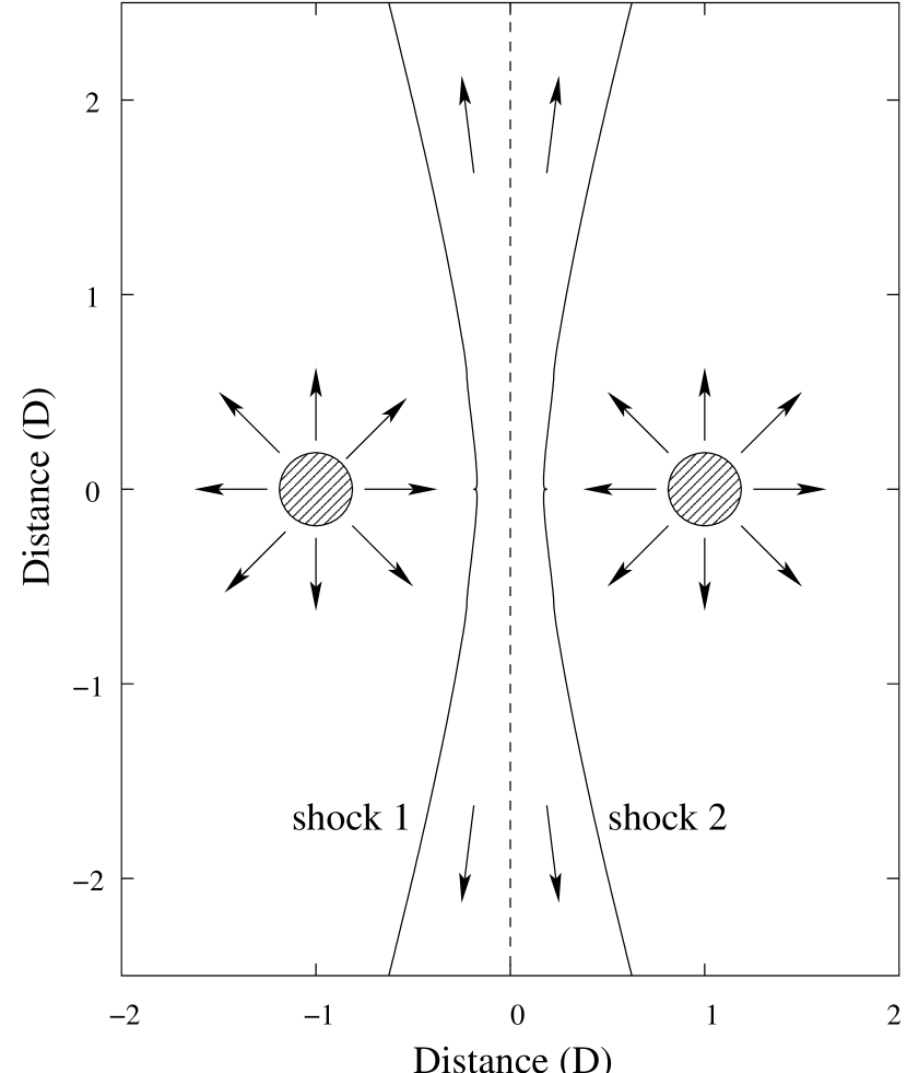
Figure 1: Sketch of a colliding-wind binary system in which the components (hatched) are the sources of identical hypersonic winds. The hot gas is bounded by two shocks (solid lines). The gas emanated from the different stars is separated by a contact surface (dashed line). The directions of gas flow are shown by arrows.

Figure 2: The shock wave (thick solid line) with the equation $y=y_{s}(x)$ in the coordinates $x$ and $y$ where the axis $x$ belong to the contact plane ($y=0$), and the axis $y$ coincides with the binary axis ($x=0$). A-point is the center of the star, and N is the point where the radial current line AN intersects the shock wave. The vector $\vec{k}$ is the tangent to the shock wave at the point N, and $t$ is the coordinate of the point N which is the length along the shock wave, measured from the binary axis to this point.

Figure 3: The shock shape in the zero (dashed curve), modified zero (dot-dashed curve), and first (dotted curve) approximations in the dimensionless coordinates $x$ and $y$ where the axis $x$ belong to the contact plane, and the axis $y$ coincides with the binary axis. The result of numerical simulations is represented by the solid curve.

References

• (1) Anders, E., & Grevesse, N. 1989, Geochim. Cosmochim. Acta, 53, 197
• (2) Antokhin, I.I., Owocki, S.P., & Brown, J. C. 2004, ApJ, 611, 434
• (3) Bairamov, Z.T., Pilyugin, N.N., & Usov, V.V. 1990, Soviet Astron., 34, 502
• (4) Barlow, M.J. 1982, in IAU Symp. 99, Wolf-Rayet Stars: Observations, Physics, Evolution, ed. C.W.H. de Loore and A.J. Willis (Dordrecht: Reidel), 149
• (5) Canto, J., Raga, A.C., Wilkin, F. P. 1996, ApJ, 469, 729
• (6) Chapman, J.M., Leitherer, C., Koribalski, B., Bouter, R., & Storey, M. 1999, ApJ, 518, 890
• (7) Cherepashchuk, A.M. 1976, Soviet Astr. Lett., 2, 138
• (8) Cherepashchuk, A. M. 2000, Ap&SS, 274, 159
• (9) Chernyi, G.G. 1961, Introduction to Hypersonic Flow (New York, London: Academic)
• (10) Chlebowski, T. 1989, ApJ, 342, 1091
• (11) Chlebowski, T., & Garmany, C.D. 1991, ApJ, 368, 241
• (12) Churchwell, E., Bieging, J.H., van der Hucht, K.A., Williams. P.M., Spoelstra, T.A.T., & Abbott, D.C. 1992, ApJ, 393, 329
• (13) Corcoran, M.F. 2003, in IAU Symp. 212, A Massive Star Odyssey: From Main Sequence to Supernova, ed. K.A. van der Hucht, A. Herrero, & E. Cesar (San Francisco: ASP), 130
• (14) Corcoran, M.F., Pittard, J.M., Stevens, I.R., Henley, D. B., & Pollock, A.M.T. 2005, in X-Ray and Radio Connections, ed. L.O. Sjouwerman & K.K. Dyer (Published electronically by NRAO, http://www.aoc.nrao.edu/events/xraydio), astro-ph/0406294
• (15) Corcoran, M.F., Stevens, I.R., Pollock, A.M.T., Swank, J.H., Shore, S.N., & Rawley, G.L. 1996, ApJ, 464, 434
• (16) Dessart, L., Crowther, P.A., Hillier, D.J., Willis, A.J., Morris, P.W., & van der Hucht, K. 2000, MNRAS, 315, 407
• (17) Dougherty, S.M., Williams, P.M., & Pollacco, D.L. 2000, MNRAS, 316, 143
• (18) Dougherty, S.M., Williams, P.M., van der Hucht, K.A., Bode, M.F., & Davis, R.J. 1996, MNRAS, 280, 963
• (19) Eichler, D., & Usov, V. 1993, ApJ, 402, 271
• (20) Freeman, N.C. 1956, J. Fluid Mech. 1, 366
• (21) Freeman, N.C. 1958, J. Fluid Mech. 4, 407
• (22) Galeev, A.A., Pilyugin, N.N., and Usov, V.V. 1989, in Proc. Varenna-Abastumani International School and Workshop on Plasma Astrophysics, Varenna, Italy (ESA SP-285), 125
• (23) Hayes, W.D. & Probstein, R.F. 1959, Hypersonic Flow Theory (New York: Academic Press)
• (24) Henley, D.B., Stevens, I.R., & Pittard, J.M. 2003, in IAU Symp. 212, A Massive Star Odyssey: From Main Sequence to Supernova, ed. K.A. van der Hucht, A. Herrero, & E. Cesar (San Francisco: ASP), 200
• (25) Henley, D.B., Stevens, I.R., & Pittard, J.M. 2005, MNRAS, 356, 1308
• (26) Jardine, M., Allen, H.R., & Pollock, A.M.T. 1996, A&A, 314, 594
• (27) Lebedev, M.G. & Savinov, K.G. 1969, Izvestiya Akademii Nauk SSSR, Mekhanika Zhidkosti i Gaza, No 3, 165
• (28) Luo, D., McCray, R., & Mac Low, M.-M. 1990, ApJ, 362, 267
• (29) Lunev, V.V. 1975, Hypersonic Aerodynamics (Moscow: Mashinostroenie)
• (30) Marchenko, S.V., Moffat, A.F.J., & Grosdidier, Y. 1999, ApJ, 522, 433
• (31) Moffat, A.F.J., Firmani, C., McLean, I.S., and Seggewiss, W. 1982, in IAU Symposium 99, Wolf-Rayet stars: observations, physics, evolution, eds. C.W.H. de Loore and A.J. Willis (Dordrecht: Reidel), 577
• (32) Monnier, J.D., Greenhill, L.J., Tuthill, P.G., & Danchi, W.C. 2002, ApJ, 566, 399
• (33) Monnier, J.D., Tuthill, P.G., & Danchi, W.C. 2002, ApJ, 567, 137
• (34) Moran, J.P., Davis, R.J., Spencer, R.E. Bode, M.F., & Taylor, A.R. 1989, Nature, 340, 449
• (35) Myasnikov, A.V., & Zhekov, S.A. 1991, Ap&SS, 184, 287
• (36) Niemela, V.S., Shara, M.M., Wallace, D.J., Zurek, D.R., & Moffat, A.F.J. 1998, AJ, 115, 2047
• (37) Pittard, J.M., & Stevens, I.R. 1997, MNRAS, 297, 383
• (38) Pittard, J.M., Dougherty, S.M., Coker, R.F., O’Connor, E., & Bolingbroke, N. J. 2006, A&A, 445, 1001
• (39) Pollock, A.M.T. 1987, ApJ, 320, 283
• (40) Pollock, A.M.T., Corcoran, M.F., Stevens, I.R., & Williams, P.M. 2005, ApJ, 629, 482
• (41) Prilutskii, O.F., & Usov, V.V. 1975, Astron. Cirk, No 854, 1
• (42) Prilutskii, O.F., & Usov, V.V. 1976, Soviet Astron., 20, 2
• (43) Savinov, K.G. 1975, PhD thesis, Moscow State University
• (44) Setia Gunawan, D.Y.A., de Bruyn, A.G., van der Hucht, K. A., & Williams, P.M. 2000, A&A, 356, 676
• (45) Stevens, I.R., Blondin, J.M., & Pollock, A.M.T. 1992, ApJ, 386, 265
• (46) Usov, V.V. 1990, Ap&SS, 167, 297
• (47) Usov, V.V. 1991, MNRAS, 252, 49
• (48) Usov, V.V. 1992, ApJ, 389, 635
• (49) Usov, V.V. 1995, in IAU Symp. 163, Wolf-Rayet Stars: Binaries, Colliding Winds, Evolution, ed. K.A. van der Hucht & P.M. Williams (Dordrecht: Kluwer), 495
• (50) Walder, R., & Folini, D. 2000, Ap&SS, 274, 343
• (51) White, R.L., & Becker, R.H. 1995, ApJ, 451, 352
• (52) Williams, P.M. 1999, in IAU Symp. 193, Wolf-Rayet Phenomena in Massive Stars and Starburst Galaxies, ed. K.A. van der Hucht, G. Koenigsberger, & P.R.J. Eenens (San Francisco: ASP), 267
• (53) Williams, P.M., & van der Hucht, K.A. 1992, in ASP Conf. Ser. 22, Nonisotropic and Variable Outflows from Stars, ed. L. Drissen, C. Leitherer, & A Nota (San Francisco: ASP), 269
• (54) Williams, P.M., van der Hucht, K.A., Morris, P.W., & Marang, F. 2003, in IAU Symp. 212, A Massive Star Odyssey: From Main Sequence to Supernova, ed. K.A. van der Hucht, A. Herrero, & E. C sar (San Francisco: ASP), 115
• (55) Williams, P.M., van der Hucht, K.A., Pollock, A.M.T., Florkowski, D.R., van der Woerd, H., & Wamsteker, W.M. 1990, MNRAS, 243, 662
• (56) Williams, P.M., van der Hucht, K.A., & Spoelstra, T.A.Th. 1994, A&A, 291, 805
• (57) Zel’dovich, Ya. B., & Raizer, Yu. P. 2002, Physics of Shock Waves and High-Temperature Hydrodynamic Phenomena (Mineola: Dover)
• (58) Zhekov, S.A., & Skinner, S.L. 2000, ApJ, 538, 808
Refer to caption