Gamma Ray Bursts as standard candles to constrain the cosmological parameters

Abstract

Gamma Ray Bursts (GRBs) are among the most powerful sources in the Universe: they emit up to $10^{54}$ erg in the hard X–ray band in few tens of seconds. The cosmological origin of GRBs has been confirmed by several spectroscopic measurements of their redshifts, distributed in the range $z\in(0.1,6.3)$. These two properties make GRBs very appealing to investigate the far Universe. Indeed, they can be used to constrain the geometry of the present day universe and the nature and evolution of Dark Energy by testing the cosmological models in a redshift range hardly achievable by other cosmological probes. Moreover, the use of GRBs as cosmological tools could unveil the ionization history of the universe, the IGM properties and the formation of massive stars in the early universe. The energetics implied by the observed fluences and redshifts span at least four orders of magnitudes. Therefore, at first sight, GRBs are all but standard candles. But there are correlations among some observed quantities which allows us to know the total energy or the peak luminosity emitted by a specific burst with a great accuracy. Through these correlations, GRBs becomes “known” candles, and then they become tools to constrain the cosmological parameters. One of these correlation is between the rest frame peak spectral energy $E_{\rm peak}$ and the total energy emitted in $\gamma$–rays $E_{\gamma}$, properly corrected for the collimation factor. Another correlation, discovered very recently, relates the total GRB luminosity $L_{\rm iso}$, its peak spectral energy $E_{\rm peak}$ and a characteristic timescale $T_{0.45}$, related to the variability of the prompt emission. It is based only on prompt emission properties, it is completely phenomenological, model independent and assumption–free. These correlations have been already used to find constraints on $\Omega_{\rm M}$ and $\Omega_{\Lambda}$, which are found to be consistent with the concordance model. The present limited sample of bursts and the lack of low redshift events, necessary to calibrate the correlations used to standardize GRBs energetics, makes the cosmological constraints obtained with GRBs still large compared to those obtained with other cosmological probes (e.g. SNIa or CMB). However, the newly born field of GRB–cosmology is very promising for the future.

1 Introduction

The present–day Universe and its past evolution are described in terms of a series of free parameters which combined together make up the cosmological model. One of the key objectives of observational cosmology is to exploit the power of combining different observations in order to test different cosmological models and find out the “best” one. The standard model of cosmology can have up to about 20 parameters needed to describe the background space–time, the matter content and the spectrum of the metric perturbations (e.g. [1, 2] ). However, a “minimal” subset of 7 parameters can be used to construct a successful cosmological model. In addition to the set of parameters describing the global geometry and dynamics of the Universe (in terms of its curvature and expansion rate - i.e. $\Omega_{M}$, $\Omega_{b}$, $\Omega_{k}$ and $h$), it became of greatest interest also the description of how the structure were formed from the basic constituents (described in terms of the perturbations amplitude $A$), the ionization history of the universe since the era of decoupling ($\tau$) and the description of how the galaxies trace the dark matter distribution on the largest scales (described in terms of the bias parameter $b$).

The goal of observational cosmology is to use astronomical objects and observations to derive the cosmological parameters (i.e. cosmological test - e.g [3, 4] ) once a cosmological model has been defined by selecting a set of parameters (i.e. the model selection problem - e.g. [1, 5]).

The Hubble constant $h=0.72\pm 0.1$ has been recently measured by the HST key project through the calibration of primary (Cepheid variables) and secondary (SN type I, SN type II, Galaxies) distance indicators within 600 Mpc. This measure has been confirmed by the CMB WMAP data and by large scale structure measures ([6],[7]).

Supernovae Ia, through the luminosity distance test (see below), have been used to constrain (combined with the evidence of a flat universe from CMB data) $\Omega_{M}\simeq 0.3$ and $\Omega_{\Lambda}\simeq 0.7$ (e.g. [9, 10, 11, 12]). One of the greatest breakthrough of the cosmological use of SNIa is the evidence of the recent re-acceleration of the universe (e.g. [13, 14, 15] see also [16] for a review), interpreted as the effect of a still obscure form of energy with negative pressure.

The CMB primary anisotropies bear the imprint of the physical conditions at the epoch of matter–radiation decoupling and of several effects such as the time-varying gravitational potential of structures along its propagation path (the ISW effect), the gravitational lensing and the scattering by the homogeneous ionized gas and by the collapsed–ionized gas (the SZ effect). Among the greatest breakthroughs of the CMB data analysis ([7]) it is worth mentioning that (i) the universe is flat, at the 1% level of accuracy, (ii) $\tau\sim 0.09\pm 0.03$, (iii) the power spectrum of the initial perturbations has the form of a scale invariant powerlaw, (iv) a static dark energy model is preferred. In particular the combination of the three year WMAP data with the Supernova Legacy data ([12]) yields a significant constrain on the dark energy equation of state, i.e. $w=-0.97\pm 0.02$, favouring the $\Lambda CDM$ cosmological model.

The study of the power spectrum of large galaxy surveys allowed to derive the baryon fraction $\Omega_{\rm b}/\Omega_{M}=0.185\pm 0.046$ ([17]) or, independently from the CMB priors, $\Omega_{M}=0.273\pm 0.025$ ([18]). Galaxy clustering analysis has also been used to put constraints, within the CDM model, on the neutrino mass (e.g. [19]). On the other hand Galaxy clusters, combined with constraints on the baryon density from primordial nucleosynthesis, have been used to constrain $\Omega_{M}$ and $h$ ([20]). Finally, strong (by clusters potentials) and weak gravitational lensing have been used to measure the mass power spectrum and derive constraints on $\sigma_{8}$ and $\Omega_{M}$ (e.g. [21]).

Gamma Ray Bursts are very promising for cosmology for, at least, two reasons: (i) they cover a very wide redshift range (see Fig. 1, solid black line) presently extending up to $z=6.29$ ([22], see [8]) and (ii) GRBs are detected by space instruments in the $\gamma$–ray band at energies $\geq$10 keV, i.e. their detection is free from the typical limitations due to dust extinction in the optical band.

The prospects of using GRBs as a new cosmological tool are exciting:

• similarly to QSO, GRBs might contribute to study the distribution and the properties of matter observed in absorption along the line of sight to these distant powerful sources (e.g. [23],[24],[25],[26]). Moreover, given the high luminosity of the early afterglow and the GRB transient nature, the absence of “proximity effects” (typical of QSO) makes GRBs powerful sources to study the metal enrichment and ISM properties of their own hosts ([27],[28], [29] see also [30]);

• if GRBs correspond to the death of very massive stars, they represent a unique probe of the initial mass function and of the star formation of massive stars ([31]) at very high redshifts;

• GRBs can be potentially detected at any redshift: the spectroscopic study of GRBs will help to define the properties of the IGM beyond the present QSO limits ($z\sim 6$) and, consequently to study the epoch(s) of re–ionization (e.g. [32], [33])

• the correlations between GRB spectral properties and collimation corrected energetics ([34],[35]), among prompt observables ([36]) and prompt and afterglow observables ([39]) have been shown to be powerful tools that “standardize” GRB energetics which can therefore be used to constrain the universe dark matter and and energy content ($\Omega_{\rm M}$,$\Omega_{\Lambda}$) and the nature of dark energy ([34],[41],[42],[39],[43], [44]).

GRBs are not alternative to SN Ia or other cosmological probes. On the contrary, they are complementary to them, because of their different redshift distribution and because any evolutionary properties would likely to act differently on GRBs than on SN Ia or other probes and because the joint use of different cosmological probes is the key to break the degeneracies in the found values of the cosmological parameters.

1.1 The standard candle test

The classical methods used to test the cosmological models are: (i) the luminosity distance test (mainly applied to SN Ia), (ii) the angular–size distance test (whose modern application consists in the study of the CMB anisotropies) and (iii) the volume test based on galaxy number count. Besides there are cosmological tests aimed at testing structures’ formation models such as the study of the power spectrum of luminous matter or of the amplitude of the present–day mass fluctuations.

For an object with known and fixed luminosity $L$, not evolving with cosmic time, and measured flux $F$, we can define its luminosity distance $D_{L}=(L/4\pi F)^{1/2}$ which is related to the radial coordinate $r$ of the Friedman–Robertson–Walker metric by $D_{L}=r/a(\tau)=r\,(1+z)$ (where $a(\tau)$ is the scale factor as a function of the comoving time, $\tau=t\,H_{0}$). Therefore, $D_{L}$ depends upon the expansion history and curvature of the universe through the radial coordinate $r$. By measuring the flux of “standard candles” as a function of redshift, $F(z)$, we can perform the classical luminosity distance test by comparing $D_{L}$, obtained from the flux measure, with $D_{L}(\bar{p})$ predicted by the cosmological model, where $\bar{p}$ is a set of cosmological parameters (e.g. $\Omega_{M}$, $\Omega_{\Lambda}$ and $h$).

This test has been widely used with SNIa (see [45] for a recent review). The high peak luminosity (i.e. $\sim 10^{10}L_{\odot}$) of SNIa makes them detectable up $z>$1. However, SNIa, strictly–speaking, are not standard candles: their absolute peak magnitude varies by $\sim 0.5$ mag which corresponds to a variation of 50%–60% in luminosity. In the early 1990s ([46],[47],[48],[49]) it was discovered a tight correlation between the peak luminosity of SNIa and the rate at which their luminosity decays in the post–peak phase. This is known as the “stretching–luminosity correlation” and in its simplest version is $M_{B}\simeq 0.8(\Delta m_{15}-1.1)-19.5$, where $M_{B}$ is the B–band absolute magnitude and $\Delta m_{15}$ represents the decrease of the magnitude from the time of the peak and 15 days later. The application of this correlation reduces the luminosity spread of SNIa to within 20% and makes them usable as cosmological tools ([48]).

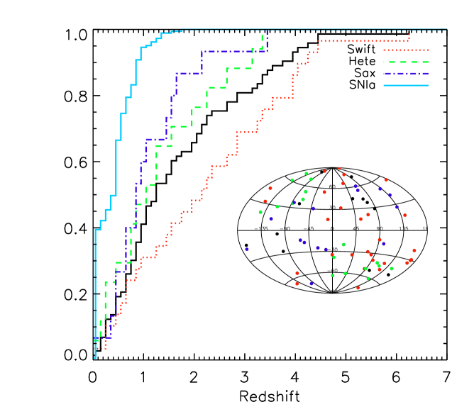
Figure 1: Normalized redshift distribution of 79 long duration GRBs updated to Jan 2006 (solid–black histogram). Also shown are the distributions separated according to three different satellites that detected most of these burst ($BeppoSAX$ [15 GRBs, dot-dashed blue line], Hete-II [17 GRBs, dashed–green line] and Swift [29 GRBs, dotted–red line]). The redshift distribution of the “Gold” SNIa sample (156 objects) of [11] is also shown (solid–blue line). The insert shows the sky distribution, in galactic coordinates, of the present sample of GRBs with spectroscopically measured redshifts (see http://www.mpe.mpg.de/  jcg/grbgen.html for reference).

The situation with GRBs is remarkably similar. At first glance the wide dispersion of their energetics prevented their use as cosmological probes even when accounting for their “jetted” geometry (Sec. 2). Several intrinsic correlations between temporal or spectral properties and GRB isotropic energetics and luminosities (Sec. 3) have been regarded as a possibility to make GRBs cosmological tools. However, only by accounting for a third variable (which in the standard model measures the GRB jet opening angle - Sec. 4), GRBs became a new class of “standard candles” (or, better, “known” candles). The constraints on the cosmological parameters obtained by the luminosity distance test applied to GRBs are less severe than what obtained with SNIa (Sec. 5). This is mainly due to the presently still limited (i.e. only 19) number of GRBs with well determined prompt and afterglow properties that can be used as standard candles (Sec. 9).

2 GRB energetics and luminosities

The cumulative redshift distribution of long GRBs is compared in Fig. 1 with that of 156 SNIa ([11]). We also show the different redshift distributions obtained with the GRBs detected by the three different satellites Swift, BeppoSAX and Hete–II. The better sensitivity and faster accurate afterglow localization of Swift ([51]), compared to BeppoSAX and Hete–II, might account for the detection, on average, of fainter X–ray and Optical afterglows and, therefore, for systematically larger redshifts ([52]). It should also be noted that due to its soft energy band (15–150 keV), Swift might better detect and localize soft/dim long bursts. The insert of Fig. 1 shows that the sky distribution of the population of bursts with measured $z$ is consistent with that of long GRBs detected by BATSE (see e.g. [54]).

2.1 Isotropic energy and luminosity

The energy ($E$) and luminosity ($L$) of GRBs with measured redshifts can be estimated through the burst observed fluence ($S$, i.e. the flux integrated over the burst duration) and peak flux ($P$). If GRBs emit isotropically, the energy radiated during their prompt phase is $E_{\rm iso}=4\pi D_{L}^{2}S/(1+z)$ [where the term (1+z) accounts for the cosmological time dilation effect] and the isotropic luminosity is $L_{\rm iso}=4\pi D_{L}^{2}P$. Fig. 2 (upper panel) shows the distribution of $E_{\rm iso}$ (orange–filled histogram) obtained with the most updated sample of 44 GRBs ([55]) with measured redshifts and measured spectral properties (from which the bolometric fluence in the 1–10⁴ keV rest frame energy band can be computed). In the same plot we also show the distribution of $L_{\rm iso}$ (blue–hatched histogram) which has been obtained by updating the compilation of [56] with the most recent events. Note that the bolometric luminosity is often computed by combining the peak flux (relative to the peak of the GRB lightcurve) with the spectral data derived from the analysis of the time integrated spectrum. As discussed in [56] this is strictly correct only if the GRB spectrum does not evolve in time during the burst, contrary to what is typically observed ([57]).

If the GRB energy and luminosity distributions of Fig. 2 (upper panel) are modeled with gaussian functions (solid–red line and solid–green line, respectively), we find that the average isotropic energy of GRBs is $\langle Log(E_{\rm iso})\rangle=53.03\pm 0.89$ while the average luminosity is $\langle Log(L_{\rm iso})\rangle=52.23\pm 0.10$ (1$\sigma$ uncertainty). Clearly, this large dispersion of $E_{\rm iso}$ and $L_{\rm iso}$ prevents the application of the luminosity distance test to GRBs.

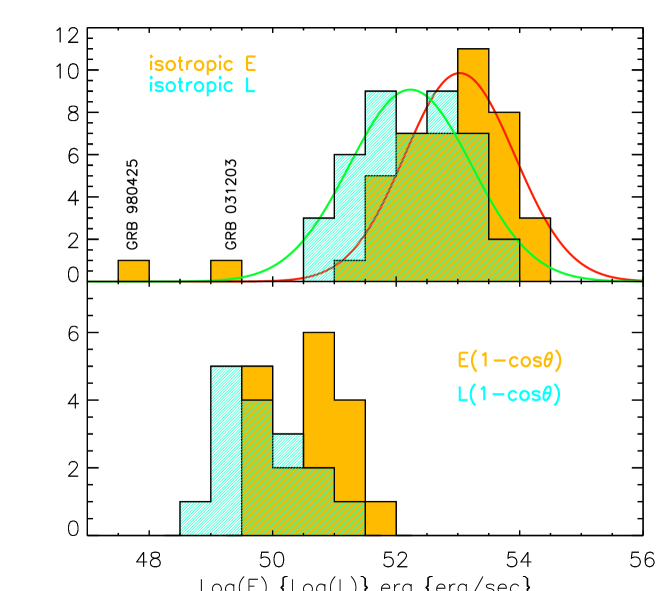
Figure 2: Upper panel: distributions of the isotropic equivalent energy $E_{\rm iso}$ (orange–filled histogram) and of the isotropic equivalent luminosity $L_{\rm iso}$ (blue-hatched histogram). The sample comprises the 44 long GRBs with measured redshifts and well determined spectral properties. The values of $E_{\rm iso}$ are taken from [55] while $L_{iso}$ is from [56] (updated with the most recent bursts). The solid lines represent the Gaussian fit to these distributions. The two low–luminosity bursts (980425 and 031203) are also shown (see [34], [55]). Lower panel: distributions of the collimation corrected energy (orange–filled histogram) and luminosity (blue–hatched histogram). The samples comprises only the 19 GRBs with firm measurements of the jet break time from which the jet opening angle could be computed (18 bursts from [35] updated with GRB 051022, see [44]).

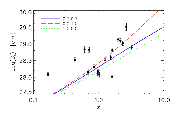
Figure 3: Hubble diagram for GRBs with measured redshifts and jet break time assuming a unique value of the collimation corrected energy $E_{\gamma}=8.8\times 10^{50}$ erg, i.e. the central value of its distribution (blue–hatched histogram of Fig.3, lower panel). The luminosity distance is obtained by solving the equation $E_{\gamma}$=const=$E_{\rm iso}(1-\cos\theta)$.

2.2 Collimation corrected energy and luminosity

A considerable reduction of the dispersion of GRBs energetics has been found by [58] (later confirmed by [59]) when they are corrected for the collimated geometry of these sources.

Theoretical considerations on the extreme GRB energetics under the hypothesis of isotropic emission ([60],[61]) led to think that, similarly to other sources, also GRBs might be characterized by a jet. In the standard scenario, the presence of a jet ([62], [63], [64] affects the afterglow lightcurve which should present an achromatic break few days after the burst (see Sec. 4 for more details).

Indeed, the observation of the afterglow lightcurves allows us to estimate the jet opening angle $\theta_{\rm jet}$ from which the collimation factor can be computed, i.e. $f=(1-\cos\theta_{\rm jet})$. This geometric correction factor, applied to the isotropic energies ([58]) led to a considerable reduction of the GRB energetics and of their dispersion. Fig. 2 (lower panel) shows the distributions of the collimation corrected energy and peak luminosity ($E_{\gamma}=E_{\rm iso}\cdot f$ and $L_{\gamma}=L_{\rm iso}\cdot f$, respectively) for the updated sample of bursts with measured $\theta_{\rm jet}$. When compared with the parent distributions of the isotropic quantities (upper panel of Fig. 2) we note that, also accounting for the collimation factor, both $E_{\gamma}$ and $L_{\gamma}$ are spread over $\sim$3 orders of magnitudes.

However, given the slightly lower dispersion of the collimation corrected energies and luminosities (bottom panel of Fig. 2) with respect to their isotropic equivalent (upper panel of Fig. 2), it is worth to verify if GRBs can be effectively used as standard candles. The simplest test consists in building the Hubble diagram (see also [59],[40]). By assuming the central value of the collimation corrected energy, i.e. $E_{\gamma}=8.8\times 10^{50}$ erg, for all the GRBs with measured $z$ and $\theta_{\rm jet}$, it is possible to derive their luminosity distance as if they were strictly speaking standard candles, i.e. characterized by a unique luminosity. By solving numerically the equation $E_{\gamma}=8.8\times 10^{50}=E_{\rm iso}\cdot[1-\cos\theta_{\rm jet}]$ (where also $\theta_{\rm jet}$ depends on $D_{\rm L}$ through $E_{\rm iso}$, see Sec. 4) we derive the luminosity distance which is plotted versus redshift in Fig. 3. Note that the scatter of the data points is larger than the separation of different cosmological models (lines in Fig. 3). This simple tests shows that, even if the collimation correction reduces the dispersion of GRB energies, they cannot still be used as “standard candles” for the luminosity distance test.

3 The intrinsic correlations of GRBs

For GRBs with known redshifts we can study their rest frame properties. Although still based on a limited number (few tens) of events, this analysis led to the discovery of several correlations involving GRBs rest frame properties. In the following sections these correlations are summarized.

3.1 The Lag–Luminosity correlation ($\tau$-$L_{\rm iso}$)

The analysis of the light curves of GRBs observed by BATSE in 4 broad energy ranges (i.e.roughly 25-50, 50-100, 100-300 and $\geq$300 keV), led to the discovery of spectral lags: the emission in the higher energy bands precedes that in the lower energy bands ([65]). The time lags typically range between 0.01 and 0.5 sec (even few seconds lags have been observed - [66]) and there is no evidence of any trend, within multipeaked GRBs, between the lags of the initial and the latest peaks ([67]). It has been proposed that the lags are a consequence of the spectral evolution (e.g.[68]), typically observed in GRBs ([69]), and they have been interpreted as due to radiative cooling effects ([70]). Alternative interpretations invoke geometric (i.e. viewing angle) and hydrodynamic effects ([71], [72]) within the standard GRB model.

In particular, the analysis of the temporal properties of GRBs with known redshifts revealed a tight correlation between their spectral lags ($\tau$) and the luminosity ($L_{\rm iso}$) ([73]): more luminous events are also characterized by shorter spectral lags as represented in Fig.4 (left panel) where the original correlation $\tau\propto L_{iso}^{-0.8}$, found with 6 GRBs, is reported (see also Tab.1).

Possible interpretations of the Lag-Luminosity correlation include the effect of spectral softening of GRB spectra ([74], [75]) during the prompt due to radiative cooling ([76], [77]) or a kinematic origin due to the variation of the line–of–sight velocity in different GRBs ([78]) or to the viewing angle of the jet ([79]).

Moreover, the $\tau-L_{iso}$ correlation has been used as a pseudo-redshift indicator to estimate $z$ for a large population of GRBs ([80]) and also to study the GRB population properties (i.e. jet opening angle, luminosity function and redshift distribution) within a unifying picture ([66]).

3.2 The Variability–Luminosity correlation ($V$-$L_{\rm iso}$)

The light curves of GRBs show several characteristic timescales. Since their discovery, it was recognized that the $\gamma$–ray emission can vary by several orders of magnitudes (i.e. from the peak to the background level) on millisecond (or even lower ([82]) timescales (e.g [81]). Also the afterglow emission presents some variability on timescales of a few seconds (e.g.[83],[84]). The analysis of large samples of bursts also showed the existence of a correlation between the GRB observer frame intensity and its variability ([81]). A short timescale variability during the prompt emission of GRBs has been considered as a strong argument against the external shock model, favouring, instead, an internal shock origin for the burst high energy emission (e.g. [85]). In fact, the rapid variation of the emission was interpreted as a signature of a discontinuous and rapidly varying activity of the inner engine that drives the burst ([86]). This is hardly produced by a decelerating fireball in the external medium. However, alternative scenarios propose an external origin of the observed variability as due to the shock formation by the interaction of the relativistically expanding fireball and variable size ISM clouds ([87]).

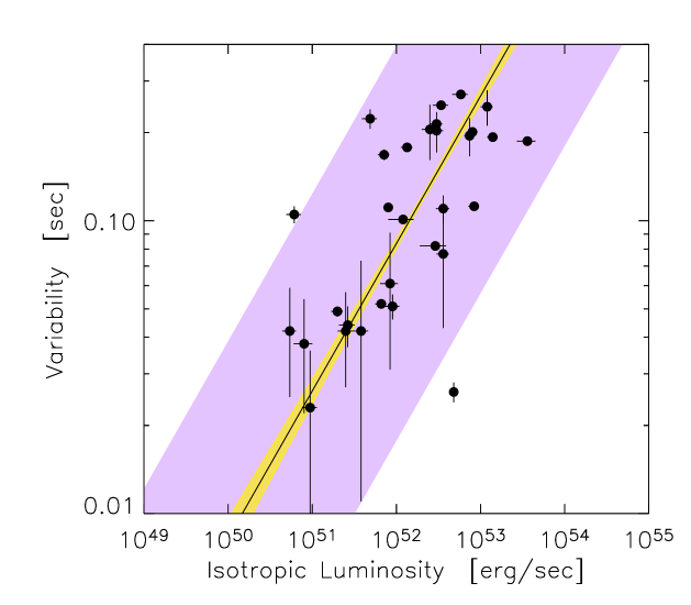
Figure 4: Left: Lag–Luminosity correlation (data from [65]) for 6 GRBs with measured redshift. The best fit (solid line) is also shown. Right: Variability–luminosity correlation for the sample of 31 GRB of [90]. The violet–shaded region represents the 3$\sigma$ scatter of the data points around the best correlation (solid line).

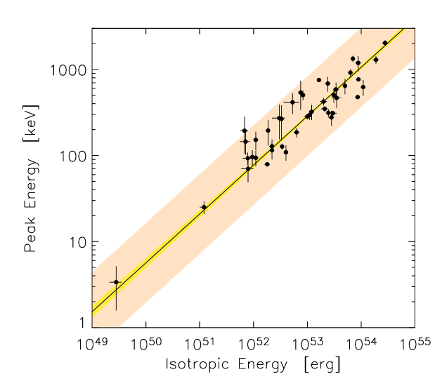
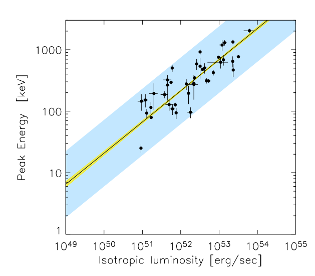
Figure 5: Left: Peak energy–isotropic energy correlation. Data are from [55]. The orange shaded region represents the 3$\sigma$ scatter of the data points around the correlation (solid line). Right: Peak energy–isotropic luminosity correlation. Data (40 GRBs) are from [105] updated with the most recent bursts. The blue shaded region represents the 3$\sigma$ scatter of the data points around the correlation (solid line).

Table 1: GRB intrinsic correlations involving isotropic quantities. N: number of GRBs used to find the correlation. The rank correlation coefficient $r_{s}$ and its chance probability $P$ are given. The best fit parameters of the powerlaw model (normalization $q$ and slope $\alpha$), with their 1$\sigma$ uncertainty, are also reported together with the $\chi^{2}$(dof).

Isotropic Correlations	N	$r_{s}$	$P$	$q$	$\alpha$	$\chi^{2}$(dof)
Lag-Luminosity	6	-0.82	0.06	39.09$\pm$7.2	-0.77$\pm$0.13	…
$Log(\tau_{\rm lag})=q+\alpha Log(L_{\rm iso})$
Variability-luminosity	31	0.61	8$\times 10^{-4}$	-27.3$\pm$1.3	0.5$\pm$0.02	1252(29)
$Log(V)=q+\alpha Log(L_{\rm iso})$
Peak energy-Isotropic energy	43	0.89	$10^{-15}$	-27.64$\pm$0.65	0.56$\pm$0.01	493(41)
$Log(E_{\rm peak})=q+\alpha Log(E_{\rm iso})$
Peak energy-Isotropic luminosity	40	0.86	$10^{-11}$	-27.02$\pm$0.56	0.50$\pm$0.01	454(38)
$Log(E_{\rm peak})=q+\alpha Log(L_{\rm iso})$

Fenimore & Ramirez–Ruiz ([88]) and Reichart et al. ([89]) found a correlation between GRB luminosities ($L_{\rm iso}$) and their variability ($V$): more luminous bursts have a more variable light curve. The $V-L_{\rm iso}$ correlation has been recently updated ([90]) with a sample of 31 GRBs with measured redshifts. This correlation has also been tested ([91]) with a large sample of 551 GRBs with only a pseudo-redshift estimate (from the lag–luminosity correlation - [80]). An even tighter correlation (i.e. with a reduction of a factor 3 of its scatter) has been derived ([92]) by slightly modifying the definition of the variability first proposed by [89]. In Fig.4 we show the data points (from [90]) which show the existence of a statistically significant correlation (with rank correlation coefficient $r_{s}=-0.6$ and chance correlation probability $P=8\times 10^{-4}$). We fitted this correlation by accounting for the errors on both coordinates and the best fit coefficients are reported in Tab.1. The scatter of the data points around this correlation (computed perpendicular to the correlation itself) can be modeled with a gaussian with $\sigma=0.24$. As also shown in Fig.4 (right panel) such a large scatter is responsible for a statistically poor fit, as shown by the resulting $\chi^{2}$=1252/29. However, as discussed in [93] when the sample variance (see also [89], [94] ) is taken into account ($\sigma_{logV}=0.20\pm 0.04$) the correlation is $L\propto V^{3.4(+0.9,-0.6)}$ with a reduced $\chi^{2}_{r}\sim 1$.

3.3 The spectral peak energy–isotropic energy correlation ($E_{\rm peak}$-$E_{\rm iso}$)

It has been shown ([95]) that GRBs with highly variable light curves have larger $\nu F_{\nu}$ spectral peak energies. The existence of a $V$-$E_{\rm peak}$ correlation and of the variability–luminosity correlation ($V$-$L_{\rm iso}$) implies that the rest frame GRB peak energy $E_{\rm peak}$ is correlated with the intrinsic luminosity of the burst. Amati et al. ([96]) analyzed the spectra of 12 $BeppoSAX$ GRBs with spectroscopically measured redshifts and found that the isotropic–equivalent energy $E_{iso}$, emitted during the prompt phase, is correlated with the rest–frame peak energy of the $\gamma$–ray spectrum $E_{\rm peak}=E_{\rm peak}^{\rm obs}(1+z)$. Such a correlation was later confirmed with GRBs detected by BATSE, Hete-II and the IPN satellites and extended with X-ray Flashes (XRF) towards the low end of the $E_{\rm peak}$ distribution ([97],[34],[53]). Recently the $E_{\rm peak}$-$E_{\rm iso}$ correlation has been updated with a sample of 43 GRBs (comprising also 2 XRF) with firm estimates of $z$ and of the spectral properties ([55]). In Fig. 5 we show the $E_{\rm peak}$–$E_{\rm iso}$ correlation with the most updated sample of GRBs reported in [55]. The best fit correlation parameters are reported in Tab.1. The scatter of the data points around the $E_{\rm peak}$-$E_{\rm iso}$ correlation can be modeled with a Gaussian of $\sigma\sim 0.15$.

The theoretical interpretations, proposed so far, of the $E_{\rm peak}$–$E_{\rm iso}$ correlation ascribe it to geometrical effects due to the jet viewing angle with respect to a ring–shaped emission region ([98],[99]) or with respect to a multiple sub-jet model structure which also accounts for the extension of the above correlation to the X-ray Rich (XRR) and XRF classes ([100],[101]). An alternative explanation of the $E_{\rm peak}$–$E_{\rm iso}$ correlation is related to the dissipative mechanism responsible for the prompt emission ([102]): if the peak spectral energy is interpreted as the fireball photospheric thermal emission comptonized by a dissipation mechanism (e.g. magnetic reconnection or internal shock) taking place below the transparency radius, the observed correlation can be reproduced.

3.4 The peak spectral energy–isotropic luminosity correlation ($E_{\rm peak}$-$L_{\rm iso}$)

A correlation between $E_{\rm peak}$ and the isotropic luminosity $L_{\rm iso}$ (i.e. $E_{\rm peak}\propto L_{\rm iso}^{0.5}$) has been discovered ([109]) with a sample of 16 GRBs. A larger sample of 25 GRBs confirmed this correlation ([56]), although with a slightly larger scatter of the data points. We have further updated this sample to 40 GRBs with known redshifts and Fig. 5 (right panel) shows the $E_{\rm peak}$–$L_{\rm iso}$ correlation found with this sample. In Tab.1 are reported the fit results of the $E_{\rm peak}-L_{\rm iso}$ correlation. The scatter of the data points around this correlation (see Fig.12) can be modeled with a Gaussian of $\sigma\simeq 0.2$. Also in this case, as discussed for the $E_{\rm peak}-E_{\rm iso}$ ([55]) the resulting reduced $\chi^{2}$ is quite large unless accounting for a sample variance of the order of $\sim 0.13$.

As discussed in [108], the luminosity $L_{\rm iso}$ is defined by combining the time–integrated spectrum of the burst with its peak flux (also $E_{\rm peak}$ is derived using the time integrated spectrum). This assumes that the time–integrated spectrum is also representative of the peak spectrum. However, it has been shown that GRBs are characterized by a considerable spectral evolution (e.g. [68]). If the peak luminosity is derived only by considering the spectrum integrated over a small time interval ($\sim 1$ sec) centered around the peak of the burst light curve , we find a larger dispersion of the $E_{\rm peak}$-$E_{\rm iso}$ correlation (see [108]). This suggests that, in general, the time averaged quantities (i.e. the peak energy of the time integrated spectrum and the “peak–averaged” luminosity) are better correlated than the “time–resolved” quantities.

Schaefer ([110]) combined the Lag–Luminosity and the Variability–Luminosity relations of 9 GRBs to build their Hubble diagram. He showed that GRBs might be powerful cosmological tools. However, some notes of caution should be addressed when using the correlations presented in Tab.1 for cosmographic purposes. In fact, one fundamental condition is that there exist at least one cosmology in which these correlations give a good fit, i.e. a reduced $\chi^{2}_{red}\simeq 1$ and, unless accounting for the sample variance, this is not the case for the correlations presented so far.

3.5 The isotropic luminosity–peak energy–high signal timescale correlation ($L_{\rm iso}$–$E_{\rm peak}$–$T_{0.45}$)

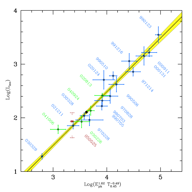
Figure 6: Multi variable linear regression analysis of the $L_{\rm iso}$-$E_{\rm peak}$-$T_{0.45}$ correlation based on 19 GRBs. The open circles represent the 19 bursts used for the fit (solid line). The solid filled region represents the 1$\sigma$ uncertainty on the best fit (see Eq. 1). The fit is performed in the centroid defined by the data points (solid circle) where the errors on the best fit parameters are uncorrelated. GRB 050525 was not used for the multi–variable regression analysis due to its uncertain luminosity.

A new correlation recently discovered by Firmani et al. ([36]) relates three observables of the GRB prompt emission. These are the isotropic luminosity $L_{\rm iso}$, the rest frame peak energy $E_{\rm peak}$ and the rest frame “high signal” timescale $T_{0.45}$. The latter is a parameter which has been previously used to characterize the GRB variability (e.g. [89]) and represents the time spanned the brightest 45% of the total counts above the background. Through the analysis of 19 GRBs, for which $L_{\rm iso}$ $E_{\rm peak}$ and $T_{0.45}$ could be derived, [36] found that $L_{\rm iso}\propto E_{\rm peak}^{1.62}\cdot T_{0.45}^{-0.49}$ with a very small scatter. This correlation is presented in Fig.6.

The $L_{\rm iso}-E_{\rm peak}-T_{0.45}$ correlation is based on prompt emission properties only and it has some interesting consequences: (i) it represents a new powerful (redshift) indicator for GRBs without measured redshifts, which could be computed only from the prompt emission data (spectrum and light curve); (ii) it represents a new powerful cosmological tool ([37] - see Sec. 6.2) which is model independent (differently from the $E_{\gamma}-E_{\rm peak}$ correlation (see Sec. 5) which relies on the standard GRB jet model); (iii) it is “Lorentz invariant” for normal fireballs, i.e. when the jet opening angle is $\theta_{\rm jet}>1/\Gamma$. In this case, in fact, the luminosity scales as $\delta^{-2}$ when it is transformed from the rest to the comoving frame and the doppler factor cancels out with that of the peak energy and of $T_{0.45}$ - see [36].

4 The third observable: the jet break time ($t_{\rm break}$)

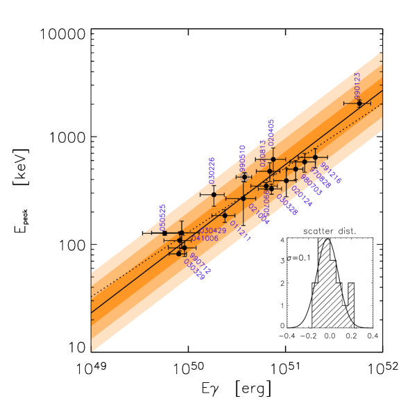
Figure 7: The $E_{\rm peak}$–$E_{\gamma}$ correlation from [35] obtained under the assumption that the circum burst medium has a constant density. The 18 bursts are those with measured redshift and firm measurements of their spectral properties. The best powerlaw fit of the data points, obtained by accounting for the uncertainties on both coordinates, is shown (solid line) together with the linear regression analysis, i.e. without accounting for the data uncertainties (dotted line). The scatter of the data points around the best fit correlation is shown in the insert with its Gaussian fit. The 1,2 and 3$\sigma$ scatter of the data points around the best correlation is represented by the shaded region.

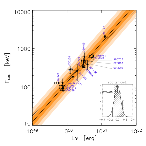
Figure 8: The $E_{\rm peak}$–$E_{\gamma}$ correlation in the case of a wind profile of the external medium density as found with the 18 GRBs reported in [35]. The solid line represents the best fit powerlaw model obtained accounting for the errors on both coordinates. We also show the fit obtained with the simplest linear regression, i.e. without accounting for the errors on the coordinates (dotted line), which has a slope of 0.92. The circled point represents GRB 030326 which is giving the largest contribution (23%) to the best fit reduced $\chi^{2}$. The shaded regions represent the 1, 2 and 3$\sigma$ scatter around the best fit correlation. The names of the 18 GRBs are indicated. The insert reports the distribution (hatched histogram) of the scatter of the data points computed perpendicular to the best correlation (solid line in the main plot) and its gaussian fit (solid line in the insert) which has a $\sigma=0.08$.

As shown above the correlations between the spectral peak energy and the isotropic energy or luminosity are too much scattered to be used as distance indicators. Only the $L_{\rm iso}$–$E_{\rm peak}$–$T_{0.45}$, which is based on prompt emission properties, is sufficiently tight to standardize GRB energetics (as it will be shown in Sec. 5 and Sec. 6).

However, all the above correlations have been derived under the hypothesis that GRBs are isotropic sources. Indeed, the possibility that GRB fireballs are collimated was first proposed for GRB 970508 ([60]) and subsequently invoked for GRB 990123 as a possible explanation for their extraordinarily large isotropic energy ([61]). The main prediction of the collimated GRB model is the appearance of an achromatic break in the afterglow light curve which, after this break time, declines more steeply than before it ([62], [63]). Due to the relativistic beaming of the photons emitted by the fireball, the observer perceives the photons within a cone with aperture $\theta_{\Gamma}\propto 1/\Gamma$, where $\Gamma$ is the bulk Lorentz factor of the material responsible for the emission. During the afterglow phase the fireball is decelerated by the circum burst medium and its bulk Lorentz factor decreases, i.e. the beaming angle $\theta_{\Gamma}$ increases with time. A critical time is reached when the beaming angle equals the jet opening angle, i.e. $\theta_{\Gamma}\sim 1/\Gamma\sim\theta_{\rm jet}$, i.e. when the entire jet surface is visible . Under such hypothesis the jet opening angle $\theta_{\rm jet}$ can be estimated through this characteristic time ([63]), i.e. the so called jet–break time $t_{\rm break}$ of the afterglow light curve. Typical $t_{\rm break}$ values ranges between 0.5 and 6 days ([58],[59],[34])

Table 2: GRB intrinsic correlations involving collimation corrected quantities. N: number of GRBs used to find the correlation. The rank correlation coefficient $r_{s}$ and its chance probability $P$ are given. The best fit parameters (with their 1$\sigma$ uncertainty) are also reported together with their $\chi^{2}$(dof).

Coll. corrected Correlations	N	$r_{s}$	$P$	$q$	$\alpha$	$\beta$	$\chi^{2}$(dof)
$Log(E_{\rm peak})=q+\alpha Log(E_{\gamma,HM})$	18	0.9	2.3$\times 10^{-8}$	-32.36$\pm$2.27	0.69$\pm$ 0.04		22.4(16)
$Log(E_{\rm peak})=q+\alpha Log(E_{\gamma,WM})$	18	0.92	6.8$\times 10^{-8}$	-49.44$\pm$3.27	1.03$\pm$0.06		18(16)
$Log(E_{\rm peak})=q+\alpha Log(E_{\rm iso})$	18			-48.05$\pm$0.24	1.93$\pm$0.11	-1.08$\pm$0.17	24.2(16)
…… $+\beta Log(t_{\rm break})$
$Log(E_{\rm peak})=q+\alpha Log(L_{\gamma,HM})$	16	0.9	4$\times 10^{-4}$	-22.8$\pm$1.3	0.51$\pm$0.03		41(14)
$Log(E_{\rm peak})=q+\alpha Log(L_{\gamma,WM})$	16	0.9	7$\times 10^{-4}$	-35.1$\pm$2.0	0.75$\pm$0.04		76(14)

The jet opening angle can be derived from $t_{\rm break}$ in two different scenarios (e.g. [111]): (a) assuming that the circum burst medium is homogeneous (HM) or (b) assuming a stratified density profile (WM) produced, for instance, by the wind of the GRB progenitor. In both cases the jet is assumed to be uniform.

5 The peak energy–collimation corrected energy correlation ($E_{\rm peak}$-$E_{\gamma}$)

By correcting the isotropic energy of GRBs with measured redshifts, under the hypothesis of a homogeneous circum–burst medium, Ghirlanda et al. ([34]) discovered that the collimation corrected energy $E_{\gamma}=E_{\rm iso}(1-\cos\theta_{\rm jet})$ is tightly correlated with the rest frame peak energy. With an initial sample of 15 GRBs ([34]) this correlation results steeper ( i.e. $E_{\rm peak}\propto E_{\gamma}^{0.7}$) than the corresponding correlation involving the isotropic energy and with a very small scatter (i.e. $\sigma\sim 0.1$ to be compared with the $\sim 0.2$ scatter of the correlation with $E_{\rm iso}$). The addition of new GRBs (some of which also discovered by Swift and, at least, by another IPN satellite in order to have an estimate of the peak energy) has confirmed this correlation and its small scatter (e.g. [105]).

Recently, Nava et al. ([35]) reconsidered and updated the original sample of GRBs with firm estimate of their redshift, spectral properties and jet break times. With the most updated sample of 18 GRBs we can re-compute the $E_{\rm peak}$–$E_{\gamma}$ correlation in the HM case. This is represented in Fig.7 and results $E_{\rm peak}\propto E_{\gamma}^{(0.69\pm 0.04)}$ (see Tab.2) with a very small scatter (i.e. $\sigma\sim 0.1$). Only two bursts (i.e. GRB 980425 and GRB 031203 - which are not reported in the figures - but see [105]) are outliers to this correlation, as well as to the $E_{\rm peak}$-$E_{\rm iso}$ correlation. Possible interpretations has been put forward such as the possibility that these events are seen out of their jet opening angle ([112]) and therefore appear de-beamed in both $E_{\rm peak}$ and $E_{\rm iso}$ (see also [113]). However, other possible explanations could be considered ([114],[115]).

Most intriguingly, [35] also computed the $E_{\rm peak}$–$E_{\gamma}$ correlation in the WM case where a typical $r^{-2}$ density profile is assumed. The resulting correlation is reported in Fig.8. The $E_{\rm peak}$-$E_{\rm gamma}$ correlation derived in the WM case has two major properties: (i) its scatter, i.e. $\sigma=0.08$, is smaller than in the HM case (although, due to the still limited number of data points, this does not represent a test for the WM case against the HM case) and (ii) it is linear, i.e. $E_{\rm peak}\propto E_{\gamma}$. Under the hypothesis that our line of sight is within the GRB jet aperture angle, the existence of a linear $E_{\rm peak}$-$E_{\gamma}$ correlation also implies that it is invariant when transforming from the source rest frame to the fireball comoving frame. A striking, still not explained, consequence of this property is that the total number of photons emitted in different GRBs is similar and should correspond to $\sim 10^{57}$ i.e. roughly the number of baryons in 1 solar mass. The latter property might have important implications for the understanding of the dynamics and radiative processes of GRBs.

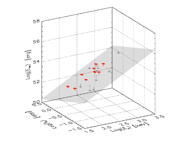
Figure 9: The 3-D representation of the $E_{\rm peak}$–$E_{\rm iso}$–$t_{\rm break}$ correlation computed with the updated sample of [35]. The shaded plane represents the best fit correlation and the data points are marked differently if the lie above (red points) or below (gray stars) this plane. The vertical lines show the distance of the data points from the best fit plane.

One of the major criticism encountered by the above correlations between the peak energy and the collimation corrected energy is the fact that the collimation correction is derived from the measure of $t_{\rm break}$ by assuming the standard fireball model. If on the one hand the small scatter of the $E_{\rm peak}$-$E_{\gamma}$ correlation might be, in turn, regarded as a confirm of this model, on the other hand it could still be a matter of debate when these correlations are used for cosmographic purposes.

6 The peak energy–isotropic energy–jet break time correlation ($E_{\rm peak}$-$E_{\rm iso}$-$t_{\rm break}$)

A completely empirical correlation also links the same three observables used in deriving the above $E_{\rm peak}$-$E_{\gamma}$ correlation. Liang & Zhang ([39]), in fact, found that the peak energy $E_{\rm peak}$, the jet break time $t_{\rm break}$ and the isotropic energy $E_{\rm iso}$ are correlated. In Fig.9, we report the 3-D correlation obtained with the most updated sample of 18 GRBs for which all the three observables are firmly measured. The scatter of the data points around this correlation allows its use to constrain the cosmological parameters ([39]). As discussed in [35] the model dependent $E_{\rm peak}$-$E_{\gamma}$ correlations (i.e. derived under the assumption of a standard uniform jet model and either for a uniform or a wind circumburst medium) are consistent with this completely empirical 3-D correlation. This result, therefore, reinforces the validity of the scenario within which they have been derived, i.e. a relativistically fireball with a uniform jet geometry which is decelerated by the external medium, with either a constant density or with an $r^{-2}$ profile.

Similarly to what has been done with the isotropic quantities, we can explore if the collimation corrected $E_{\rm peak}$-$E_{\gamma}$ correlation still holds when the luminosity, instead of the energy, is considered. In the second part of Tab.2 we report also the correlations between $E_{\rm peak}$ and $L_{\gamma}$ in the HM case (which represents an update of the correlation discussed in [108]) and also the new correlation in the WM case. We note that both the HM and the WM correlations defined with $L_{\gamma}$ are more scattered than the corresponding correlations defined with the collimation corrected energy $E_{\gamma}$.

6.1 Probing the $E_{\rm peak}-E_{\rm iso}$ correlation

One of the major drawback of the $E_{\rm peak}-E_{\rm iso}$ correlation is that it has been found with a small number of GRBs. This led to think that some selection effects might play a relevant role in deriving this correlation. In support of this correlation we should mention that the extension ([34],[55]) of the original sample of GRBs from which it was derived ([96]) leads to find again a statistically significant correlation between $E_{\rm peak}$ and $E_{\rm iso}$.

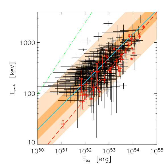
Figure 10: Rest frame peak energy $E_{\rm peak}$ versus isotropic equivalent energy $E_{\rm iso}$. Red filled circles are the 43 GRBs with spectroscopically measured redshifts and published spectral properties (adapted from [55]). The long–dashed line is their best fit (weighting for the errors on both variables) which is reported in Tab. 1. The black crosses are the 442 GRBs with pseudo redshifts derived from the lag–luminosity relation. The solid line is the best fit to these data points which results $E_{\rm peak}\propto E_{\rm iso}^{0.47}$ with a reduced $\chi^{2}_{\rm r}=4.0$ (440 dof). The shaded region represents the 3$\sigma$ scatter of the black points around their best fit line (solid line). The triple–dot–dashed line represents the $E_{\rm peak}-E_{\gamma}$ correlation.

One test that can be performed even without knowing the redshift of GRBs is to check if bursts with measured fluence $S$ and peak energy $E_{\rm peak}^{\rm obs}$ are consistent with the $E_{\rm peak}-E_{\rm iso}$ correlation, by considering all possible redshifts. The application of this test to a sample of BATSE bursts ([103], [104]) led to claim that the $E_{\rm peak}$–$E_{\rm iso}$ correlation is not satisfied by most of the BATSE GRBs without a redshift measurement. Instead, a different conclusion has been reached by [107].

We performed ([108]) a different test by checking if a large sample of GRBs with a pseudo-redshift measurement could indicate the existence of a relation in the $E_{\rm peak}-E_{\rm iso}$ plane, although with a possible larger scatter than that found for the $E_{\rm peak}$-$E_{\rm iso}$ correlation with few GRBs with spectroscopic measured redshifts.

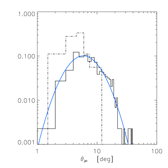
Figure 11: Jet opening angle distributions. The solid histogram represents the $\theta_{\rm jet}$ derived from the large sample of 442 GRBs with pseudo redshifts requiring that they satisfy the $E_{\rm peak}-E_{\gamma}$ correlation ([105],[35] - with the approximation of no scatter). The solid line is the best fit log–normal distribution. The dot-dashed histogram represents the angle distribution of the 19 GRBs with spectroscopic redshifts and well constrained $t_{\rm jet}$.

With a sample of 442 long duration GRBs whose spectral properties has been studied ([109]) and whose redshifts has been derived from the spectral lag–luminosity correlation ([106]), we populated the $E_{\rm peak}-E_{\gamma,\rm iso}$ plane (black crosses in Fig. 10). We found that this large sample of burst produce an $E_{\rm peak}$-$E_{\rm iso}$ correlation (solid line in Fig.10) whose slope (normalization) is slightly flatter (smaller) than that found with the sample of 43 GRBs (red filled circles in Fig.10). The gaussian scatter of the pseudo–redshift bursts around their correlation has a standard deviation $\sigma=0.2$, i.e. consistent with that of the 43 GRBs around their best fit correlation (long-dashed red line in Fig.10). This suggests that indeed a correlation between $E_{\rm peak}$ and $E_{\rm iso}$ exists.

However, it might still be argued that the correlation found with the 43 and with the 442 GRBs have inconsistent normalization, although similar scatter and slopes. This is shown by the 43 GRBs (red filled circles in Fig.10) with spectroscopically measured redshifts which lie on the right tail of the scatter distribution of the 442 GRBs (black crosses) in the $E_{\rm peak}-E_{\rm iso}$ plane. This fact might be interpreted as due to the selection effect of the jet opening angle. In fact, from the scatter of the 442 GRBs we can derive their jet opening angles by assuming that the $E_{\rm peak}$-$E_{\gamma}$ correlation exists and that its scatter is (as shown in [34]) much smaller than that of the $E_{\rm peak}-E_{\rm iso}$ correlation. The $\theta_{\rm jet}$ distribution derived in this way is shown in Fig.11 (solid histogram) and it is well represented by a log-normal distribution (solid line) with a typical $\theta_{\rm jet}\sim 6^{o}$. The $\theta_{\rm jet}$ distribution of the 19 GRBs with measured $t_{\rm jet}$ is also shown (dot-dashed histogram in Fig.11) and it appears shifted to the small–angle tail of the $\theta_{\rm jet}$ distribution of the 442 angles. This suggests that the 43 GRBs, which are used to define the $E_{\rm peak}-E_{\rm iso}$ correlation, have jet opening angles which are systematically smaller than the average value of the distribution and this is what makes them more luminous and, therefore, more easily detected.

Interestingly the fact that the scatter of the 442 GRBs in the $E_{\rm peak}-E_{\rm iso}$ plane around their best fit correlation is gaussian indicates that, if the scatter is due solely to their angle distribution, this is characterized by a preferential angle. If, instead, the angle distribution were flat, we should expect a uniform distribution of the data points around the $E_{\rm peak}-E_{\rm iso}$ correlation.

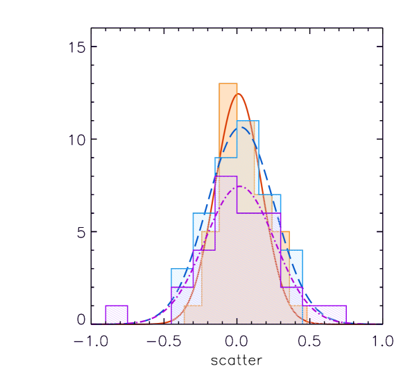
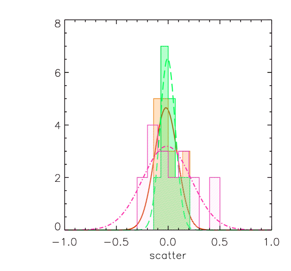
Figure 12: Left: Distribution of the scatter around the correlations involving isotropic quantities (reported in Tab.1). The orange distribution (and solid orange line) represents the scatter distribution (and its gaussian fit) around the $E_{\rm peak}$-$E_{\rm iso}$ correlation. The blue histogram and violet histograms are for the $E_{\rm peak}$-$L_{\rm iso}$ and $V-L_{\rm iso}$ correlation, respectively. Right: Distribution of the scatter around the correlations involving the collimation corrected quantities and of the 3-D empirical correlation (reported in Tab.2). The green distribution (and dashed green line) represents the scatter distribution (and its gaussian fit) around the $E_{\rm peak}$-$E_{\gamma}$ correlation (in the wind circumburst scenario). The orange and pink histograms are for the scatter of the $E_{\rm peak}$-$E_{\gamma}$ (in the homogeneous circumburst medium scenario) and $E_{\rm iso}-E_{\rm peak}-t_{\rm break}$ correlation, respectively.

7 Constraining the cosmological parameters with GRBs

The scatter of the correlations described in the previous sections are compared in Fig.12. The collimation corrected correlations $E_{\rm peak}$–$E_{\gamma,HM}$ and $E_{\rm peak}$–$E_{\gamma,WM}$ or the empirical correlation $E_{\rm peak}$–$E_{\rm iso}$–$t_{\rm break}$, due to their very low scatter can be used to constrain the cosmological parameters. Moreover, all these correlations have an acceptable reduced $\chi^{2}$ in the concordance cosmological model.

As a first test of the possible use of the above correlations for cosmography we show in Fig. 13 the luminosity distance derived with the $E_{\rm peak}$–$E_{\gamma}$ correlation in the HM and WM scenario for the 18 GRBs of the sample discussed in [35]. By comparing the plots with Fig. 3 we note that by using the $E_{\rm peak}$-$E_{\gamma}$ correlation the dispersion of the data points is reduced with respect to the assumption that all GRBs have a unique luminosity (see Sec. 2). Also note that no substantial difference appears if using the $E_{\rm peak}$-$E_{\gamma}$ correlation derived either in the HM or in the WM case (top and lower panel of Fig. 13 respectively).

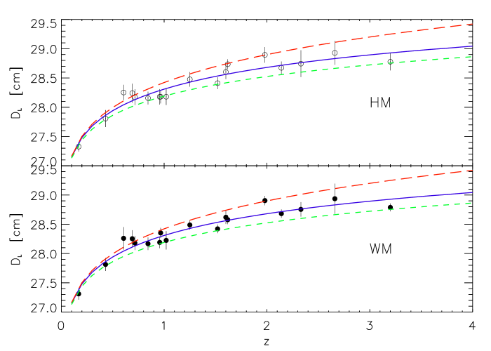
Figure 13: Hubble diagram of the 18 GRBs of the sample of [35] derived with the $E_{\rm peak}$–$E_{\gamma}$ correlations in the HM and WM case. The curves represent different cosmological models: ($\Omega_{M},\Omega_{\Lambda}$)=(0.3,0.7) [solid–blue line], ($\Omega_{M},\Omega_{\Lambda}$)=(0.0,1.0) [long–dashed red line], ($\Omega_{M},\Omega_{\Lambda}$)=(1.0,0.0) [short–dashed green line].

Different methods have been proposed to constrain the cosmological parameters with GRBs ([40], [116], [41]). A common feature of these methods is that they construct a $\chi^{2}$ statistic, based on one of the correlations described before, as a function of two cosmological parameters. The minimum $\chi^{2}$ and the statistical confidence intervals (i.e. 68%, 90% and 99%) represent the constraints on the couple of cosmological parameters.

One important point (see also Sec 7.3) is that the correlations that we have presented so far have been derived assuming a particular cosmological model, i.e. $\Omega_{M}$=0.3, $\Omega_{\Lambda}$=0.7 and $h$=0.7. Indeed, in the $E_{\rm peak}$–$E_{\gamma,HM}$ correlation, for instance, $E_{\rm peak}=E_{\rm peak}^{\rm obs}(1+z)$ is independent from the cosmological model whereas $E_{\gamma}$ depends on the cosmological parameters through the luminosity distance, i.e. $E_{\gamma}=f(4\pi D_{L}^{2}F)/(1+z)$, where $D_{L}$ is a function of ($\Omega_{M}$,$\Omega_{\Lambda}$,$h$) (see Sec.1.1). The need to assume a set of cosmological parameters to compute the above correlations is mainly due to the lack of a set of low redshift GRBs which, being cosmology independent, would calibrate these correlations. Therefore, if we want to fit any set of cosmological parameters with the above correlation we cannot use a unique correlation i.e. obtained in a particular cosmology. This method, which has indeed been adopted by [116], would clearly suffer of such a circular argument.

The “circularity problem” ([117]) can be avoided in two ways: (i) through the calibration of these correlations by several low redshift GRBs (in fact, at $z\leq 0.1$ the luminosity distance has a negligible dependence from any choice of the cosmological parameters $\Omega_{M}$,$\Omega_{\Lambda}$) or (ii) through a solid physical interpretation of these correlation which would fix their slope independently from cosmology. A third possibility, presented in Sec. 7, consists in calibrating the correlations with a set of GRBs with a low dispersion in redshift.

While waiting for a sample of calibrators or for a definitive interpretation, we can search for suitable statistical methods to use these correlations as distance indicators but avoiding the “circularity problem”. The methods that have been used to fit the cosmological parameters through GRBs can be summarized as follows:

• (I) The scatter method ([40]). By fitting the correlation for every choice of the cosmological parameters that we want to constrain (e.g. $\Omega_{M},\Omega_{\Lambda}$) a $\chi^{2}$ surface (as a function of these parameters) is built. The best cosmological model corresponds to the minimum scatter around the correlation (which has to be re-computed in every cosmology in order to avoid the circularity problem) and is identified by the minimum of the $\chi^{2}(\Omega_{M},\Omega_{\Lambda})$ surface.

• (II) The luminosity distance method ([40],[116],[39]). The main steps are: (1) choose a cosmology and fit the $E_{\rm peak}$–$E_{\gamma}$ correlation ; (2) from the best fit correlation the term $E_{\gamma}$ is estimated; (3) from the definition of $E_{\gamma}=f\cdot E_{\rm iso}$ (where also $f=1-\cos\theta_{\rm jet}$ is a function of $E_{\rm iso}$ through $\theta_{\rm jet}$) derive $E_{\rm iso}$ from which (4) the luminosity distance $D_{L,c}$ is computed; (5) build a $\chi^{2}$ by comparing $D_{L,c}$ with that derived from the cosmological model $D_{L}$. By repeating these steps for every choice of the cosmological parameters a $\chi^{2}(\Omega_{M},\Omega_{\Lambda})$ surface is derived. Also in this case the minimum $\chi^{2}$ represents the best cosmology, i.e. the model which best matches the luminosity distance derived from the correlation and that predicted by the model itself.

• (III) The Bayesian method ([41]). The two methods described above are based on the concept that a correlation exists between two variables, e.g. $E_{\rm peak}$ and $E_{\gamma}$. However these correlations are also very likely related to the physics of GRBs and, therefore, they should be unique. This property is not exploited by methods (I) and (II). Firmani et al. ([41]) proposed a more sophisticated method which makes use of both these conditions, i.e. the existence and uniqueness of the correlation. The method is based on the Bayes theorem (e.g. [118]). The basic steps are: (1) choose a cosmology $\bar{\Omega}$ and fit the correlation; (2) test this correlation (i.e. keep it fixed) in all the possible cosmologies $\Omega$ and derive a conditioned probability surface $P(\Omega|\bar{\Omega})$ which represents a “weight” for the starting cosmology $\bar{\Omega}$ (i.e. it describes how all the cosmologies that have been tested “respond” to the starting cosmology); (4) by repeating these steps for different starting cosmologies $\bar{\Omega}$ and combining, at each step, the new conditioned probability with those found in the previous iterations, the Bayesian methods naturally converges to a final probability surface whose maximum represents the best cosmological model.

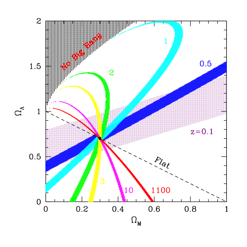
Figure 14: Regions of $\pm$1% variation around lines of constant $d_{\rm L}$ in the ($\Omega_{\rm M}$,$\Omega_{\Lambda}$) plane at redshift 0.5,1,1.5 and 2. assuming that each line passes through the fiducial point($\Omega_{\rm M}$=0.33,$\Omega_{\Lambda}$=0.77).

The last method, which exploits all the information contained in the adopted correlation, has also a practical advantage: it solves the problem of the loitering line which separates Big-Bang and no-Big-Bang universes. As shown in Fig. 14, near this line the luminosity distance stripes are highly wounded–up and clustered. In correspondence to this line in fact $D_{L}$ falls rapidly to zero. If the adopted sample of standard candles extends to very high redshifts, this region can attract the minimum of the $\chi^{2}$ surface, as shown in Fig.1 of [40]. For this reason the Bayesian method is more accurate because it assigns a low probability to the cosmologies near this line (see [41]).

8 Constraints on $\Omega_{M}$ and $\Omega_{\Lambda}$

With the Bayesian method we can constrain the cosmological parameters $\Omega_{M}$ and $\Omega_{\Lambda}$ with the sample of 18 GRBs reported in [35] updated with GRB 051022 (see [44]). In Fig. 15 we show the contours corresponding to the 68%, 90% and 99% confidence levels obtained with all the three correlations, i.e. $E_{\rm peak}$–$E_{\gamma,HM}$ (solid line), $E_{\rm peak}$–$E_{\gamma,WM}$ (dashed line) and the empirical 3D correlation $E_{\rm peak}$–$E_{\rm iso}$–$t_{\rm break}$ (dotted line). We note that the contours obtained with these correlations (of which the first two are model dependent and the third is completely empirical) are consistent one with another. We also note that the centroid of the confidence contours are only slightly different. However, given the large allowance area of the same contours the exact position of the centroid is not relevant, i.e. the contours obtained with GRBs as standard candles are consistent with the concordance model.

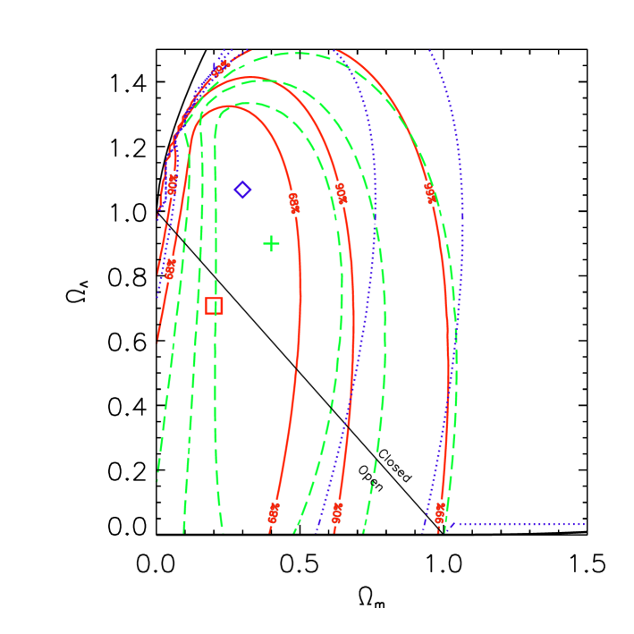
Figure 15: Constraints on the $\Omega_{M}$ and $\Omega_{\Lambda}$ parameters obtained with the Bayesian method through the three correlations: $E_{\rm peak}$–$E_{\gamma,HM}$ (solid red line), $E_{\rm peak}$–$E_{\gamma,WM}$ (dashed green line) and the empirical correlation $E_{\rm peak}$–$E_{\rm iso}$–$t_{\rm break}^{\prime}$ (dotted blue line). The lines correspond to the 68%, 90% and 99% confidence contours.

8.1 Statistical errors

One of the critical issue in the use of the three correlations for cosmology is related to statistical errors. There are, in fact, two major sources of errors which shape the contours obtained with GRBs: the statistical errors associated with the observables used to calculate $E_{\rm peak}$ and $E_{\gamma}$ and the errors on the best fit parameters (slope and normalization) of the correlation resulting from the fitting procedure. These errors enters in the construction of the $\chi^{2}$ surface.

In particular, the issue of accounting for all the sources of errors makes the contours particularly large as in the case of the empirical 3D correlation which involves three observables (with their statistical uncertainties) and three fit parameters (with their errors, resulting from the best fit of the data points). As a simple test we compare in Fig. 16 the constraints on $\Omega_{M}$ and $\Omega_{\Lambda}$ when accounting only for the errors on the observables (solid–red contours) or when accounting also for the errors on the best fit parameters (dashed blue contours). In Fig. 16 (left panel) we show the constraints obtained with the empirical $E_{\rm peak}$–$E_{\rm iso}$–$t_{\rm break}$ correlation by ignoring (solid contours) the errors associated to the the best fit parameters which in this case are the normalization and 2 slopes (because the correlation is expressed, for instance, as $E_{\rm iso}$ as a function of $E_{\rm peak}$ and $t_{\rm break}$). The same figure shows, instead, that if we account for all the errors, we find (dashed blue contours) considerably larger constraints. This difference is also represented in the right panel of Fig. 16 where the error on the distance modulus $\mu$ obtained accounting for all the errors is represented versus the same quantity obtained including only the errors on the observables.

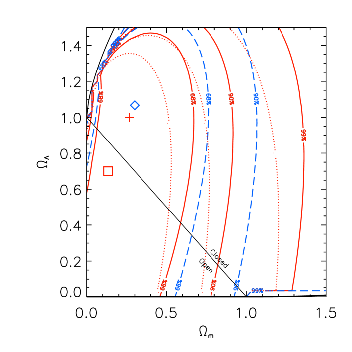
Figure 16: Left:Constraints on the cosmological parameters $\Omega_{M}$,$\Omega_{\Lambda}$ obtained with the empirical 3D correlation and the updated sample of 19 GRBs. The solid (red) contours are obtained by considering, as in [39], only the errors on the variables, i.e. $E_{\rm peak}$, $E_{\rm iso}$ and $t_{\rm break}$. The long–dashed blue contours include also the errors on the best fit parameters. The dotted contours are obtained with the original sample of 14 GRBs used by [39], accounting only for the errors on the variables. Right: Errors on the distance modulus $\mu$ computed considering the errors on the best fit correlation parameters (k,A) versus the same error computed ignoring these uncertainties and considering only the errors on $E_{\rm\gamma,iso}$, $E_{\rm p}$ and $t_{\rm break}$. In this case we assumed that the exponent of $t_{\rm break}$ is linear and we ignored the error on this parameter.

The dotted (red) contours in Fig. 16 (left panel) are obtained with the sample of 14 GRBs reported in the original work of [39] without including the errors on the best fit parameters. Here we adopted the Bayesian method to derive all the cosmological contours. Moreover, another possible reason for the difference between our contours (red dotted in Fig. 16) and the slightly smaller contours reported in [39] might be the fact that our method for fitting the 3D empirical correlation takes into account the errors on the three variables and adopts a the $\chi^{2}$ minimization method to find the best fit parameter values, whereas the multiregression analysis ([39]) does not account for all the errors on the observables.

8.2 Combining GRBs and SNIa

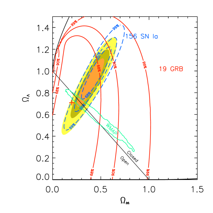
Figure 17: Constraints on the cosmological parameters $\Omega_{\rm M}$, $\Omega_{\Lambda}$ obtained with the updated sample of 19 GRBs, in the homogeneous density case (HM). The solid (red) contours, obtained with the 19 GRBs alone, represent the 68.3%, 90% and 99% confidence regions. The center of these contours (red cross) corresponds to a minimum $\chi^{2}=15.25/17$ dof and has $\Omega_{M}=0.23$ and $\Omega_{\Lambda}=0.81$. The contours obtained with the 156 SN Ia of the “Gold” sample of [11] are shown by the dashed (blue) lines. The joint GRB+SN constraints are represented by the shaded contours. We also show the 90% confidence contours obtained with the WMAP data (from [6]).

One important consequence of using GRBs as standard candles through the $E_{\rm peak}$-$E_{\gamma}$ correlations or the empirical 3-D $E_{\rm iso}$-$E_{\rm peak}$-$t_{\rm break}$ correlation is that they can be combined with SNIa. With respect to SNIa, GRBs already extend in a redshift range which is beyond the present (and future) SNIa redshift limit (i.e. $z\sim 1.7$ predicted for SNAP - e.g. [119]). Furthermore, GRBs are detected in the $\gamma$ ray band which is unaffected by dust extinction limitations. However, SNIa are detected in large number also at very low redshifts and their “stretching–luminosity” correlation can be well calibrated. Therefore, GRBs should be considered as complementary to SNIa at very high redshisfts.

In Fig. 17 we show the contours obtained with GRBs (in the HM case) and we combine them with the constraints obtained for a large sample of 156 SNIa (the “gold” sample of [11]). The combined fit is clearly dominated by the large number of SNIa with respect to GRBs (a factor 10 more numerous), however, the power of GRBs is to make the joint contours more consistent with the concordance model, also due to the different orientation of the contours obtained by these two probes (see Sec. 1).

8.3 Cosmological constraints with the $L_{\rm iso}$-$E_{\rm peak}$-$T_{0.45}$ correlation

Finally, we present in Fig. 19 the constraints ([37]) on the parameters $\Omega_{\rm M}$ and $\Omega_{\Lambda}$ obtained with the “prompt–emission” correlation $L_{\rm iso}$-$E_{\rm peak}$-$T_{0.45}$ (see Sec. 3.5).

First we can apply the scatter method (I) to test if this correlation is, indeed, sensitive to the cosmological parameters. We indeed show in Fig. 18 smallest scatter is obtained for ($\Omega_{\rm M}$,$\Omega_{\Lambda}$)=(0.3,0.7), i.e. very close to the concordance model.

Figure 18: Contours at 68.3%, 95.5%, and 99.7% CL’s obtained from projecting to the $\Omega_{\rm M}$, $\Omega_{\Lambda}$ plane the $L_{\rm iso}$-$E_{\rm peak}$-$T_{0.45}$ relation that is obtained from the fit of the GRB data at each value of the ($\Omega_{\rm M}$,$\Omega_{\Lambda}$) pair. This plot shows that the $L_{\rm iso}$-$E_{\rm peak}$-$T_{0.45}$ relation is sensitive to cosmology, so that it may be used to discriminate cosmological parameters if an optimal method to circumvent the circularity problem is used. The diagonal line corresponds to the flat geometry cosmology, the upper curve is the loitering limit between Big Bang and no Big Bang models, and the lower curve indicates the division between accelerating and non-accelerating universes.

By adopting the same Bayesian method described above, we note that the constraints obtained with this new correlation with a sample of only 19 GRBs are tighter than those obtained with the $E_{\rm peak}$-$E_{\gamma}$ correlation (Fig. 17).

Figure 19: Constraints on the ($\Omega_{\rm M}$,$\Omega_{\Lambda}$) plane for a $\Lambda$ cosmology from the GRB Hubble diagram using our Bayesian method to circumvent the circularity problem and from the gold set of SNIa of [11] (thin solid lines). The GRB constraints are obtained with the $L_{\rm iso}$-$E_{\rm peak}$-$T_{0.45}$ correlation.

The best cosmological model, indicated by the star symbol in Fig. 19, corresponds to $\Omega_{\rm M}=0.31^{+0.09}_{-0.08}$,$\Omega_{\Lambda}=0.80^{+0.20}_{-0.30}$ (1$\sigma$ uncertainty), i.e. vary close to the flat geometry case. Indeed, if a flat geometry is assumed, we find $\Omega_{\rm M}=0.29^{+0.08}_{-0.06}$ ([37]).

9 The future of GRB-cosmology

The luminosity distance test requires large samples of sources possibly distributed over a wide redshift range. This can be understood from Fig. 14 which shows the topology of the luminosity distance as a function of the cosmological parameters that we want to constrain. In this case we consider $\Omega_{M}$ and $\Omega_{\Lambda}$ as the two free parameters. The stripes in Fig. 14 show the degeneracy of the $\Omega_{M}$ and $\Omega_{\Lambda}$ parameters and how this degeneracy varies with the redshift $z$. Each stripe represents, for a fixed redshift $z$, all the possible combinations ($\Omega_{M}$,$\Omega_{\Lambda}$) which give a luminosity distance equal within 10%. By increasing the redshift the stripes wound up due to the topology of the luminosity distance as a function of these two parameters, i.e. ($\Omega_{M}$,$\Omega_{\Lambda}$) (see [117]). It is clear from Fig. 14 that if we use a sample of sources distributed over a wide range of redshifts we “intersects” differently oriented stripes and we end up with accurate constraints on the two cosmological parameters. On the other hand a sample of sources distributed in a very small redshift range would not break the degeneracy of these two parameters. The requirement of a large number of sources instead is a key ingredient to reduce the possible effect of systematic errors.

The present open issues related to the use of GRBs in cosmologies are: (1) the low number of events: the sample of GRBs which can be used to constrain the cosmological parameters through the above correlations are in fact 19 (to date); (2) the lack of a calibration sample, i.e. the absence of GRBs at very low redshifts in the sample used for cosmology, does not allow to calibrate the correlation and requires to adopt a method to fit the cosmological parameters which avoids the circularity problem; (3) the possible lensing effects which might introduce a dispersion of the luminosities and energetics of GRBs at very high redshifts. The latter point, however, if present, could be easily recognized: if strong lensing by compact objects (if by clusters they should be observed) is present, we should observe a repetition of a similar structure (e.g. peak shape) within the same light curve. Moreover, the lack of a theoretical interpretation of the physical nature of all these correlations represents a still open issue.

The increase of the number of bursts which can be used to measure the cosmological parameters, and the possible calibration of the correlations would greatly improve the constraints that are presently obtained with few events and with a non–calibrated correlation.

In order to use GRBs as a cosmological tools, through the above correlations, three fundamental parameters, i.e. $E_{\rm peak}$, $E_{\gamma}$ and $t_{\rm jet}$, should be accurately measured. This requirement also applies to the case of the empirical correlation of [39]. On the other hand the $L_{\rm iso}$-$E_{\rm peak}$-$T_{0.45}$ does not require the knowledge of the afterglow emission because it completely relies on the prompt emission observables.

However, only a limited number of GRBs, i.e. 19 out of $\sim$ 70 with measured $z$, can be used as standard candles. Presently the most critical observable is the peak energy $E_{\rm peak}$. In fact, the limited energy range (15–150 keV) of BAT on board Swift allows to constrain with only moderate accuracy the $E_{\rm peak}$ of particularly bright–soft bursts. However, given the perspective of the cosmological investigation through GRBs, it is worth exploring the power of using GRBs as cosmological probes. The other still open issue related to the use of GRBs as standard candles is the so called “circularity problem” (see Sec. 5).

To the aim of calibrating this spectral–energy correlation, GRBs at low redshift are required. In fact for $z<0.1$ the difference in the luminosity distance computed for different choices of the cosmological models [for $\Omega_{\rm M},\Omega_{\Lambda}\in(0,1)$] is less than 8%. However, if (long) GRBs are produced by the death of massive stars, they are expected to roughly follow the cosmic star formation history (SFR) and we should expect that the rate of low redshift events is quite small at $z<0.1$. Indeed, a considerable number of GRBs with $z>1$ should be collected in the next years by presently flying instruments (Swift and Hete–II). At such large redshifts, the cosmological models starts to play an important role. However, if it will be possible to have a sufficient number of GRBs with a similar redshift, it might still be possible to calibrate the slope of these correlations also with high redshift GRBs (see Sec. 7.3).

9.1 The simulation

In order to fully appreciate the potential use of GRBs for the cosmological investigation, we simulate a sample of bursts comparable in number to the “Gold” sample of 156 SN Ia. Similar simulations have been presented before (e.g. [42],[39]). However, different assumptions can be made on the properties of the simulated sample and the results are clearly dependent on these assumptions. In particular, simulations based on the observed parameters ([42]) strongly depend on the almost unknown selection effects which shape the observed distributions.

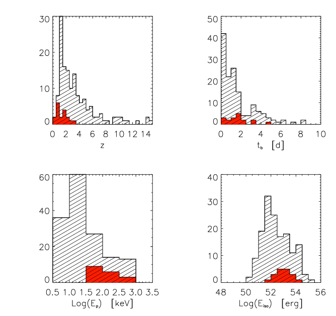
Figure 20: Distributions of redshift $z$, jet break time $t_{b}$, observed peak energy $E_{\rm peak}^{\rm obs}$ and isotropic equivalent energy $E_{\rm iso}$ for the 150 simulated bursts (hatched histograms). Also show (solid filled histogram) are the distributions of the sample of 19 GRBs used to derive the $E_{\rm peak}-E_{\rm iso}$ correlation.

We adopt here a method which makes use of the intrinsic properties of GRBs as described by the $E_{\rm peak}$-$E_{\gamma}$ and the $E_{\rm peak}$-$E_{\rm iso}$ correlations. We use the most updated version of these correlations as found with the sample of 19 GRBs described in the previous sections.

The assumptions of our simulation are:

• we assume that GRBs have an “isotropic energy” function which is described by a powerlaw $N(E_{\rm iso})\propto E_{\rm iso}^{\delta}$ for $E_{\rm iso,min}<E_{\rm iso}<E_{\rm iso,max}$ (e.g. [38]). Further we assume that GRBs follow the cosmic star formation rate (SFR - as modeled in [120] );

• we use the $E_{\rm peak}$-$E_{\rm iso}$ correlation to derive the peak energy $E_{\rm peak}$ and we model the scatter of the simulated GRBs around the $E_{\rm peak}$-$E_{\rm iso}$ correlation with a gaussian distribution with $\sigma=0.2$ (which corresponds to the present scatter of the 19 GRBs around their best fit correlation);

• we use the $E_{\rm peak}$-$E_{\gamma}$ correlation as found with the 19 GRBs in the WM case to calculate $E_{\gamma}$ and we model the scatter of the simulated GRBs around the $E_{\rm peak}$-$E_{\gamma}$ correlation with a gaussian distribution with $\sigma=0.08$ (as found in Sec. 4);

• we derive the jet opening angle $\theta_{\rm j}$ and the corresponding jet break time $t_{\rm break}$;

• we assume that the simulated GRB spectra are described by a Band model spectrum ([121]) with typical low and high energy spectral photon indices $\alpha=-1.0$ and $\beta=-2.5$ and require that the simulated GRB fluence in the 2-400 keV energy band is above a typical instrumental detection threshold $S\sim 10^{-7}$ erg/cm². This corresponds roughly to the present threshold of Hete-II in the same energy band.

Following the procedure described above we built a sample of 150 GRBs with the relevant parameters: $z$, $E_{\rm iso}$, $E_{\rm peak}$, $t_{\rm break}$. The errors associated to these parameters are assumed to be cosmology invariant and they are set to 10%, 20% and 20% for $E_{\rm iso}$, $E_{\rm peak}$, $t_{\rm break}$ respectively. Moreover, we model the GRB intrinsic isotropic energy function with a powerlaw with $\delta=-1.3$ between two limiting energies ($10^{49}$-$10^{55}$ erg). This particular choice of parameters is due to the requirement that the distributions of the relevant quantities (shown in Fig. 20) of the simulated sample are consistent with the same distributions for the present sample of 19 GRBs (red histograms in Fig. 20). The sample is simulated in the standard cosmology ($\Omega_{M}=0.3$ and $\Omega_{\Lambda}=h=0.7$). We compare the distributions of $z,t_{b},E_{p}eak$ and $E_{iso}$ for the 150 simulated bursts with the same distributions of the 19 GRBs in Fig. 20. We note that by choosing a steeper energy function we obtain a much larger number of XRF and XRR with respect to normal GRBs.

9.2 Cosmological constraints with the simulated sample

The results obtained with the sample of 150 simulated GRBs are presented in Fig. 21: in this case the constraints are comparable with those obtained with SNIa. By comparing the 1$\sigma$ contours of GRB alone from Fig.21 to the same contours (solid line) of Fig. 17 (obtained with the 19 GRBs), we note an improvement (of roughly a factor 10) with the sample of 150 bursts.

Fig. 21 also shows the different orientation of the GRB contours with respect to SN Ia due to the “topology” of the luminosity distance as a function of the $\Omega_{M}$-$\Omega_{\Lambda}$ parameters. Most GRBs of our simulated sample are, in fact, at $z\sim 2$, and this explains the tilt of the contours in the $\Omega$ plane. Clearly the contours obtained through the simulated sample depends on the assumptions: in particular we have no knowledge of the burst intrinsic energy function $N(E_{\rm iso})$. However, if we accept the hypothesis to model it with a simple powerlaw, we can change the slope and also include the possible effect of the redshift evolution. We tested the dependence from these assumptions of the constraints reported in Fig. 21 and found that, by assuming different $\delta$ values and a $(1+z)$ evolutionary factor, what changes is the redshift distribution of the simulated sample and therefore the orientation of the GRB contours in Fig. 21. The same happens if we adopt, for the same choice of parameters reported above, a different SFR.

Further, we can also use the CMB priors. First we assume the cosmological constant model with the 2 CMB priors, i.e (i) $\Omega_{tot}=1$ and (ii) $\Omega_{M}=0.14/h^{2}$. In this case the only free parameter is $h$ (or equivalently $\Omega_{M}$).We obtain the best fit values of $\Omega_{M}=0.27\pm 0.02$ and $\Omega_{\Lambda}=0.73\pm 0.02$.

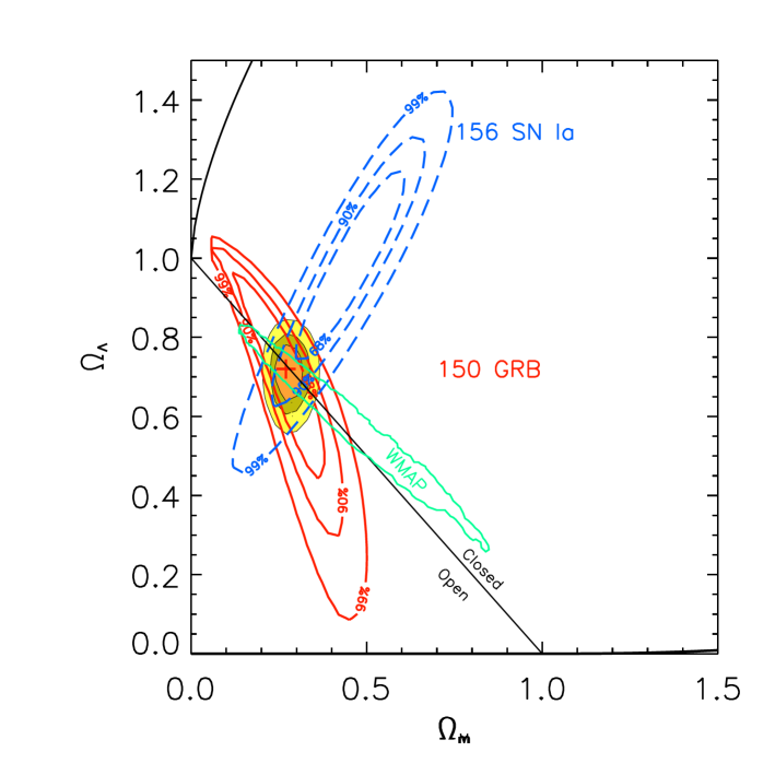
Figure 21: Wind density profile case. Constraints on the cosmological parameters $\Omega_{\rm M}$,$\Omega_{\Lambda}$ obtained with the sample of 150 GRBs simulated by assuming the $E_{\rm peak}$-$E_{\gamma}$ correlations derived in the wind density profile. The solid (red) contours, obtained with the 19 GRBs alone, represent the 68.3%, 90% and 99% confidence regions on the pair of cosmological parameters. The contours obtained with the 156 SN Ia of the “Gold” sample of [11] are shown by the dashed (blue) lines. The joint GRB+SN constraints are represented by the shaded contours.

One of the major promises of the cosmological use of GRBs is related to the possibility to study the nature of Dark Energy with such a class of “standard candles” extending out to very large redshifts. With the present sample of 19 GRBs we can explore the equation of state (EOS) of DE, which can be parametrized in different ways. Given the already considerably large dispersion of GRB redshifts (i.e. between 0.168 to 3.2 for the 19 GRBs of our sample) we adopt the parametrization proposed by [122] for the EOS of DE, i.e. $P=w(z)\rho$, where:

$$w(z)=w_{0}+{w_{a}z\over 1+z}$$ (1)

With this assumption the luminosity distance, as derived from the Friedman equations, is

$$d_{L}(z;\Omega_{M},w_{0},w_{a})={c(1+z)\over H_{0}}\int_{0}^{z}dz[\Omega_{M}(1+z)^{3}$$

$$\,\,\,\,\,\,\,\,\,\,\,\,\,\,\,\,+(1-\Omega_{\rm M})(1+z)^{3+3w_{0}+3w_{a}}\exp\left(-3w_{a}{z\over 1+z}\right)]^{-1/2}$$ (2)

which depends on the ($w_{0}$,$w_{a}$) parameters. Note that Eq. 2 is derived with the prior of a flat Universe.

First, we can assume the CMB prior of a flat universe together with the assumption of a non–evolving equation of state of the Dark Energy (i.e. $w_{a}=0$). We show in Fig. 5 the contours obtained with the sample of 150 simulated GRBs and compare with the same constraints derived with the 156 SN Ia of the “Gold” sample. The constraints on $w_{a},w_{0}$ are reported in Fig. 6, assuming $\Omega_{\rm M}=0.3$.

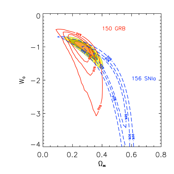
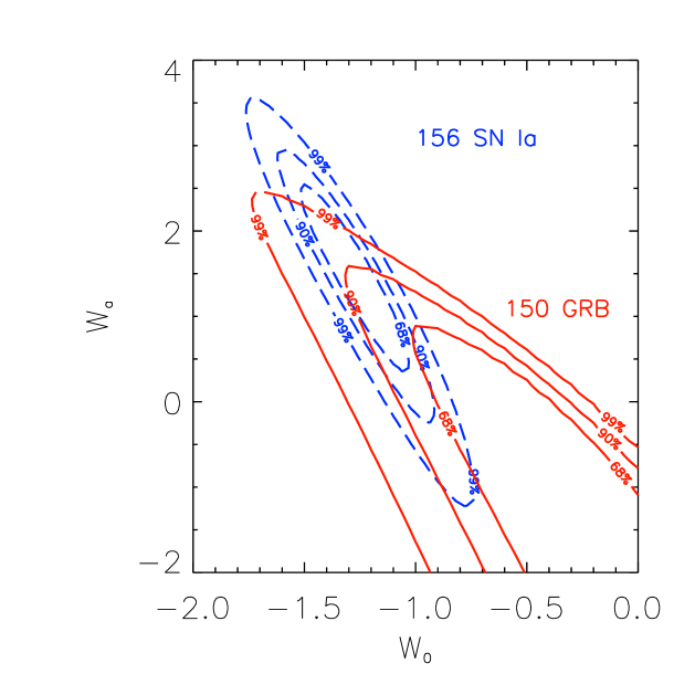
Figure 22: Left: Constraints on the cosmological parameters $w_{0}$, $w_{a}$ obtained with the 150 simulated GRBs (red contours) compared with the same contours obtained with the 156 SNIa of the “Gold” sample. A flat universe is assumed ($\Omega_{\rm tot}=1$). Right: Constraints on the cosmological parameters $w_{0}$, $\Omega_{\rm M}$ obtained with the 150 simulated GRBs (red contours) compared with the same contours obtained with the 156 SNIa of the “Gold” sample. A flat universe is assumed ($\Omega_{\rm tot}=1$).

9.3 The calibration of the correlations

The cosmological use of the $E_{\rm peak}=K\cdot E_{\gamma}^{g}$ correlation suffers from the so called “circularity problem” : this means that both the slope $g$ and the normalization $K$ of the correlation are cosmology dependent.

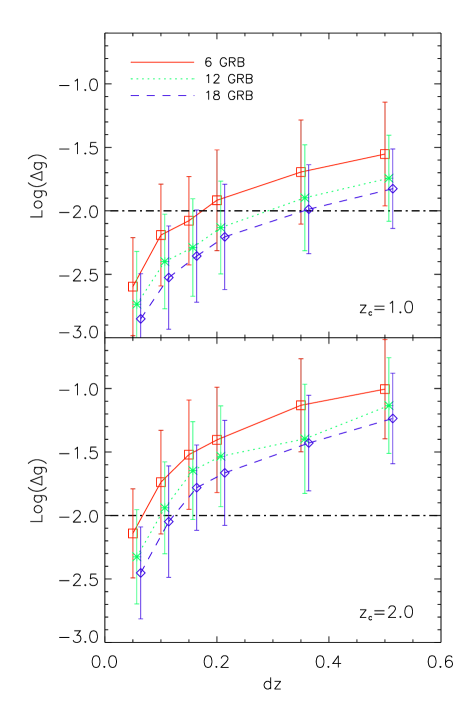
Figure 23: Calibration of the $E_{\rm peak}$-$E_{\gamma}^{g}$ correlation. For different samples of GRBs (6, 12, 18 - corresponding to the solid, dotted and dashed lines respectively) we show the maximum variation $\Delta g$ of the slope of the correlation for any cosmology $\Omega\in(0,1.5)$ as a function of the redshift dispersion of the GRBs $dz$. The dot dashed line represents the limit of variation of 1% of the slope of the correlation. Data points have been shifted along the abscissa for graphical purposes.

In principle this issue could be solved (a) by a large sample of calibrators, i.e. low redshift GRBs for which the luminosity distance $D_{L}$ is practically independent from the cosmological parameters, or (b) by a convincing theoretical interpretation of the physical nature of this correlation. In both cases the slope of the correlation would be fixed.

Case (a) could be realized with 5–6 GRBs at $z<0.1$. However, if (long) GRBs are produced by the core–collapse of massive stars, their rate is mainly regulated by the cosmic SFR and, therefore, the probability of detecting events at $z<0.1$ is small ($\sim 2\times 10^{-5}$). This number should be convolved with the GRB luminosity function: with the assumptions of our simulation we estimate that $\sim 1.3$% of the 150 GRBs should be at low redshifts (i.e. $z<0.4$). Instead, we should expect to have more chances to detect a considerable number (up to $\sim 31$%) of intermediate redshift GRBs ($z\sim 1-2$) where the cosmic SFR peaks.

For this reason we explore the possibility to calibrate the correlation using a sufficient number of GRBs within a small redshift bin centered around any redshift. In fact, if we could have a sample of GRBs all at the same redshift the slope of the $E_{\rm peak}$-$E_{\gamma}$ correlation would be cosmology independent. Our objective is, therefore, to estimate the minimum number of GRBs ($N$) within a redshift bin ($dz$) centered around a certain redshift ($z_{c}$) which are required to calibrate the correlation.

In practice the method consists in fitting the correlation for every choice of $\Omega$ using a set of $N$ GRBs distributed in the interval $dz$ (centered around $z_{c}$). We consider the correlation to be calibrated (i.e. its slope to be cosmology independent) if the change of the slope $g$ is less than 1%.

The free parameters of this test are the number of GRBs $N$, the “redshift slice” $dz$ and the central value of the redshift distribution $z_{c}$. By Monte Carlo technique we use the sample simulated in Sec. 7.1 under the WM assumption to minimize the variation of $\Delta g(\Omega;N,dz,z_{c})$ over the $\Omega_{M},\Omega_{\Lambda}\in(0,1.5)$ plane as a function of the free parameters $(N,dz,z_{c})$.

We tested different values of $z_{c}$ and different redshift dispersions $dz\in(0.05,0.5)$. We required a minimum number of 6 GRBs to fit the correlation in order to have at least 4 degrees of freedom. We report our results in Fig. 23. We show the variation of $\Delta g$ as a function of $dz$ for different samples (6, 12, 18 GRBs - solid, dotted and dashed curves in Fig. 23). The error bars show the width of the distribution of the simulation results and not the uncertainty on the average value. At any redshift the fewer the number $N$ of GRBs the larger the change of $\Delta g$ (for the same $dz$) because the correlation is less constrained. The dependence from $z_{c}$ is instead different: for larger $z_{c}$ we require a smaller bin $dz$ to keep $\Delta g$ small.

From the curves reported in Fig. 23 we can conclude that already 12 GRBs with $z\in(0.9,1.1)$ might be used to calibrate the slope of the $E_{\rm peak}$-$E_{\gamma}$ correlation. At redshift $z_{c}=2$ instead we require a smaller redshift bin i.e. $z\in(1.95,1.05)$. We find that $N=12$ GRBs with $z\in(0.45,0.75)$ can be used to achieve the same 1% precision in the calibration. However, one key ingredient is that the GRBs used to calibrate the correlation do not have the same peak energy otherwise they would collapse in one point in the $E_{\rm peak}$-$E_{\gamma}$ plane. Within the present sample of 19 GRBs there are only 4 GRBs within the redshift interval 0.4–0.8 (i.e. 050525, 041006, 020405 and 051022) and 2 of these (050525 and 041006) have a very similar $E_{\rm peak}$.

We conclude stressing that the three correlations that can be used to constrain the cosmological parameters, i.e. the $E_{\rm peak}$-$E_{\gamma}$ (either in the HM and WM case - [34, 40, 41, 35, 44]), the empirical $E_{\rm iso}$–$E_{\rm peak}$–$t_{\rm break}$ correlation ([39]) and the $L_{\rm iso}$-$E_{\rm peak}$-$T_{0.45}$ correlation ([36, 37]), all involve the peak energy $E_{\rm peak}$ of the GRB prompt emission spectrum. This observable can be properly measured with a detector operating over a wide energy range extending up to few MeV as it could be conceived by future missions dedicated to collect and study the prompt and afterglow properties of GRB to be used as standard candles for cosmology ([43]).

10 Acknowledgements

We would like to thank F. Tavecchio, D. Lazzati, L. Nava and M. Nardini for stimulating discussions. We are deeply grateful to Annalisa Celotti for years of fruitful and enjoying collaboration. The bibliography is clearly incomplete and we apologize for any minor or major missing reference.

References

References

- [1] Liddle 2004, MNRAS, 351, L49
- [2] Lahav & Liddle 2006, Preprint, astro-ph/0601168
- [3] Sanders 2004, Preprint, astro-ph/0402065
- [4] Elizalde 2004, Preprint, astro-ph/0409076
- [5] Kunz, Trotta & Parkinson 2006, Preprint, astro-ph/0602378
- [6] Spregel et al. 2003, ApJS, 148, 175
- [7] Spregel et al. 2006, Preprint, astro-ph/0603449
- [8] http://www.mpe.mpg.de/j̃cg/grbgen.html
- [9] Knop et al., 2003, ApJ, 598, 102
- [10] Torny 2003, ApJ, 594, 1
- [11] Riess et al. 2004, ApJ, 607, 665
- [12] Astier et al., 2006, A&A, 447, 31
- [13] Riess et al. 1998, AJ, 116, 1009
- [14] Perlmutter et al. 1999, ApJ, 517, 565
- [15] Riess et al. 2000, ApJ, 536, 62
- [16] Filippenko 2004, Preprint, astro-ph/0410609
- [17] Cole et al. 2005, MNRAS, 362, 505
- [18] Eisenstein et al. 2005, ApJ, 633, 560
- [19] Hu, Eisenstein & Tegmark, 1998, PhR, 80, L5255
- [20] White et al., 1993, Nature, 366, 429
- [21] Refregier 2003, ARA&A, 41, 645
- [22] Kawai et al. 2005, CGN, 3937
- [23] Fiore et al., 2000, ApJ, 544, L7
- [24] Lamb 2002, Preprint, astro-ph/0210434
- [25] Lamb & Haiman 2003, Preprint, astro-ph/0312502
- [26] Stratta et al. 2005, A&A, 441, 83
- [27] Chen et al. 2005, ApJ, 634, L25
- [28] Fiore et al., 2005, ApJ, 624, 853
- [29] Berger et al. 2005, Preprint, astro-ph/0511498
- [30] Lazzati 2005, Preprint, astro-ph/0505044
- [31] Bromm & Loeb, 2006, ApJ in press, astro-ph/0509303
- [32] Inoue et al. 2004, ApJ, 601, 644
- [33] Murakami et al. 2005, ApJ, 625, L13
- [34] Ghirlanda, Ghisellini & Lazzati 2004, ApJ, 616, 331
- [35] Nava et al. 2006, A&A, 450, 471
- [36] Firmani et al. 2006, MNRAS, in press, astro-ph/0605073
- [37] Firmani et al. 2006, MNRAS, submitted, astro-ph/0605267
- [38] Firmani et al., 2004, ApJ, 611, 1033
- [39] Liang & Zhang 2005, ApJ, 633, 611
- [40] Ghirlanda et al. 2004, ApJ, 613,L13
- [41] Firmani et al. 2005, MNRAS, 360, L1
- [42] Xu, Dai & Liang 2005, ApJ, 633, 603
- [43] Lamb et al. 2005,Preprint, astro-ph/0507362
- [44] Ghirlanda et al. 2006, A&A in press, astro-ph/0511559
- [45] Perlmutter & Schmidt 2003, Preprint,astro-ph/0303428
- [46] Phillips 1993, ApJ, 413, L105
- [47] Riess, Press & Kirshner, 1995, ApJ, 438, L17
- [48] Hamuy et al. 1996, AJ, 112, 2398
- [49] Goldhaber et al. 2001, ApJ, 558, 359
- [50] Riess, Press & Kirshner, 1996, ApJ, 473, 88
- [51] Gherels N. et al., 2004, ApJ, 611, 1005
- [52] Berger et al. 2005, ApJ, 634, 501
- [53] Sakamoto et al. 2005, ApJ, 629, 311
- [54] Paciesas et al. 1999, ApJS, 122, 465
- [55] Amati 2006, A&A submitted, astro-ph/0601553
- [56] Ghirlanda et al. 2005, MNRAS, 360, L45
- [57] Preece R. et al., 2000, ApJS, 126, 19
- [58] Frail, Kulkarni & Sari, 2001, ApJ, 562, L55
- [59] Bloom, Frail & Kulkarni, 2003, ApJ, 594, 674
- [60] Waxman, Kulkarni & Frail, 1998, ApJ, 497, 288
- [61] Fruchter et al. 1999, ApJ, 519, L13
- [62] Rohads et al. 1997, ApJ, 487, L1
- [63] Sari, Piran & Haplern, ApJ, 519, L17
- [64] Dar 1999, A&AS, 138, 505
- [65] Norris et al. 1996, ApJ, 459, 393
- [66] Norris, 2002, ApJ, 579, 386
- [67] Li et al., 2005, ApJ, 619, 983
- [68] Ford et al. 1995,ApJ, 439, 307
- [69] Kocevsky & Edison 2003, ApJ, 594, 385
- [70] Bobbing & Fenimore 2000, ApJ, 535, L29;
- [71] Ryde 2005, A&A, 429, 869
- [72] Feng, Li–Ming & Zhuo, 2005, MNRAS, 362, 59
- [73] Norris, Marani & Bonnel 2000, ApJ, 534, 248
- [74] Schaefer 2004, ApJ, 602, 306
- [75] Daigne & Mochkovitch, 2003,MNRAS, 342, 587
- [76] Crider et al. 1999, ApJ, 519, 206
- [77] Liang & Kargatis, 1996, Nature, 381, 495
- [78] Salmonson, 2000, ApJ, 544, 115
- [79] Ioka & Nakamura 2001, ApJ, 554, L163
- [80] Band, Norris & Bonnell 2004 ApJ, 613, 484
- [81] Lamb, Graziani & Smith 1993, ApJ, 413, L11
- [82] Walker, Schaefer & Fenimore, 2000, ApJ, 537, 264
- [83] Bersier et al. 2003, ApJ, 584, L43
- [84] Sato et al. 2003, ApJ, 599, L9
- [85] Sari & Piran 1997, ApJ, 485, 270
- [86] Kobayashi, Piran & Sari 1997, ApJ, 490, 92
- [87] Dermer & Mitman, 1999, ApJ, 513, L5
- [88] Fenimore & Ramirez–Ruiz, 2000, Preprint, astro–ph/0004176
- [89] Reichart et al. 2001, ApJ, 552, 57
- [90] Guidorzi et al. 2005, MNRAS, 363, 315
- [91] Guidorzi et al. 2005, MNRAS, 364, 163
- [92] Xin & Paczynski, 2006, MNRAS, 366, 219
- [93] Reichart et al. 2005, ApJ , astro-ph/0508111
- [94] DÁgostini 2005, Preprint, physics/0511182
- [95] Lloyd & Ramirez–Ruiz 2002 ApJ, 576, 101
- [96] Amati et al. 2002, A&A, 390, 81
- [97] Lamb, Donaghy & Graziani 2004 NewAR, 48, 459
- [98] Eichler & Lenvinson 2004, ApJ, 614, L13
- [99] Levinson & Eichler, 2005, ApJ, 629, L13
- [100] Yamazaki, Yoka & Nakamura 2004, ApJ, 606, L33
- [101] Toma, Yamazaki & Nakamura 2005, ApJ, 635, 481
- [102] Rees & Meszaros 2005, ApJ, 628, 847
- [103] Nakar & Piran 2005, MNRAS, 360, L73
- [104] Band & Preece 2005, ApJ, 627, 319
- [105] Ghirlanda et al., 2005, Il nuovo Cimento, 28, 303
- [106] Band D., Norris & Bonnel, 2004, ApJ, 613, 484
- [107] Bosnjak et al. 2005, MNRAS, in press, astro-ph/0502185
- [108] Ghirlanda, Ghisellini & Firmani, 2005, MNRAS, 361, L10
- [109] Yonetoku et al. 2004, ApJ, 609, 935
- [110] Schaefer 2003, ApJ, 583, L67
- [111] Chevalier & Li 2000, ApJ, 536, 195
- [112] Ramirez–Ruiz, 2005, ApJ, 625, L91
- [113] Watson et al. 2005, ApJ, 636, 967
- [114] Cobb et al. 2006, Preprint, in press, astro-ph/0603832
- [115] Ghisellini G., et al., 2006, Preprint, astro-ph/0605431
- [116] Dai, Liang & Xu, 2004, ApJ, 612, L101
- [117] Ghisellini et al. 2005, Il nuovo Cimento, 28, 639
- [118] Wall & Jenkins 2003, Practical Statistics for Astronomers, Cambridge University Press.
- [119] Aldering et al. 2002 Proc. SPIE, 4835, 146
- [120] Porciani & Madau 2001, ApJ, 548, 522
- [121] Band et al. 1993, ApJ, 413, 281
- [122] Linder & Huterer 2005, Phys. Rev. D, 72, 043509